Article

Post-Heuristic Cancer Segmentation Refinement over MRI Images and Deep Learning Models

by
Panagiotis Christakakis
and
Eftychios Protopapadakis
*
Department of Applied Informatics, University of Macedonia, Egnatia 156, 546 36 Thessaloniki, Greece
*
Author to whom correspondence should be addressed.
AI 2025, 6(9), 212; https://doi.org/10.3390/ai6090212
Submission received: 31 July 2025 / Revised: 27 August 2025 / Accepted: 29 August 2025 / Published: 2 September 2025

Abstract

Lately, deep learning methods have greatly improved the accuracy of brain-tumor segmentation, yet slice-wise inconsistencies still limit reliable use in clinical practice. While volume-aware 3D convolutional networks achieve high accuracy, their memory footprint and inference time may limit clinical adoption. This study proposes a resource-conscious pipeline for lower-grade-glioma delineation in axial FLAIR MRI that combines a 2D Attention U-Net with a guided post-processing refinement step. Two segmentation backbones, a vanilla U-Net and an Attention U-Net, are trained on 110 TCGA-LGG axial FLAIR patient volumes under various loss functions and activation functions. The Attention U-Net, optimized with Dice loss, delivers the strongest baseline, achieving a mean Intersection-over-Union (mIoU) of 0.857. To mitigate slice-wise inconsistencies inherent to 2D models, a White-Area Overlap (WAO) voting mechanism quantifies the tumor footprint shared by neighboring slices. The WAO curve is smoothed with a Gaussian filter to locate its peak, after which a percentile-based heuristic selectively relabels the most ambiguous softmax pixels. Cohort-level analysis shows that removing merely 0.1–0.3% of ambiguous low-confidence pixels lifts the post-processing mIoU above the baseline while improving segmentation for two-thirds of patients. The proposed refinement strategy holds great potential for further improvement, offering a practical route for integrating deep learning segmentation into routine clinical workflows with minimal computational overhead.

1. Introduction

Lower-grade gliomas (LGGs) are diffuse primary brain tumors classified by the World Health Organization (WHO) as grade II or III. They typically grow more slowly than grade IV glioblastomas, yet still pose serious clinical challenges due to their invasive nature [1]. Patients with LGG often suffer seizures, neurological deficits, and cognitive impairment [2,3]. Magnetic Resonance Imaging (MRI) is the modality of choice for brain tumor evaluation, providing detailed soft-tissue contrast needed to visualize tumor extent. Accurate MRI-based segmentation of LGGs can quantify tumor size, shape, and location, information essential for treatment planning and assessing response [1]. However, manual segmentation by experts is labor-intensive and prone to inter-observer variability, motivating the need for automated, reliable tumor segmentation methods [4].
Automating LGG segmentation is challenging due to the tumors’ variability and imaging appearance [4]. These tumors exhibit irregular, diffuse morphologies with heterogeneous sub-regions, often lacking well-defined borders, making boundary detection difficult. Even expert raters can disagree on ambiguous regions when MRI intensity gradients are smooth [5,6]. Furthermore, obtaining large annotated datasets for training Artificial Intelligent (AI) models is difficult in medical imaging, leading to limited data that can hinder generalization.
Thus, robust segmentation algorithms must handle diverse tumor presentations and scarce training examples. In recent years, Deep Learning (DL), particularly Convolutional Neural Networks (CNNs), has emerged as a transformative tool with numerous applications, especially in the medical domain, enabling models to learn complex features directly from medical imaging data [7,8]. Its ability to analyze complex medical data has demonstrated great potential for improving diagnostic accuracy and prognostic assessments in healthcare [9,10,11]. This extensive capability has advanced medical image analysis, enabling more accurate and efficient identification of various diseases, including different types of tumor segmentation where modern algorithms achieve accuracy approaching inter-rater performance.
However, the deployment of DL models in medical imaging is not without challenges [12,13,14]. Brain MRI is inherently volumetric, comprised of many contiguous slices per patient, very often motivating the use of 3D CNNs instead of classical 2D slice-wise models [15,16]. Unlike 2D networks that analyze slices independently, 3D CNNs leverage inter-slice context for more coherent segmentations at the cost of significantly higher memory and computation demands (often necessitating patch-wise training and longer runtimes) [13]. This complexity also increases overfitting risk on limited data [17], and in practice 3D models do not always yield significantly better accuracy than 2D approaches [13].
To balance accuracy and efficiency, this study explores the possibility of adopting a 2D U-Net with a lightweight voting mechanism and a post-processing refinement rather than a fully 3D model. Simple heuristic refinements have proven to remove False Positives (FP) and enforce spatial consistency [18]. Building on that insight, we design a white-area-overlap voting mechanism that detects the tumor’s peak slice via Gaussian smoothing and then prunes or augments only the most ambiguous softmax pixels in the post-peak region. We systematically compare two U-Net variants, various loss functions and alternative refinement thresholds, asking whether such a modest, slice-aware correction can lift 2D performance to levels usually reserved for heavier 3D models, without incurring their computational cost.

2. Related Work

DL has revolutionized medical image analysis in recent years, enabling more efficient and accurate segmentation and classification in medical image analysis [10,19,20,21]. In particular, CNNs have become the state-of-the-art approach for tasks like semantic segmentation. The U-Net architecture introduced by Ronneberger et al. (2015) [22] is now one of the most widespread segmentation models due to its optimized encoder–decoder design and successful application across essentially all medical imaging modalities [23]. Numerous studies have demonstrated that U-Net and its variants can excel at delineating various organs and pathologies. For example, U-Net-based models (including 3D extensions like 3D U-Net and V-Net) have achieved promising accuracy in segmenting cardiac structures on MRI, significantly improving quantitative assessment of heart function [24].
AI-based approaches in medical imaging span different kinds of tasks, such as disease classification, region of interest localization, and semantic segmentation, with the latter gaining increasing attention in recent years due to its potential to support diagnostic workflows. Voulodimos et al. (2021) [25] explored the effectiveness of DL architectures, specifically U-Nets and Fully CNNs, for the segmentation of COVID-19-induced pneumonia regions in Computed Tomography (CT) images. Their work demonstrated that, even in the presence of annotation noise and class imbalance, such models can deliver accurate and clinically meaningful segmentations. Similarly, Maganaris et al. (2022) [26] investigated the transferability of pre-trained U-Net models for segmenting COVID-19-infected areas across heterogeneous CT datasets. Their results highlighted the utility of transfer learning when labeled data is limited, showing improved segmentation performance across different imaging sources. Moving beyond COVID-19 applications, Qin et al. (2022) [27] introduced a two-stage segmentation framework for breast cancer lesions in DCE-MRI, proposing the TR-IMUnet model. By incorporating a modified activation function, multi-scale fusion blocks, and transformer modules, their method significantly enhanced segmentation accuracy over baseline U-Net models, particularly in addressing boundary definition and heterogeneous lesion appearance.
DL has also been applied to brain tumor classification (e.g., determining tumor type or grade from imaging). Custom CNN architectures and transfer learning have improved the categorization of brain tumors in MRI, complementing segmentation for comprehensive diagnosis. For example, Ozkaraca et al. (2023) [28] utilized a DenseNet-based CNN to classify multiple types of brain tumors from MRI scans, achieving high overall accuracy. In addition, several studies have shown that transfer learning can improve brain tumor classification performance over training CNNs from scratch. Wong et al. (2019) [29] used a pretrained Inception-ResNet-v2 model in order to further train a model on Chest X-Rays to detect disease-free patients, cutting the work for radiologists. Furthermore, Hussain et al. (2022) [30] and others leveraged pretrained CNN models to identify brain tumors in MRI, reporting better predictive accuracy than conventional CNN approaches trained on limited data. These advances in tumor classification further highlight the broad impact of DL in neuro-oncology.
Apart from classification tasks, such DL networks can provide automated, consistent and to-the-point tumor masks that aid clinicians in diagnosis and treatment planning [31]. For example, Pravitasari et al. (2020) [32] employed a U-Net-based model and reported roughly 95% correct identification of tumor regions on MRI scans. Recent studies also introduce specialized network designs to enhance segmentation precision: Bukhari et al. (2021) [33] developed a multi-decoder “E1D3 U-Net” to separately segment tumor subregions, while Allah et al. (2023) [34] proposed an “Edge U-Net” that integrates boundary information for sharper tumor localization.
While deep CNNs deliver state-of-the-art results, researchers have also explored strategies to address their limitations in medical imaging. One common approach is integrating post-processing steps to refine CNN segmentation outputs. For instance, Kamnitsas et al. (2017) [35] employed a 3D Conditional Random Field as a post-processing module in their DeepMedic brain lesion segmentation system, which helped remove small isolated FP and enforce spatial consistency in the predicted tumor masks. Other heuristic refinements, such as morphological operations to eliminate implausible isolated regions, have likewise been shown to improve the coherence of 2D slice-wise segmentations [36,37]. Overall, the literature suggests that a combination of powerful CNN architectures and smart post-processing can yield highly accurate and robust medical image segmentation results. Table 1 provides a compact synopsis of the empirical works covered in this section, including the task and architecture used, evaluation metrics, and the reported limitations.

2.1. Research Challenges

Automating the segmentation of LGGs presents several challenges stemming from both tumor biology and data limitations. First, the visual characteristics of LGGs make accurate segmentation difficult. The boundary between tumor and normal brain tissue is often ill-defined due to diffuse infiltration and smooth intensity gradients on MRI [38]. Tumor regions may lack clear contrast enhancement, especially for non-enhancing LGGs, leading to ambiguous borders where even expert raters disagree on what constitutes tumor vs. edema or normal tissue. Furthermore, gliomas exhibit high heterogeneity in size, shape, and location across patients [38]. Unlike organs with relatively consistent morphology, a glioma can occur in any brain region and assume irregular shapes, so it is hard to apply strong prior assumptions to guide the segmentation. This variability challenges algorithms to generalize, meaning that a model must accurately segment tumors ranging from small focal lesions to large diffuse masses.
A second major challenge is the scarcity of annotated data for training DL models. High-quality manual segmentations by radiologists are time-consuming to produce, and public datasets are limited in size given the rarity of the disease. Consequently, deep networks risk overfitting when trained on only a few hundred examples. That said, scarcity of labels is one of the biggest obstacles for DL in medical imaging [39]. Small training sets can lead to unstable learning and poor generalization, especially for complex 3D CNNs with millions of parameters [17]. Researchers have employed data augmentation and cross-validation to mitigate this, but fundamentally the limited sample size of medical datasets remains a bottleneck. The class imbalance between tumor and background is another data-related issue: tumor voxels comprise only a tiny fraction of a brain MRI volume. This imbalance can bias a vanilla training loss (e.g., binary cross-entropy) to favor background, yielding suboptimal tumor predictions. To address this, specialized loss functions have been proposed, as they better emphasize the tumor class during training [40].
Another set of challenges involves the model architecture and computational constraints for 3D medical images. Brain MRIs are volumetric, and incorporating 3D context can improve segmentation continuity across slices. However, fully 3D CNNs are memory-intensive and computationally heavy. A 3D network has far more parameters than a 2D network, increasing the risk of overfitting on limited data [41,42]. Training 3D models is not only slower but often requires cropping images into patches due to GPU memory limits, which can disrupt global context. In fact, despite their theoretical advantage, 3D CNNs do not always yield significantly better accuracy than 2D slice-wise models in practice [13]. Balancing accuracy with efficiency is thus an important consideration, an approach that is too slow or resource-intensive might not be usable in routine clinical workflows. All these challenges motivate research into approaches that can maximize accuracy on small data while maintaining reasonable computational demands and ensuring the consistency of the segmented output.
Finally, it should be noted that comparing results across studies is problematic unless common, transparent validation frameworks are followed. Differences in data splitting, preprocessing, and evaluation protocols can inflate reported metrics and hinder reproducibility; without clear disclosure, cross-paper comparisons risk being misleading. Recent reporting/validation guidance for medical-imaging AI, such as the CLAIM 2024 update [43], explicitly calls for transparent splits, external validation when possible, and complete method reporting to ensure comparability. Regulatory good-practice principles, such as FDA [44], likewise emphasize representative datasets, separation of training and test data, and rigorous performance evaluation before clinical use.

2.2. Research Contribution

In light of the above challenges, this study proposes a DL pipeline for LGG MRI segmentation that balances accuracy with computational efficiency. We investigate a 2D U-Net-based segmentation pipeline enhanced with a lightweight post-processing refinement to improve slice-wise consistency of the outputs.
The innovation of this paper lies in a slice-aware White-Area Overlap (WAO) voting signal coupled with a single-pass, percentile-based refinement of ambiguous pixels, guided by a Gaussian-located peak and an early-stop window, to enforce through-plane consistency with negligible compute and no extra trainable parameters. The contributions of this work can be summarized as follows:
  • WAO definition with Gaussian peak localization validated against a Butterworth alternative;
  • Instead of resorting to memory-intensive 3D CNNs, lightweight post-processing using percentile-based refinement with removal and addition modes is applied only post-peak with an early-stop boundary;
  • Cohort-level gains from tiny edits, where 0.1–0.3% removal lifts cohort mIoU above baseline to 0.832 and benefits up to 67 of 101 patients with about 2 s per patient runtime;
  • Strong slice-level baseline using Attention U-Net with Dice loss achieving mIoU 0.857 on a patient-wise split.

3. Materials and Methods

Figure 1 provides an overview of the proposed pipeline. Each axial fluid-attenuated inversion-recovery (FLAIR) slice, together with its manual tumor contour, first undergoes a brief pre-processing step. The prepared slice is then segmented by one of two backbone networks, a vanilla U-Net or an Attention U-Net, trained under different loss functions and output activation functions. After slice-wise masks are produced, a voting mechanism based on the white area overlap computes the cross-slice overlap curve, smooths it with a Gaussian filter, and pinpoints the peak and subsequent decline. Within this post-peak window an early-stop heuristic re-labels a small percentile of low-confidence pixels, removing or adding them as needed.

3.1. Dataset

This section outlines the methodology employed to develop and evaluate the proposed segmentation pipeline, including a detailed description of the dataset, the employed DL architectures, training procedures, and evaluation metrics.

3.1.1. Dataset Information

The study is based on The Cancer Genome Atlas (TCGA)–LGG public collection hosted on The Cancer Imaging Archive (TCIA) [45,46,47], which aggregates pre-operative brain MRI for patients diagnosed with WHO grade II–III LGG. After filtering for cases that contained a FLAIR series and complete genomic subtype labels, a cohort of 110 patients drawn from five contributing institutions (Thomas Jefferson University = 16, Henry Ford Hospital = 45, UNC = 1, Case Western = 14, Case Western–St Joseph’s = 34) was retained.
Each patient directory contains a variable number of 2D axial FLAIR slices, between 40 and 176 per case, saved as loss-less TIFF files with a fixed resolution of 256 × 256 pixels. Every slice is paired with a binary manual segmentation mask that delineates the FLAIR abnormality on a slice-by-slice basis, yielding 3929 aligned image–mask pairs across the entire dataset. The annotations were produced by a trained researcher and verified by a board-eligible neuroradiologist, following the protocol of Mazurowski et al. (2017) [1]. The complete dataset used is only 1 GB in size, which makes it ideal for rapid experimentation with lightweight 2D convolutional networks.
In addition to imaging and pixel-level labels, the dataset contains a CSV file that links each TCGA case identifier to basic demographics (age, sex) and six molecular clusters derived from TCGA genomics closely correlated tumor shape features:
  • IDH/1p-19q mutation status;
  • RNA-Seq clusters (R1-R4);
  • DNA-methylation clusters (M1-M5);
  • Copy-number clusters (C1-C3);
  • Micro-RNA clusters (mi1-mi4);
  • “Cluster-of-clusters” integrative labels (coc1-coc3).
Although the metadata provide a rich scaffold for radio-genomic inquiry, the present study uses only the axial FLAIR images and their corresponding expert masks as input–target pairs for all DL experiments. Focusing solely on this imaging channel allows us to evaluate the effect of the different U-Net-based pipeline and the subsequent voting mechanism and refinement on tumor delineation accuracy without confounding factors introduced by auxiliary demographic or molecular labels. The additional clinical and genomic fields are therefore excluded from model training and validation, but they remain available for future work that may explore links between segmentation phenotypes and underlying genotype.

3.1.2. Dataset Visualization

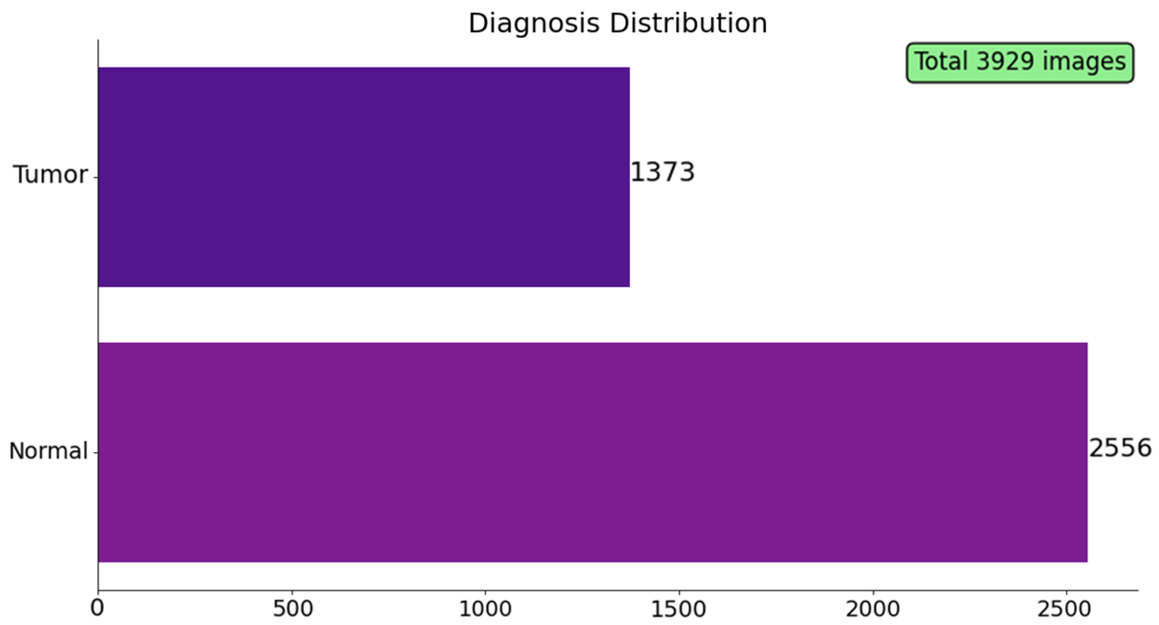
To provide an intuitive grasp of the data fed to the segmentation pipeline, this section walks through a set of descriptive plots and slice-level examples drawn directly from the training files. Figure 2 summarizes the class distribution in the image dataset. Out of 3929 axial FLAIR slices, 2556 (65%) contain no visible tumor signal, whereas 1373 (35%) include at least one pixel annotated as lower-grade glioma.
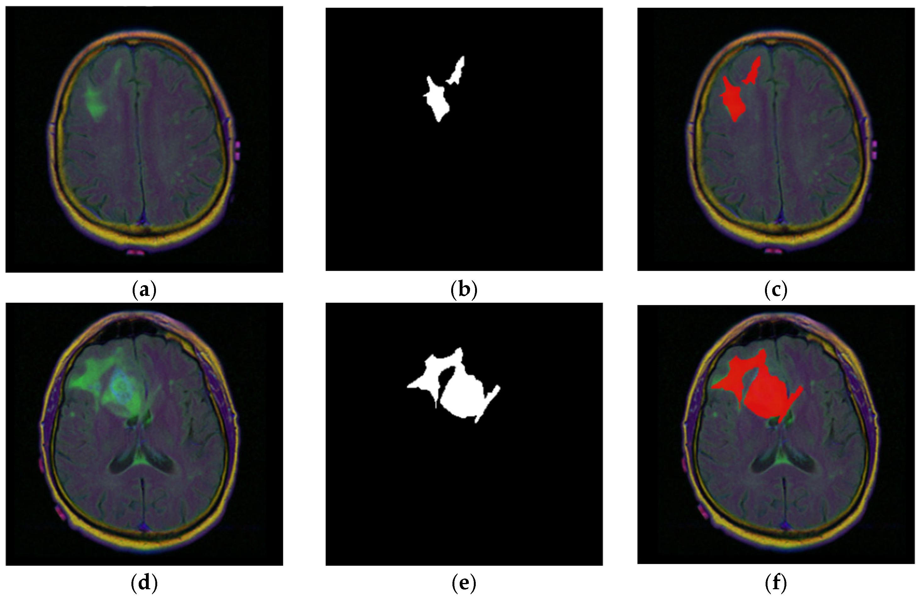
Figure 3a–f zooms in on a single patient, with ID “TCGA_CS_4941_19960909”, to illustrate how expert annotations align with raw images. Figure 3a,d shows two representative FLAIR slices. The corresponding binary masks are displayed in Figure 3b,e, where white pixels mark the tumor footprint. Figure 3c,f overlays mask contours (red) on the original MRIs, highlighting the accuracy of the ground truth masks.
Figure 4a stacks all 23 slices available for the same patient in cranio-caudal order. The sequence reveals how the cranial vault initially appears tumor-free and gradually opens to reveal the lesion, which then enlarges before disappearing again. Figure 4b presents the ground truth masks for those 23 slices without the underlying MRI signal, emphasizing the sparsity of positive pixels in many frames.
Figure 5 combines the two views of Figure 4, overlaying every mask on its corresponding MRI slice-image, reinforcing the spatial coherence of the annotations that will later be used as a qualitative benchmark for model outputs.

3.1.3. Dataset Preprocessing

Before model training, the image dataset was subjected to two complementary splitting strategies followed by identical pixel-level normalization. All steps were implemented using python 3.10, utilizing the PyTorch v2.8.0 framework [48].
The first approach treats every image–mask pair as an independent sample. The dataset was divided as follows: 10% of the 3929 slices were held out for testing and 20% of the remainder for validation, while stratifying on the binary diagnosis label to preserve the tumor/normal ratio across sets. Table 2 highlights that the resulting partition (2750/825/354 samples) is well balanced, with 69.99% of the training images, 21.00% of the validation images and 9.01% of the test images, but slices from the same patient can appear in multiple subsets, a choice that maximizes the number of training examples yet risks optimistic performance because of cross-patient information leakage.
To obtain a more rigorous estimate of generalization to unseen subjects, a second split method was followed and created at the patient level. The 110 patient IDs were shuffled and divided in proportions of 70%, 20%, and 10%, resulting in 79, 20, and 11 patients respectively. All slices from a given patient were kept together, yielding 2828 training, 708 validation and 393 test samples. Although the tumor/normal distribution is slightly different from the slice-stratified split as shown in Table 3 (71.98%/18.02%/10%), this schema eliminates patient overlap between sets and therefore can serve as a benchmark throughout the study. As shown by the experimental results in Section 4.1.1 and Section 4.1.2, the second dataset split approach led to consistently better performance.
During batch generation, and before feeding any image–mask pairs in the tested DL architectures, both images and masks were rescaled to [ 0 ,   1 ] by simple division by 255. Mask arrays are further converted to a two-channel one-hot encoding [ p b a c k g r o u n d ,   p t u m o r ] to suit the softmax output layer and compare with the sigmoid activation function when using the voting mechanism and post-refinement, as described in Section 4.3. Each slice in the data generator is also resized to 256 × 256 pixels, matching the native TIFF resolution.

3.2. Deep Learning Segmentation

Brain-tumor detection is cast here as a binary semantic-segmentation task in which every axial FLAIR slice is mapped to a mask that labels each pixel as tumor or background. Two fully-convolutional encoder–decoder networks are explored, U-Net [22] and its Attention-augmented variant [49], because they combine global context (captured by progressive down-sampling) with the fine detail needed to follow the irregular lesion borders.
To investigate how the choice of output layer affects segmentation performance and to provide suitable outputs for post-processing, two versions of both the U-Net and Attention U-Net backbones were used. In the first version, the final 1 × 1 convolution outputs a single logit per pixel, followed by a sigmoid activation, producing a continuous confidence score in the range [ 0 ,   1 ] . While suitable for binary segmentation, this representation lacks information about background confidence and is therefore less useful for uncertainty-aware post-processing. In the second version, the network outputs two logits per pixel, followed by a softmax activation, yielding normalized probabilities for both background and tumor classes. This dual-class confidence gives the opportunity to be later exploited by the slice-to-slice voting scheme mechanism as well as the post-heuristic refinement steps. Keeping both heads therefore lets us contrast a standard segmentation pipeline with one explicitly designed to preserve per-pixel uncertainty for post-processing.

3.2.1. U-Net Architecture

The network follows the original four-level design introduced by Ronneberger et al. (2015) [22] with some alterations. The contracting path consists of successive 3 × 3 convolutions, rectified-linear activations and batch normalization; channel depth doubles after each 2 × 2 max-pool, progressing 64, to 128, to 256, to 512, to 1024 filters at the bottleneck. The expanding path mirrors this structure: every up-convolution doubles the spatial size and halves the channel count, after which the corresponding encoder feature map is concatenated to restore fine detail. Two convolutions refine the merged tensor before the next up-sample. A final 1 × 1 convolution projects the 64-channel map to either one or two logits as outlined above. With an input of 256 × 256 × 3 the model contains just above 31 M trainable parameters yet fits comfortably in GPU memory thanks to its strict 2D design, striking a balance between capacity and computational efficiency.
This symmetrical topology has two advantages in the current setting: (i) it can be trained from scratch on datasets of only a few thousand slices without severe overfitting; and (ii) its skip connections prevent the loss of small structures.
Figure 6 presents an overview of the four-level U-Net used in this study. Blue–green boxes on the left form the encoder: each block halves the spatial resolution, from 256 to 16 pixels, while doubling the number of feature channels, from 64 gradually to 1024. Yellow–blue boxes on the right form the decoder: transposed-convolution (“UpConv”) blocks restore resolution back to 256 × 256 while successively halving channel depth. Dashed grey arrows indicate skip connections that copy high-resolution features from the encoder to the decoder; solid arrows denote the main forward path. Furthermore, Figure 6 shows the two different U-Net approaches with two output heads: one with a single-channel sigmoid and one with a two-channel softmax.

3.2.2. Attention U-Net Architecture

Attention U-Net retains the depth, filter sizes and skip topology of the vanilla U-Net architecture but inserts a learnable Attention Gate (AG) on every encoder–decoder shortcut. Each AG receives (i) the semantic context emerging from the decoder at a given scale and (ii) the fine, localization-rich features streamed from the matching encoder layer. Through a lightweight gating mechanism composed of 1 × 1 convolutions, element-wise addition, a single sigmoid activation and up-sampling, the gate generates a spatial attention coefficient α 0 , 1 256 × 256 that modulates the encoder features before fusion [49]. Consequently, irrelevant or noisy regions are weakened, while spots likely to belong to the tumor are emphasized, and all with only a small computational overhead of less than 5%.
Figure 7 represents the Attention U-Net variant, which keeps the standard U-shape of the baseline U-Net but adds AGs on every skip connection.

3.3. Deep Learning Segmentation Model Training

Images and masks were provided to the network by a paired generator that kept the two perfectly aligned, while applying random basic geometric augmentations. Each slice was checked to be 256 × 256 pixels, converted to floating-point, and normalized to the [ 0 , 1 ] range. Data augmentation introduced gentle variation: small rotations, horizontal and vertical shifts of 5%, shear of 5%, and zoom of 5%. These settings were chosen after small pilot runs showed that stronger distortion did not improve validation accuracy.
Both U-Net and Attention U-Net were trained for 100 epochs with a batch size of 8. Weight tensors were initialized with the recommended variance-preserving scheme for ReLU layers, and all models were optimized with Adam, with a learning rate of 1 ×   10 4 . Adam optimizer [50] was preferred over Stochastic Gradient Descent (SGD) [51] because preliminary experiments produced higher training and validation scores. The learning rate followed a simple linear decay schedule that reached zero at the final epoch. No explicit weight decay or dropout was required to control over-fitting.
To explore the influence of the objective function, each architecture was trained three times: once with Dice loss [40], once with Dice and Binary Cross-Entropy (DiceBCE), and once with focal Tversky loss [52]. Masks were encoded as two channels when the network used the softmax head and as a single channel when the sigmoid head was selected, so that each loss received inputs in its preferred format.

3.4. Evaluation Metrics

The cancer area segmentation problem entails a classification problem for which a set of specific metrics are used [25] for their ability to highlight different viewpoints of pixel-level performance. In particular, six measures are reported: accuracy, precision, recall, Intersection-over-Union (IoU), F1-score and the Area Under the ROC Curve (AUC). Accuracy captures overall agreement, precision reflects specificity, recall measures sensitivity, IoU emphasizes spatial overlap, the F1-score combines precision and recall into a single value, and AUC provides a threshold-independent view of class separability.
The metrics are defined from the confusion-matrix counts of True Positives (TP), True Negatives (TN), FP and False Negatives (FN) as follows:
A c c u r a c y = T P + T N T P + T N + F P + F N
P r e c i s i o n = T P T P + F P
R e c a l l = T P T P + F N
F 1 S c o r e = 2 × P r e c i s i o n × R e c a l l P r e c i s i o n + R e c a l l = 2 × T P 2 × T P + F P + F N
I o U = T P T P + F P + F N
AUC is obtained by varying the decision threshold across the full [ 0 ,   1 ] range, plotting the TP rate against the FP rate, and computing the area under the resulting curve; it can be interpreted as the probability that a random tumor pixel receives a higher confidence score than a random background pixel.

4. Results

4.1. Assessment of Deep Learning Segmentation Models

Before presenting the qualitative results, the analysis is split into two subsections, Section 4.1.1 and Section 4.1.2, which investigate the influence of the output-layer activation. Section 4.1.1 focuses on models that generate a sigmoid confidence map, whereas Section 4.1.2 examines the corresponding softmax variants. The comparison establishes whether any segmentation accuracy is sacrificed when the softmax activation function is adopted as head for the post-heuristic refinement described later in Section 4.3.

4.1.1. Assessment of Sigmoid Output Layer Architectures

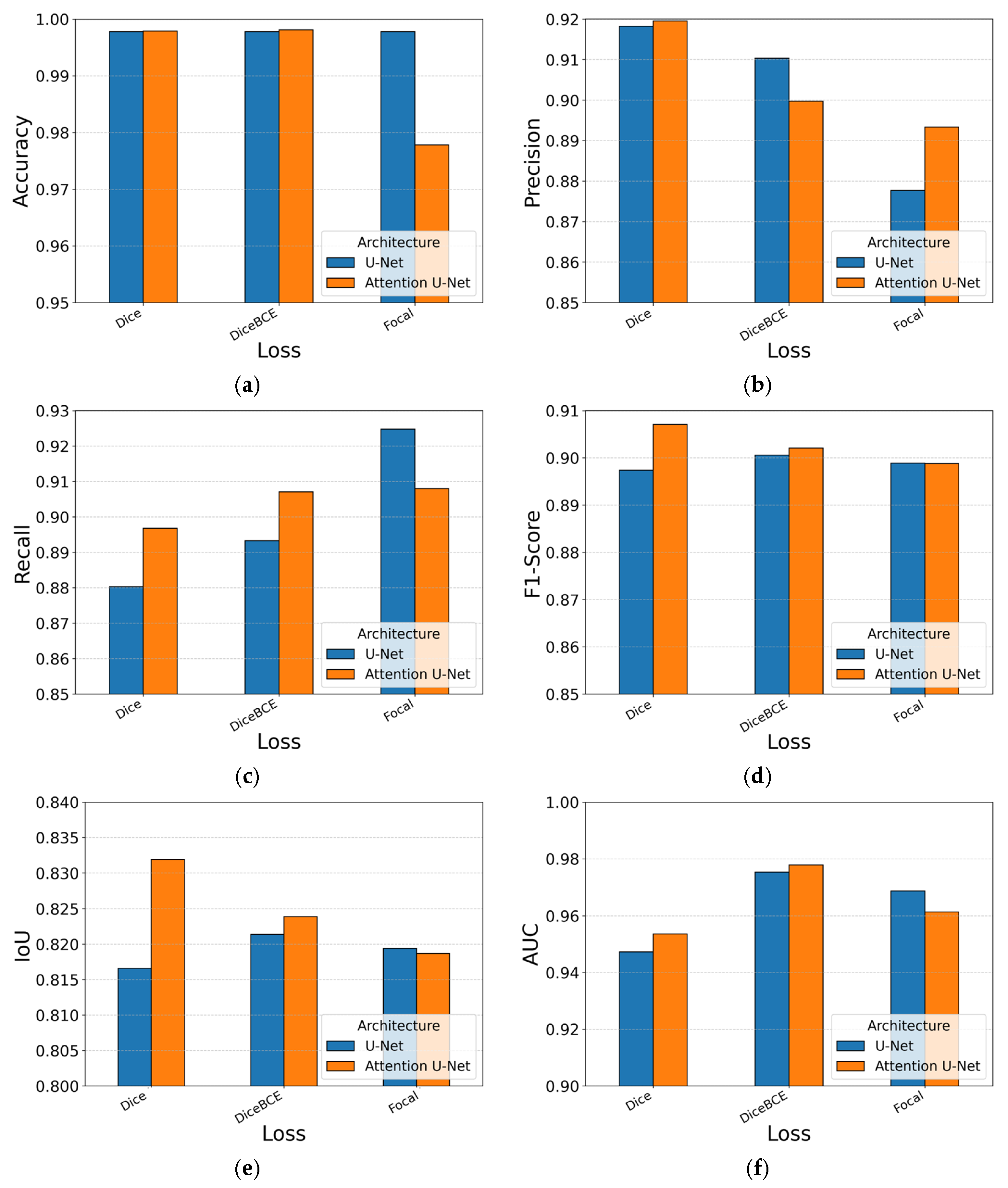
Table 4 reports the metric scores and Figure 8 visualizes the same data for easier comparison. Across all runs, the absolute performance is high, pixel accuracy remains above 0.95 and AUC above 0.94, yet clear patterns emerge. Introducing AGs consistently improves localization: relative to the baseline U-Net, the Attention U-Net raises all metrics when paired with Dice loss. The gains are small in magnitude but appear in every metric, confirming that the AGs help the decoder emphasize tumor pixels without inflating FPs.
The choice of loss function modulates this behavior. Pure Dice loss delivers the strongest segmentation scores, F1-Score and IoU peak at 0.907 and 0.831 with the Attention U-Net. Focal loss shifts the trade-off toward recall on both architectures (0.9248 with U-Net and 0.908 with Attention U-Net) but lowers precision and, consequently, overall accuracy; the emphasis on hard examples appears less beneficial when false-positive control is essential.
In terms of training dynamics, focal loss generally requires close to the full 100 epochs, whereas the other two losses seem to be able to converge even 20–25% sooner. Figure 8 reinforces the narrative: orange columns, which represent Attention U-Net, sit just above their blue counterparts for most losses, while Dice columns dominate the IoU and F1-score subfigures.
Taken together, the experiments single out the Attention U-Net trained with pure Dice loss as the most balanced performer, offering the best combination of segmentation, sensitivity and specificity. This result is obtained when using the second dataset split method where all slices from a single patient strictly belong to only one subset. The first split strategy, where patient slices could appear in multiple subsets, yielded inferior results in all cases and is included solely as a baseline reference in the underlined row of Table 4. It is important to highlight that the slice-wise split, where slices from the same patient may appear in multiple subsets, suffers from cross-patient leakage and may overestimate the performance, so it should be reported only as a baseline. When threshold-independent discrimination or shorter training times are paramount, the DiceBCE configuration provides a compelling alternative without a meaningful drop in segmentation quality.
Figure 9 illustrates the learning dynamics of the best-performing Attention U-Net trained with a sigmoid head and Dice loss. Figure 9a depicts the normal route for both sets, with training error falling sharply during the first ten epochs and then tapering toward a stable value of 0.10, while the validation curve follows the same trajectory with small, noise-like fluctuations; the absence of a widening gap indicates neither overfitting nor underfitting. Figure 9b tracks the IoU, which climbs quickly above 0.75 and stays at around 0.82 for the remainder of training, while Figure 9c shows an almost identical course for the F1-Score, levelling off close to 0.90. The close alignment of the blue (training) and orange (validation) traces in all three graphs confirms that the model generalizes well and that the best metric scores at epoch 71 were captured on the flat part of each curve.
Comprehensive learning curves for every U-Net and Attention U-Net configuration with a sigmoid output layer are provided in Appendix A. Figure A1 and Figure A2 replicate the layout of Figure 9, showing that the same stable convergence pattern holds across all loss functions.

4.1.2. Assessment of Softmax Output Layer Architectures

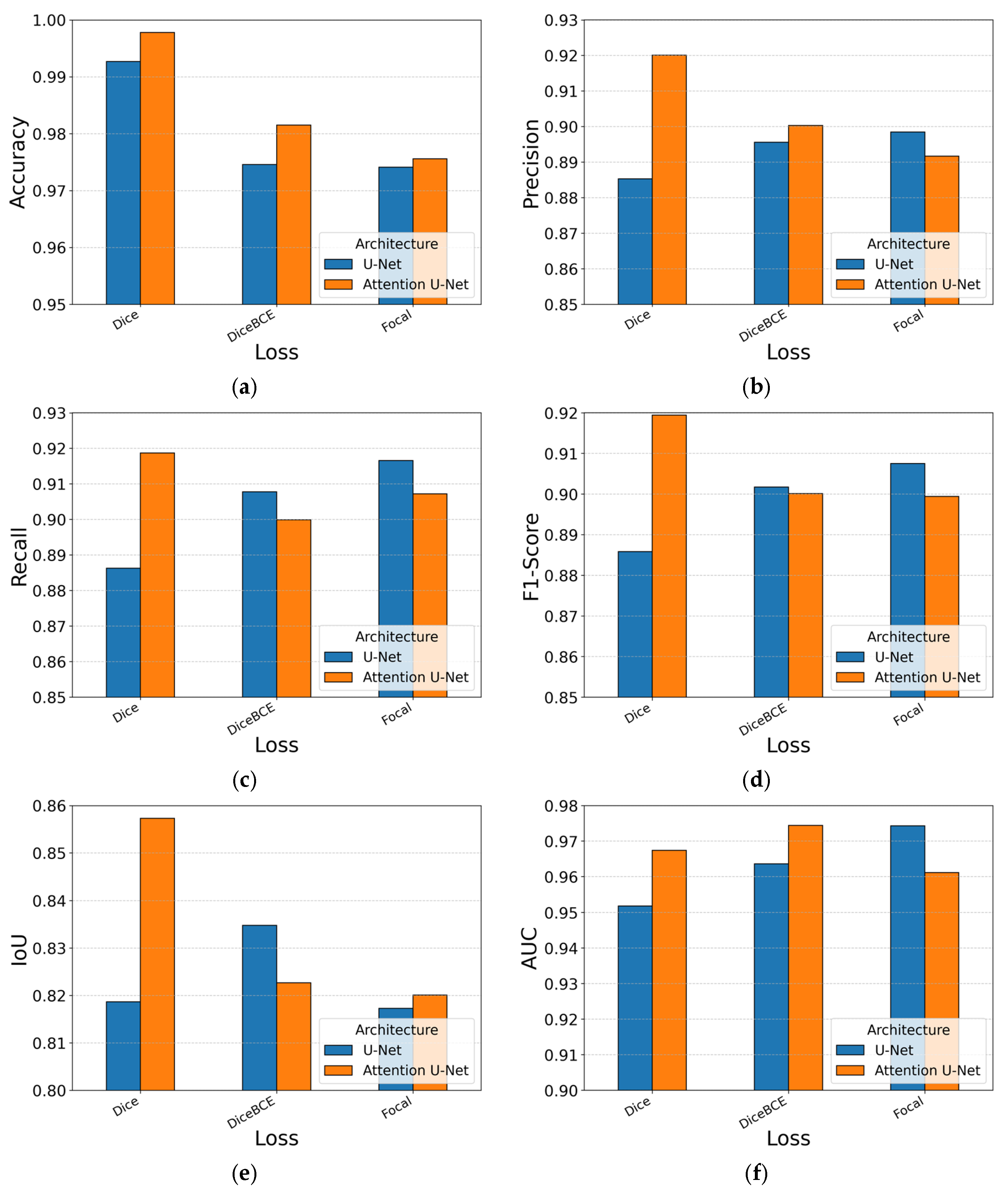
Table 5 lists the quantitative scores obtained when the architectures are defined with a two-channel softmax activation function output. Figure 10a,f reproduces the same results graphically. All combinations again reach high absolute performance, accuracies stay above 0.97 and AUC above 0.95, but, as with the sigmoid head, clear differences appear between architectures and loss functions. Replacing the plain U-Net with its Attention-Gated counterpart remains beneficial: with Dice loss, the Attention U-Net raises precision to 0.920 and recall to 0.918, pushing the F1-Score to 0.919 and IoU to 0.857, the best values obtained with softmax. DiceBCE and focal losses behave similarly to the sigmoid setting: DiceBCE balances precision and recall but yields a slightly lower IoU, while focal loss achieves higher recall at the expense of precision and overall accuracy.
Training times follow the same pattern. Models trained with focal loss usually run close to the full 100 epochs, whereas DiceBCE variants converge after roughly three quarters of the schedule. The best softmax model, Attention U-Net combined with Dice loss, achieved an IoU of 0.857 at epoch 76. This result corresponds to the second dataset split method, where each patient’s slices are confined to a single subset. As with the sigmoid output layer experiments in Section 4.1.1, the first split strategy, that allowing patient slices to appear in multiple subsets, consistently led to lower performance and is included only as a baseline reference in the underlined row of Table 5.
Visual inspection of Figure 10 confirms these patterns. The orange columns representing Attention U-Net sit above the blue columns for most metrics when Dice loss is used, whereas the gaps narrow or reverse for DiceBCE and focal loss. In particular, the Dice bars dominate the F1-Score and IoU plots, reinforcing the conclusion that Dice loss remains the best choice for this particular segmentation task.
Figure 11 illustrates the learning curves for the best performing model. Figure 11a shows that training and validation loss fall rapidly during the first ten epochs, then settle near 0.12 with only small fluctuations, indicating stable optimization. Figure 11b,c showcases IoU and F1-Score, where both metrics climb steadily past 0.80 within the first 25 epochs and remain flat thereafter, with the two traces almost overlapping. The tight alignment of training and validation curves, again, confirms good generalization and the absence of under- or overfitting to the training data.
Comparing the two activation strategies, the softmax head neither improves nor degrades segmentation quality in a meaningful way: the best IoU with softmax (0.857) is within one percentage point of the corresponding sigmoid result, and the rank ordering of losses is unchanged. Because IoU is the principal selection criterion throughout this work, the Attention U-Net trained with Dice loss is retained as the reference model for the refinement experiments in Section 4.3. Full training curves for every softmax run are provided in Appendix A, where Figure A3 and Figure A4 replicate the format of Figure 11 for completeness.

4.2. Qualitative Results

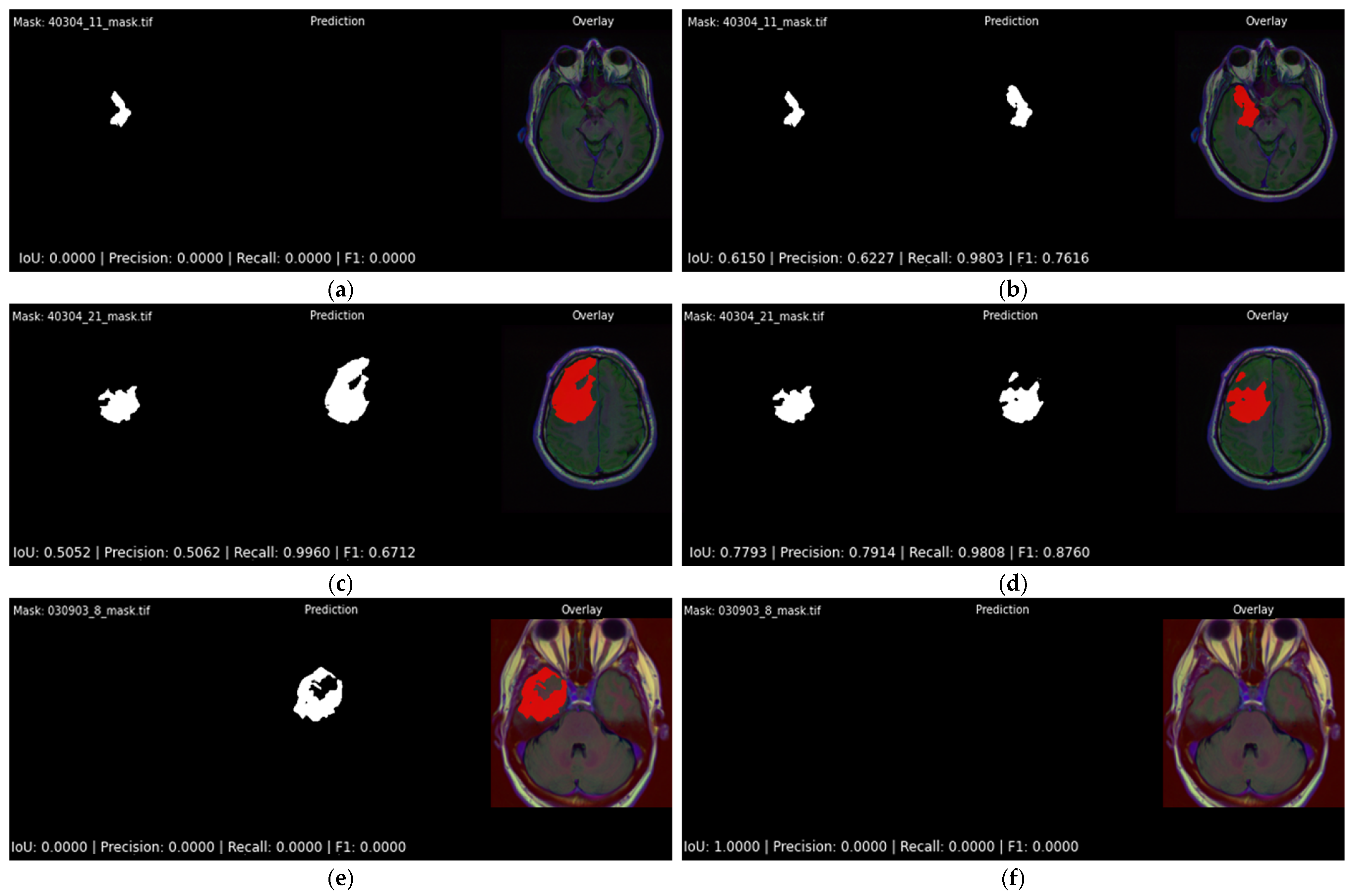
Figure 12 offers a side-by-side visual comparison of the two best-performing configurations as reported in Table 4 and Table 5, Attention U-Net trained with DiceBCE loss, under the two alternative output layers. The left column, Figure 12a,c,e, shows the sigmoid variant, while the right column, Figure 12a,c,e, shows the softmax variant. Each horizontal row represents the same patient, so differences between columns isolate the influence of the activation alone. The first row highlights a particularly challenging slice containing a very small lesion. The sigmoid model is unable to mark any overlapping pixels with the ground truth mask, which represents the worst possible detection outcome in a clinical setting (FN). The softmax model, although far from perfect, does identify part of the lesion and achieves an IoU of 0.615 (Figure 12b), demonstrating a clear practical advantage. The second row follows the same pattern: both models detect the bulk of the tumor, but the softmax head yields a noticeably higher overlap with the ground truth mask (IoU 0.779 versus 0.505). In the final row of Figure 12, where the ground truth mask does not contain any tumor pixels, the softmax variant accurately predicts this, whereas the sigmoid output falsely contains many tumor pixels. These examples confirm the quantitative finding that, although the two activations are statistically close, the softmax variant is less likely to fail catastrophically on difficult slices.
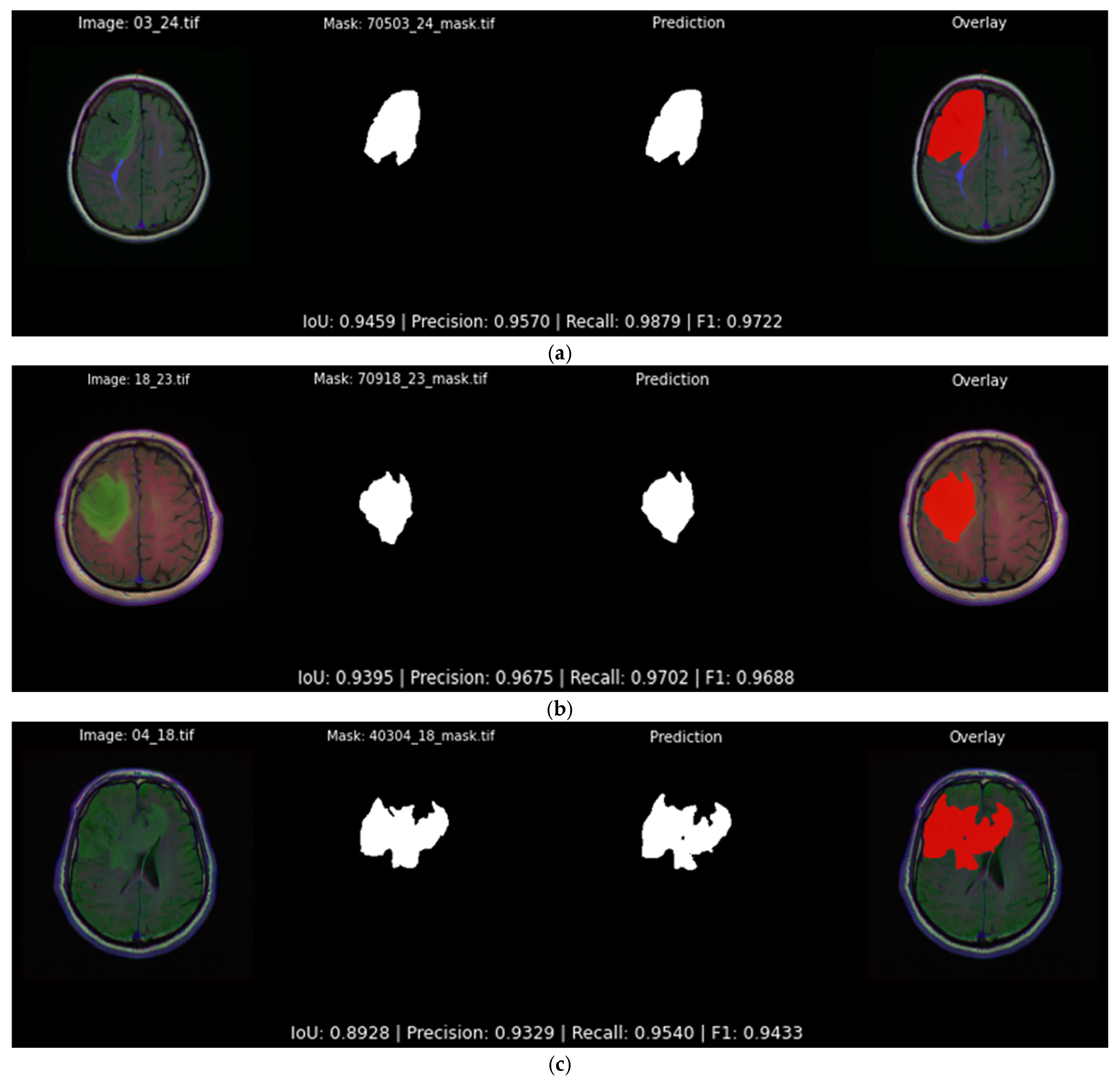
Figure 13 illustrates three typical highly accurate segmentations predicted by the best-performing softmax model presented in Table 5. All predictions follow the tumor boundaries closely, with IoU scores of 0.946, 0.940 and 0.892 for each example, respectively. In each case, the predicted mask aligns with the ground truth, not only predicting its general shape but also most of the details.
Conversely, Figure 14 showcases three examples in which the same model struggles, where irregular tumor shapes lead to fragmented or under-segmented predictions. The first and second slices still achieve moderate IoU values just below 0.60, yet noticeable portions of the tumor are missing. The third slice showcases the most challenging amongst the examples of Figure 14, where the network detects only a small fragment of the ground truth region, yielding an IoU of 0.378. Such cases highlight the inherent difficulty of the precise tumor segmentation and motivate the post-processing refinements described later in Section 4.3.
To complement the visual inspection, Table 6 summarizes the major qualitative findings, providing a concise overview of the observations described above in Figure 12, Figure 13 and Figure 14.

4.3. Voting Mechanism and Post-Heuristic Segmentation Refinement

The quantitative evaluation in Section 4.2 shows that even the best-performing 2D Attention U-Net occasionally produces implausible slice-wise tumor masks, from tiny false-positive island pixels to abrupt volume increases, or complete miss-detections in some slices. Because tumor voxels evolve smoothly along the craniocaudal axis and every patient axial MRI contains tens of contiguous axial FLAIR images, meaning that slices are not independent, we exploit inter-slice anatomical continuity to rectify such inconsistencies with a two-stage strategy. The pipeline of the strategy is composed of (i) a voting mechanism that exploits the white-area overlap percentage between MRIs, measuring how much the tumor area on one slice overlaps with its immediate neighbor and (ii) a post-heuristic refinement that uses the per-pixel softmax confidences to reduce low-confidence ambiguous pixels in the descending area of the overlap curve and after its peak.

4.3.1. White-Area Overlap Between Sequential Slices

As every patient has a stack of contiguous axial MRI images, successive slices inevitably share a portion of the same tumor tissue, especially around the center of the lesion. Quantifying how much of the tumor footprint persists from one slice to the next therefore constitutes a natural first step. We measure this persistence as the White-Area Overlap percentage (WAO) between consecutive slices, computed for both the ground truth annotations and the model predictions.
Let M i and M i + 1 denote the binary tumor masks of slices i and i + 1 either originating from ground truth annotation or from the model prediction. For two consecutive slices i and i + 1 the WAO is computed as follows:
W A O i , i + 1 = | M i M i + 1 | M i × 100 % ,
where | | counts foreground pixels. Equation (1) is asymmetric on purpose: it answers the clinical question, “How much of the current tumor cross-section persists in the next slice?” A value of 100% indicates that the tumor footprint of slice i is fully contained in slice i + 1 , whereas 0% implies no spatial overlap. The procedure is summarized in Algorithm 1.
Algorithm 1 Calculation of White-Area Overlap (WAO) between two slices
Input: Binary tumor masks M i and M i + 1
Output: Overlap percentage W A O i , i + 1
1: Identify all foreground (tumor) pixel in slice M i .
2: Count how many of these pixels are also tumor in slice M i + 1 .
3: Compute overlap percentage:
W A O i , i + 1 = | M i M i + 1 | M i × 100 %
4: If slice M i contains no tumor pixels then set W A O i , i + 1 = 0
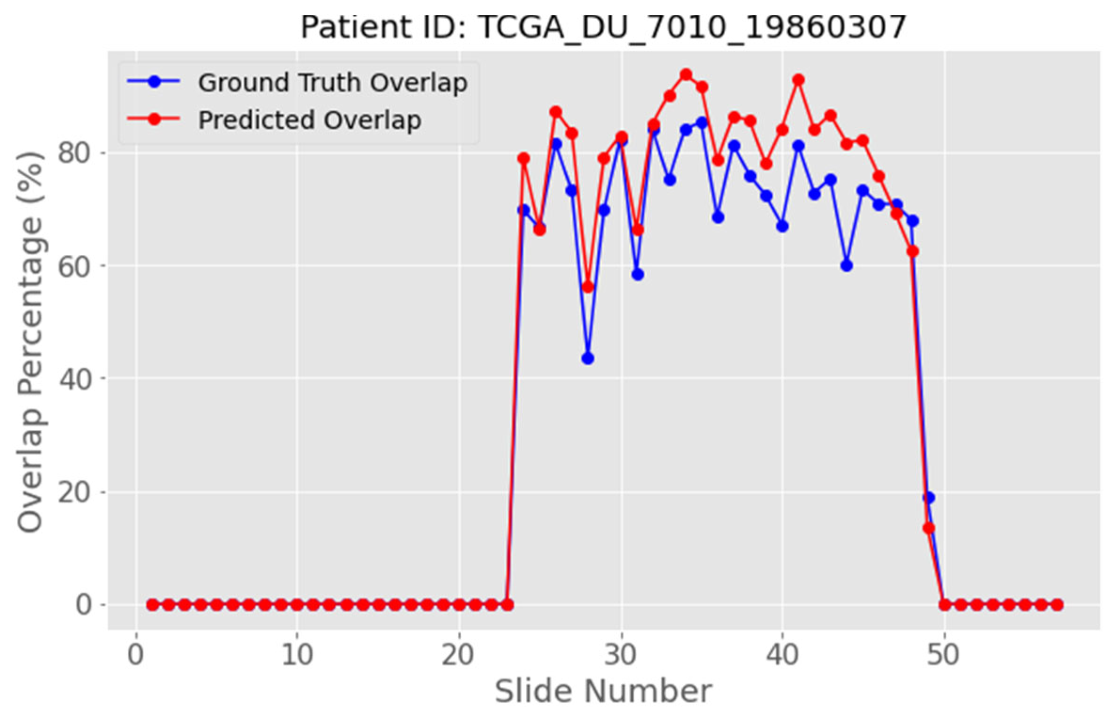
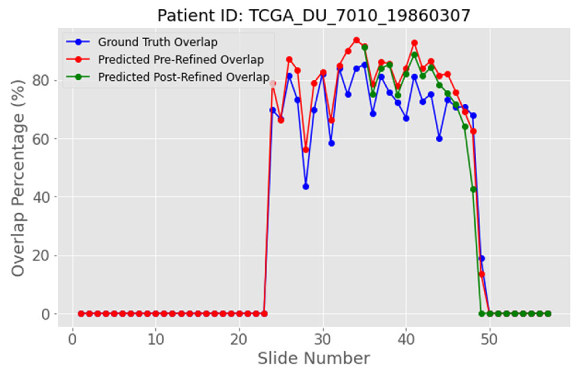
Plotting WAO against the slice index yields a bell-shaped curve that climbs as the tumor gradually appears, reaches a maximum close to the largest lesion cross-section, and descends as the tumor vanishes, as shown in the blue curve of Figure 15. The red curve shown in Figure 15 represents the predicted white overlapping pixels. We exploit this characteristic shape to delineate three anatomical regions: pre-peak (rising limb), peak slice, and post-peak (falling limb). Figure 15 illustrates this behavior clearly. In most of the starting slices, the WAO remains essentially 0%, because tumor tissue is still absent; the curve then rises steeply as the acquisition reaches the lesion core, attains a single maximum at the peak slice, and finally descends as the stack progresses and the tumor vanishes. During the rising limb, each successive slice is expected to contain more tumor pixels than its predecessor, whereas after the peak the opposite trend most likely holds, and each new slice should exhibit fewer tumor pixels. Detecting this peak, visible in the blue ground truth curve of Figure 15, is crucial as it anchors the definition of the pre-peak, peak, and post-peak regions that underpin the refinement strategy, described in the following sections. Of course, as shown in Figure 15, the near peak region contains WAO values that are extremely close to its value. Therefore, from a clinical standpoint, the aim is to identify the narrow neighborhood of slices in which the lesion attains its largest cross-section, rather than to single out one exact WAO value for a single slice.

4.3.2. Peak Localization of White-Area Overlap via Gaussian Smoothing

The raw WAO series derived from both the ground truth and the softmax predictions displays high-frequency fluctuations (blue and red curve of Figure 15). To obtain a robust estimate of the WAO peaks, we smooth the series with a 1D Gaussian filter ( σ = 2 ) :   w ~ = g σ w where g σ is a discrete Gaussian kernel and denotes convolution. The peak index is then i = a r g m a x i w ( i ) .
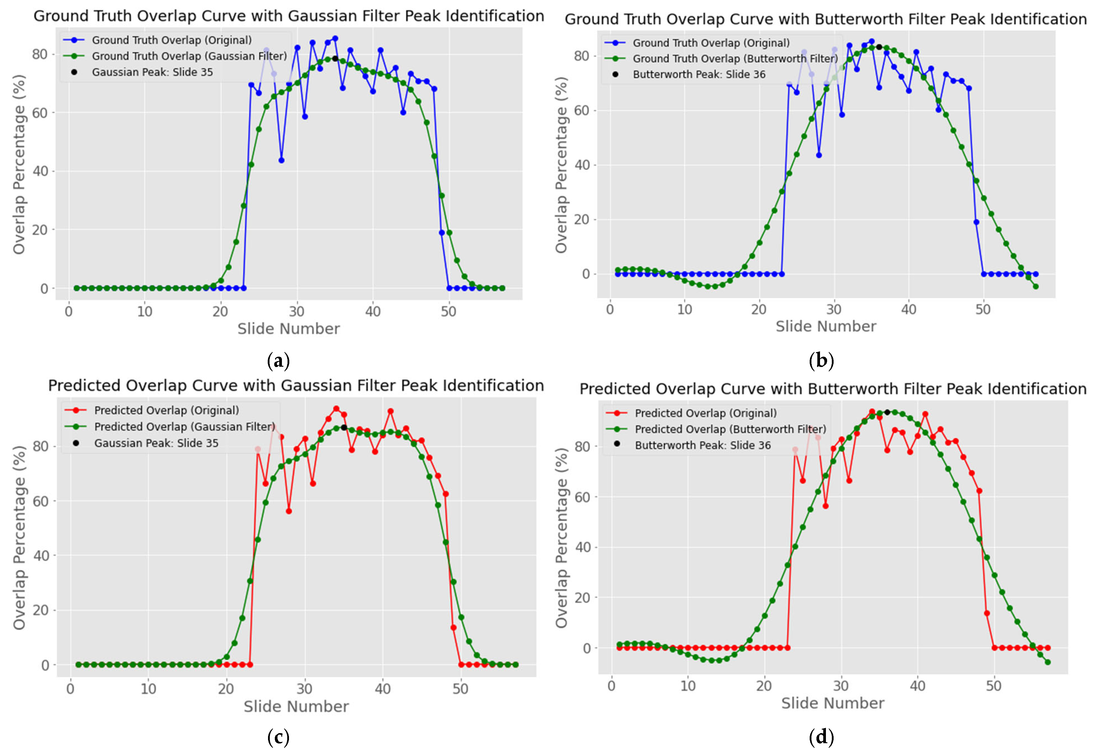
The suitability of the Gaussian kernel was evaluated against a fifth-order Butterworth low-pass filter with a normalized cut-off frequency of 0.1. For every subject in the study cohort Ν = 110 , six peak positions were extracted: the peak of the raw ground truth WAO curve, the peaks obtained after Gaussian and Butterworth smoothing of that ground truth curve, and the equivalent three peaks computed from the model predicted WAO curve. These values are shown in Table A1 of Appendix B.
The absolute deviation between each smoothed peak and its corresponding reference peak was then grouped into error bands of 0, 1 and 2 slices; the resulting counts are summarized in Table A2. Gaussian smoothing located the peak within ± 2 slices of the reference in 85 out of 110 ground truth curves (77.3%) and in 68 out of 110 predicted curves (61.2%), whereas the Butterworth filter achieved the same tolerance in 53 cases (48.2%) and 60 cases (54.5%), respectively. Gaussian smoothing also produced more exact matches, with 18 ground truth curves showing zero-slice deviation compared with 12 for the Butterworth alternative. These observations confirm that the Gaussian kernel preserves the location of broad maxima while effectively suppressing local fluctuations, and it is therefore adopted for peak localization in all subsequent experiments.
Figure 16a in conjunction with the blue curve of Figure 15 shows the correct peak identification at slice number 35 when using the Gaussian filter, where in Figure 16b the peak is calculated at slice number 36 when using the Butterworth filter. On the other hand, Figure 16c,d represents the equivalent peak identifications for the same patient but now for the predicted masks, where both filters do not accurately pinpoint the exact peak but a neighboring slide. However, as previously mentioned, the identification of the narrow neighborhood of slices in which the lesion attains its largest cross-section is achieved.

4.3.3. Heuristic Refinement of Ambiguous Softmax Pixels

Once the peak slice i has been identified, the predicted WAO curve reveals in which part of the slides the network tends to over-segment or under-segment the tumor volume. Both errors arise mainly from pixels whose class probabilities are almost tied. Our heuristic therefore acts only on ambiguous pixels, shifting them either to background or to tumor depending on the sign of the error.
Let p 0 x , y ,   p 1 x , y be the softmax probabilities for background and tumor, and define the class-gap map d x , y = p 1 x , y p 0 x , y [ 1,1 ] . Pixels with | d | close to zero are deemed ambiguous. For every slice j > i , we sort the flattened d values and peak a slice-specific threshold τ j = Q u a n t i l e ρ ( d x , y ) , with ρ ( 0,100 ) .
Ambiguous removal strategy (Section Removal of Ambiguous Softmax Pixels) is applied if the refined WAO must decrease, where all pixels with d ( x , y ) τ j are re-labelled as background by setting p 1 0 ,   p 0 1 . On the other hand, ambiguous addition strategy (Section Addition of Ambiguous Softmax Pixels) is applied if the refined WAO must increase, where all pixels with d ( x , y ) τ j are promoted to tumor ( p 1 1 ,   p 0 0 ). In both cases the map is renormalized so that p 0 + p 1 = 1 . A default value of ρ = 0.1 3 % works well across patients, but of course can be tuned when necessary. Further results can be found in Section 4.4.
Removal of Ambiguous Softmax Pixels
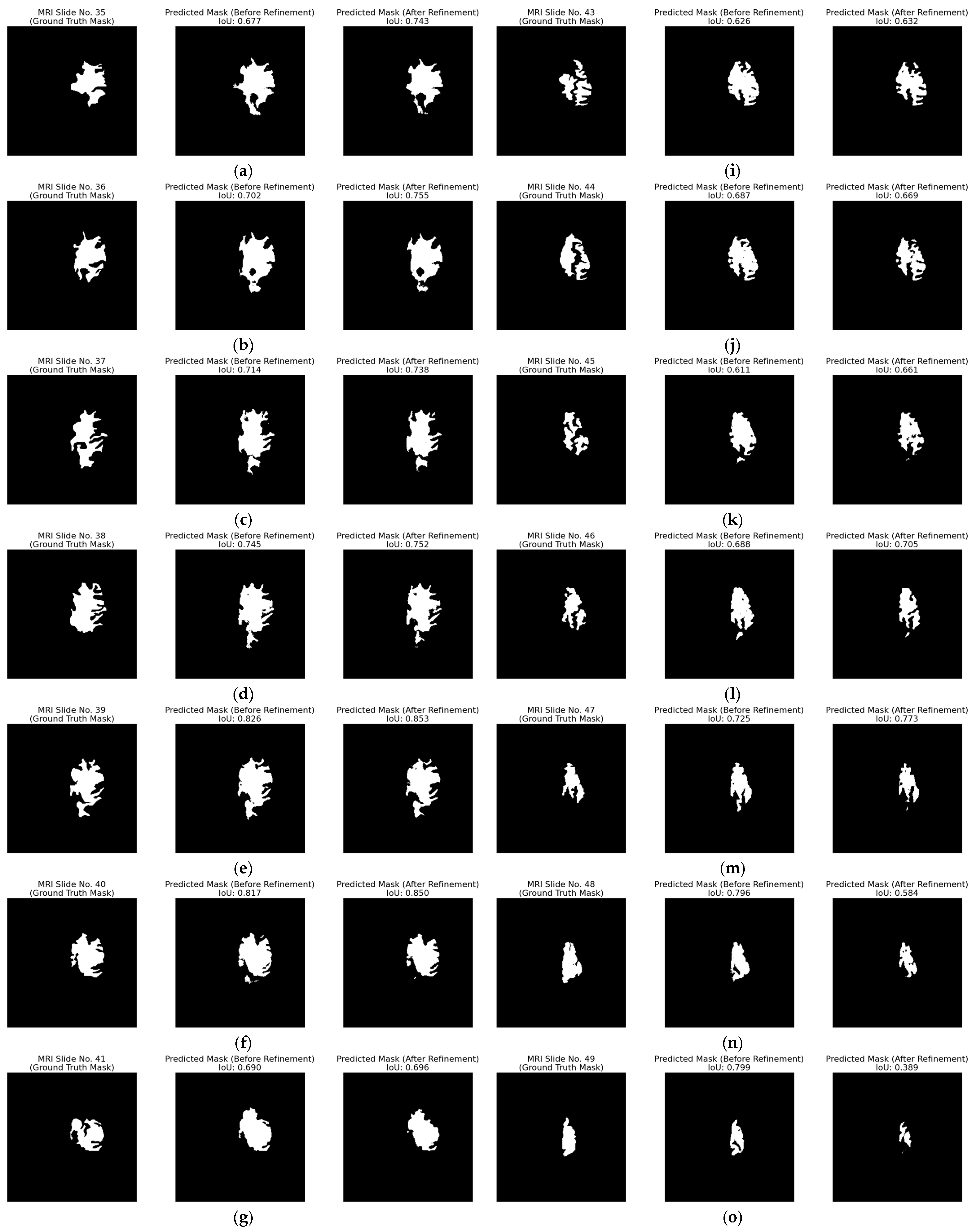
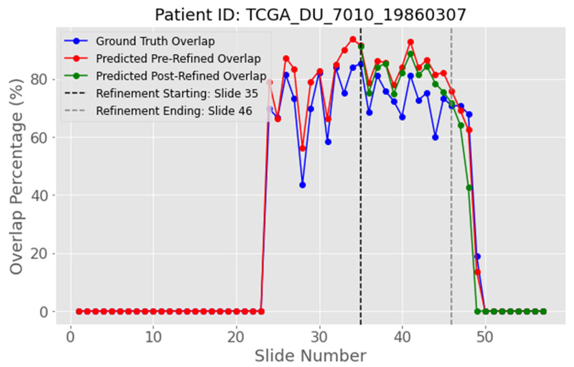
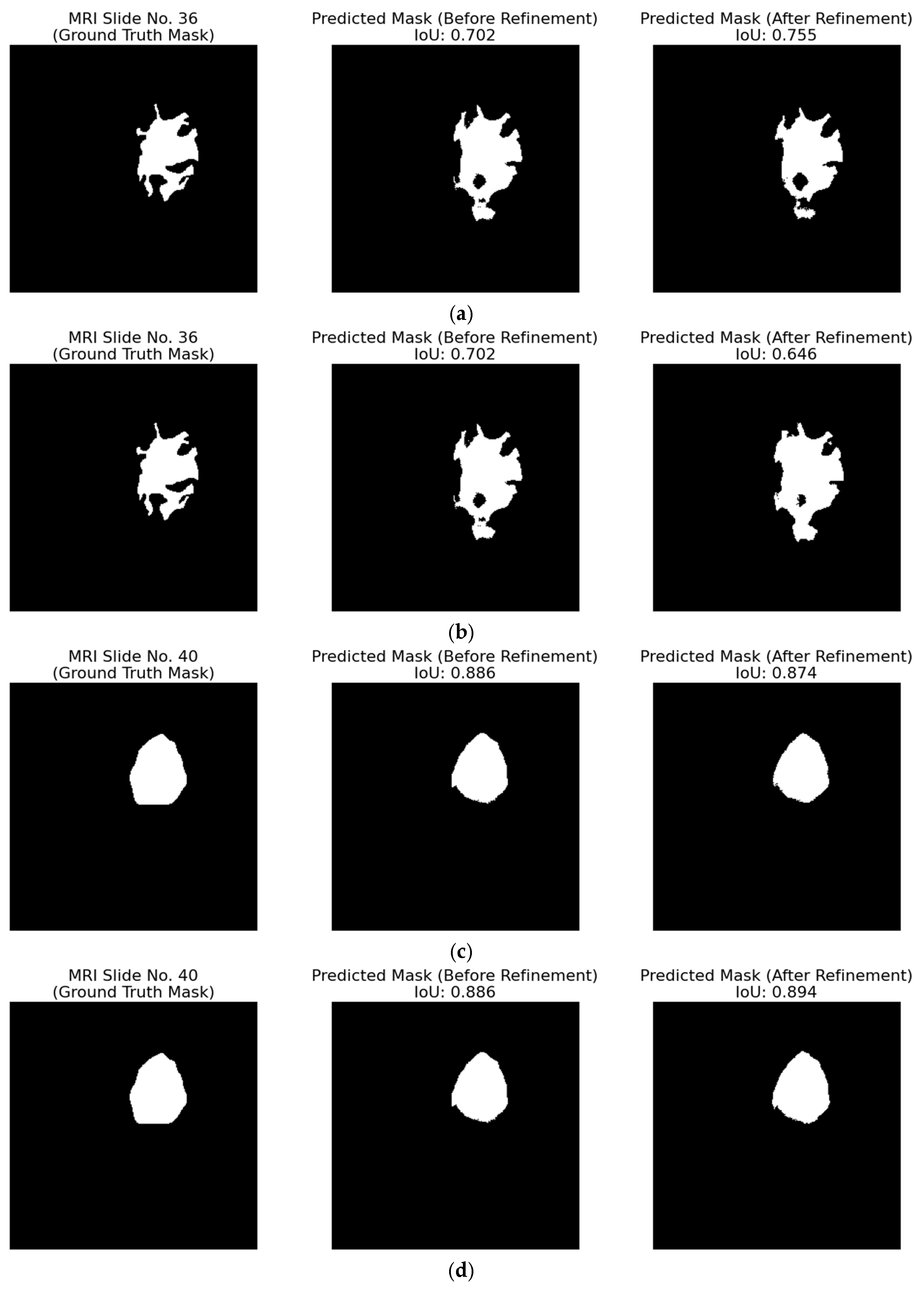
The strategy of removing ambiguous pixels that fall below a fixed percentage threshold and re-labelling them as background is evaluated on patient with ID “TCGA_DU_7010_19860307”. In Figure 17, the red curve, which shows the predicted overlap before refinement, sits well above the blue ground truth curve. After ambiguous-pixel removal with a threshold of 1.5%, the green curve moves between the other two, coming closer to ground truth. This positive result is also evident in most of the subfigures in Figure 18, where the IoU of the predicted mask after refinement is clearly improved. For example, in Figure 18a,b, the IoU increased from 0.677 to 0.743 and from 0.702 to 0.755, respectively.
However, Figure 18p exposes an important failure case. An MRI slice with an initial low IoU of 0.594 contains a small tumor region that disappears completely when 1.5% of ambiguous pixels are set to background, producing an FN, which is the worst possible outcome in a clinical setting.
In order to avoid this issue and further improve the results of the post-heuristic refinement, we introduce an early-stop rule that limits refinement to the slices where it is helpful. The stopping point is found by locating the first sharp drop in the Gaussian-smoothed overlap curve. Figure 19 shows that, for this patient, the drop occurs at slide 46, thus creating an area of 12 slides (35 to 46) to which the refinement is applied.
The results of this effect are evident in Table 7. Refining every slice lowered the mean IoU (mIoU) from 0.799 to 0.761, but restricting refinement to the selected window raises IoU by almost 2%, giving a clear improvement for this patient.
Addition of Ambiguous Softmax Pixels
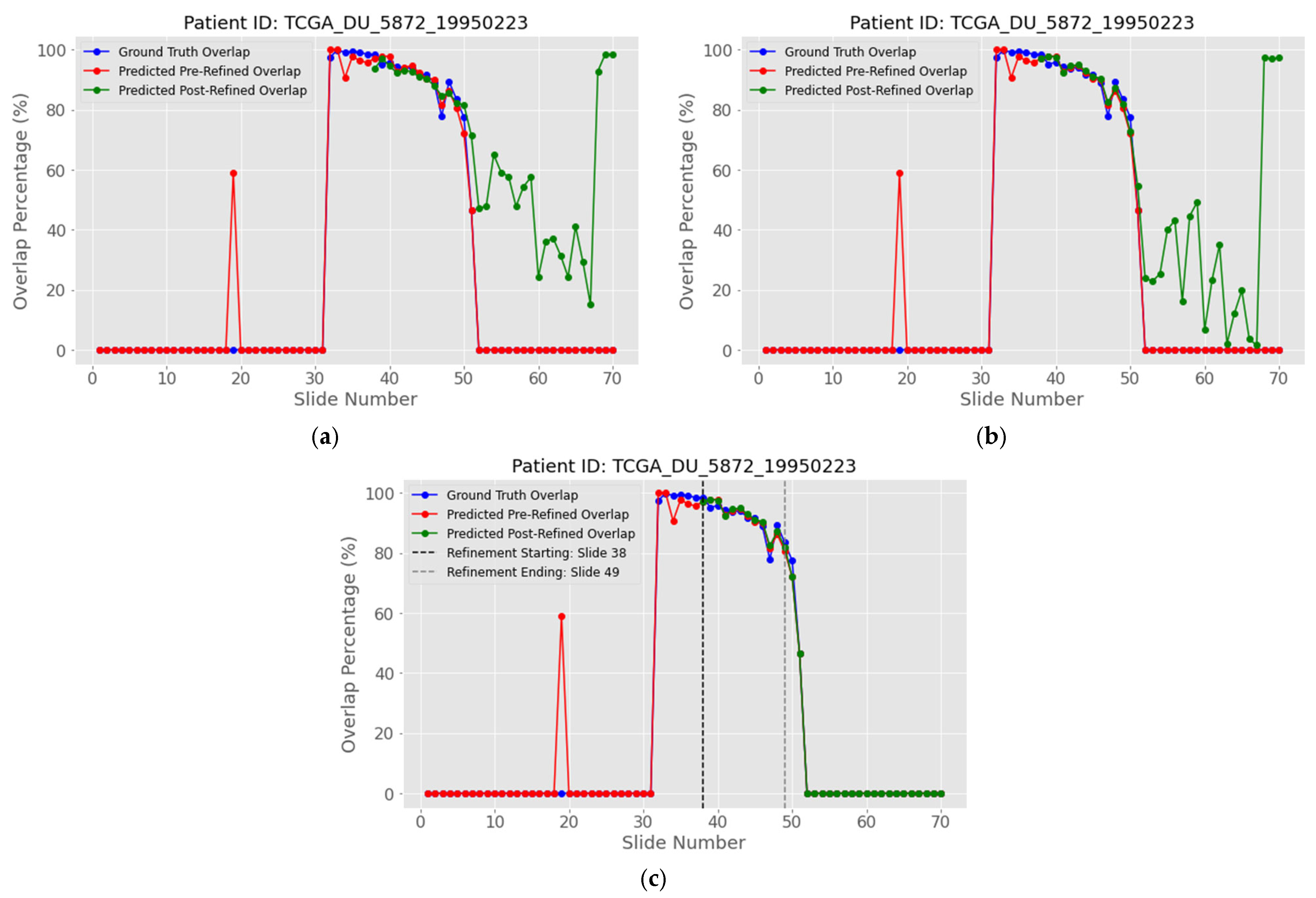
The complementary approach, re-labelling a small fraction of ambiguous pixels as tumor, is analyzed and shown on patient with ID “TCGA_DU_5872_19950223”. More specifically, Figure 20a show that the green curve, obtained after adding 1.5% of the most ambiguous pixels to the tumor class, stays below both the ground truth (blue) and the unrefined prediction (red) for much of the stack, indicating persistent under-segmentation. Beyond roughly slice 51, the same curve crosses above the others, meaning that the 1.5% threshold now introduces too many tumor pixels. To balance these effects, Figure 20b reduces the threshold to 0.3%, and Figure 20c further restricts refinement to the slices identified by the stopping rule introduced earlier. The isolated red spike at slice 19 stems from a small prediction error in the predicted mask because, but because the refinement window begins later, this anomaly is left unchanged.
Figure 21a,c shows how the 1.5% threshold negatively affects this case, where white pixels are added, leading to a worse IoU per MRI slide. For this reason, a smaller value of 0.3% was investigated for this patient, in which Figure 21b,d shows a significant improvement in the IoU metric from 0.899 to 0.922 and from 0.878 to 0.885, respectively.
Table 8 highlights the importance for both hyper-parameters, percentage threshold and slide window of applying the refinement strategy. The baseline IoU of 0.914 drops sharply with an addition of tumor pixels with a 1.5% threshold, recovers partially when 0.3% is introduced, and improves by a further 4.5% (0.956) when the refinement window is restricted, underscoring the need to tune both the percentage and the application range.
Figure 22 illustrates how the two refinement rules behave on representative slices. For patient with ID “TCGA_DU_7010_19860307”, Figure 22a shows that removing 1.5% of the most ambiguous pixels raises IoU from 0.702 to 0.755, whereas Figure 22b shows that adding 1.5% ambiguous pixels on the same slice degrades IoU to 0.626. The opposite occurs for patient with ID “TCGA_DU_5872_19950223” under a 0.3% threshold: Figure 22c indicates that removal reduces IoU from 0.886 to 0.874, while Figure 22d shows that addition improves IoU from 0.886 to 0.894. These examples confirm that the percentile and the choice between removal or addition must be adapted to the patient/slide context.

4.4. Assessment of the Holistic Approach of Voting Mechanism and Post-Heuristic Refinement

Having analyzed the two refinement strategies individually, ambiguous-pixel removal and ambiguous-pixel addition, we now assess their aggregate impact across the entire patient cohort. The key questions are (i) whether either strategy improves the model’s predictions on a population level, (ii) by how much, and (iii) under which threshold settings the benefit is obtained.
Table 9 investigates these points for all patients in the dataset, reporting the mIoU value before and after refinement, for every tested threshold (3% to 0.1%), separately for the removal and addition procedures, with the refinement always confined to the patient-specific window defined in Section 4.3.3. The right-most column lists the number of patients whose individual IoU improves under each setting. From the results presented, it is quite clear that a consistent pattern emerges for both strategies: as the threshold percentage decreases, performance of mIoU improves, highlighting that only the most ambiguous pixels should be re-labelled. Crucially, the entire refinement step executes in roughly 2 s per patient volume, so these gains come at no significant runtime cost.
The standout result of Table 8 comes from the removal strategy at thresholds of 0.3%, 0.2% and 0.1%. At these settings the post-refinement mIoU surpasses the baseline value of 0.815, reaching 0.816, 0.825 and 0.832, respectively, while benefitting 56, 61 and 67 patients. Although the absolute gains are modest, they clearly demonstrate the potential of discarding a tiny fraction of highly ambiguous pixels to mitigate FPs, a promising avenue for future work, as discussed in Section 5.
By contrast, the addition refinement strategy yields a lower mIoU than the baseline at every threshold, even though it helps up to 32 individual patients. This suggests that pronounced under-segmentation, such as the patient case detailed in Section Addition of Ambiguous Softmax Pixels, is comparatively rare. Consequently, ambiguous-pixel addition should not be discarded outright, but future research should first identify patients who exhibit systematic under-segmentation and apply the method selectively to that subgroup.

5. Discussion and Future Work

Several factors temper these encouraging results. The refinement rules rely on hand-set thresholds (e.g., 0.1–3%) tuned retrospectively; although coarse grid-searches were performed, no principled mechanism adapts these values to unseen cases. Second, the WAO peak is detected on a per-patient basis, so errors in peak localization, or highly irregular tumors without a clear bell-shaped overlap, propagate to the refinement stage. Finally, the ambiguous addition strategy never lifted mIoU above baseline in our experiments, highlighting its sensitivity to patient-specific under-segmentation that the current heuristic cannot predict.
It should also be noted that, for the two dataset splits that were examined in Section 3.1.3, for any claim about model performance, only the patient-wise split provides a valid estimate of generalization because all slices from a subject remain in a single subset, eliminating cross-subject information leakage. In contrast, the slice-wise split can place near-duplicate slices from the same volume in both training and test sets. This leakage lets the network memorize patient-specific anatomy and routinely inflates output metric scores, a well-known pitfall in medical-imaging ML. Consequently, slice-wise results in this work are reported solely as a methodological baseline and are not interpreted as indicative of real-world performance on unseen patients.
This study reports single-cohort results on TCGA-LGG without an external test set; therefore, generalizability to other institutions, scanners, vendors, acquisition parameters, or clinical populations remains unknown. In medical imaging, distributional shifts (e.g., intensity/contrast differences, slice thickness, reconstruction kernels, annotation style, disease mix) can materially affect CNN performance. The figures reported here should thus be interpreted as within-cohort estimates. Robust external validation [53] on multi-center datasets and stress-testing across different protocol variations are required before clinical deployment [54].
Performance comparison to other approaches requires a careful setup which allows for the same resources and a solid data split prior to any training and validation. Such a task was outside of the scope of this research, but can be considered as a follow-up work.
Another aspect that should be noted is that this study adopts a patient-wise hold-out split to estimate generalization. We acknowledge that patient-level k-fold cross-validation would provide a tighter estimate of performance variance and reduce dependence on any single partition. We chose hold-out for two practical reasons: (i) computational cost, training and evaluating the full pipeline (including post-heuristic analysis) across multiple folds would increase complexity; and (ii) alignment with intended use, training on a large portion of the cohort and testing on a disjoint patient set mirrors deployment more closely. Nonetheless, hold-out estimates can be split-sensitive; results should therefore be interpreted as within-cohort performance on this partition.
Future research should address these limitations in three directions: (i) adaptive refinement: replace fixed percentile thresholds with uncertainty-aware schemes that tune the ambiguous pixel fraction dynamically per slice; (ii) patient stratification: develop pre-filters that flag under-segmented cases, perhaps via global volume discrepancy, so that ambiguous pixel addition is applied selectively;’ and (iii) cross-site evaluation, data harmonization, and domain-adaptation strategies to improve out-of-distribution robustness. Furthermore, after achieving this stratification, a hybrid refinement strategy could be applied, where both ambiguous pixel additions and removals are taken into consideration.

6. Conclusions

This study set out to improve lower-grade-glioma segmentation in axial FLAIR MRI by combining an efficient 2D Attention U-Net with a lightweight slice-to-slice refinement pipeline. After benchmarking two network backbones (vanilla and Attention U-Net) under three loss functions and two output activations, the Attention U-Net trained with Dice loss and a softmax head emerged as the most balanced performer, achieving a mIoU of 0.857 on a patient-wise hold-out set of 110 TCGA-LGG subjects.
The paper’s main contribution is a lightweight voting-and-refinement scheme that leverages inter-slice anatomy without introducing trainable parameters or 3D computation. To alleviate the occasional slice-wise inconsistencies typical of 2D models, the voting mechanism measures the WAO between neighboring slices and localizes its peak via a Gaussian filter smoothing. Exploiting this bell-shaped WAO curve, a post-heuristic refinement suppresses or augments low-confidence pixels only in the post-peak region. Two complementary rules are evaluated: (i) ambiguous-pixel removal, which re-labels a small percentage of near-tie softmax pixels as background, and (ii) ambiguous-pixel addition, which promotes an equally small fraction to the tumor class. An early-stop criterion based on the first sharp WAO drop limits refinement to the neighborhood where it proved beneficial.
Cohort-level analysis (Table 9) demonstrates that this targeted parameter-free post-processing can improve the baseline produced by the best 2D model. In particular, small removal thresholds (0.3–0.1%) consistently lift the cohort mIoU above the baseline from 0.815 (baseline) to 0.832, while improving up to 67 individual patients; addition helps selected under-segmented cases when applied with conservative thresholds inside the WAO-derived window. The refinement step adds only about 2 s of processing time per patient, keeping the complete pipeline fast enough without any significant runtime cost.
Overall, the study contributes (i) an interpretable WAO-based voting signal for slice-wise consistency, (ii) a validated Gaussian peak-localization strategy, and (iii) a practical, percentile-driven refinement that improves coherence with minimal overhead. These design choices offer a clear path to more robust 2D MRI segmentation when 3D training or inference is impractical.

Author Contributions

Conceptualization, E.P. and P.C.; methodology, E.P. and P.C.; software, E.P. and P.C.; validation, E.P. and P.C.; formal analysis, E.P. and P.C.; investigation, E.P.; resources, E.P. and P.C.; data curation, E.P. and P.C.; writing—original draft preparation, E.P. and P.C.; writing—review and editing, E.P. and P.C.; visualization, E.P. and P.C.; supervision, E.P. and P.C.; project administration, E.P. and P.C.; funding acquisition, E.P. and P.C. All authors have read and agreed to the published version of the manuscript.

Funding

The APC was funded by the University of Macedonia Research Committee.

Institutional Review Board Statement

Not applicable.

Informed Consent Statement

Not applicable.

Data Availability Statement

The dataset utilized in this study is the “Brain MRI segmentation” https://www.kaggle.com/datasets/mateuszbuda/lgg-mri-segmentation (accessed on 9 July 2024) obtained from Kaggle.

Acknowledgments

This paper is a result of research conducted within the MSc in Artificial Intelligence and Data Analytics of the Department of Applied Informatics of University of Macedonia.

Conflicts of Interest

The authors declare no conflicts of interest.

Abbreviations

The following abbreviations are used in this manuscript:
AGAttention Gate
AIArtificial Intelligence
AUCArea Under the ROC Curve
CNNsConvolutional Neural Networks
CTComputed Tomography
DLDeep Learning
DiceBCEDice and Binary Cross-Entropy
FLAIRFluid-Attenuated Inversion-Recovery
FNFalse Negative
FPFalse Positive
IoUIntersection-over-Union
LGGsLower-Grade Gliomas
MRIMagnetic Resonance Imaging
SGDStochastic Gradient Descent
TCGAThe Cancer Genome Atlas
TCIAThe Cancer Imaging Archive
TNTrue Negative
FPTrue Positive
WAOWhite-Area Overlap
WHOWorld Health Organization

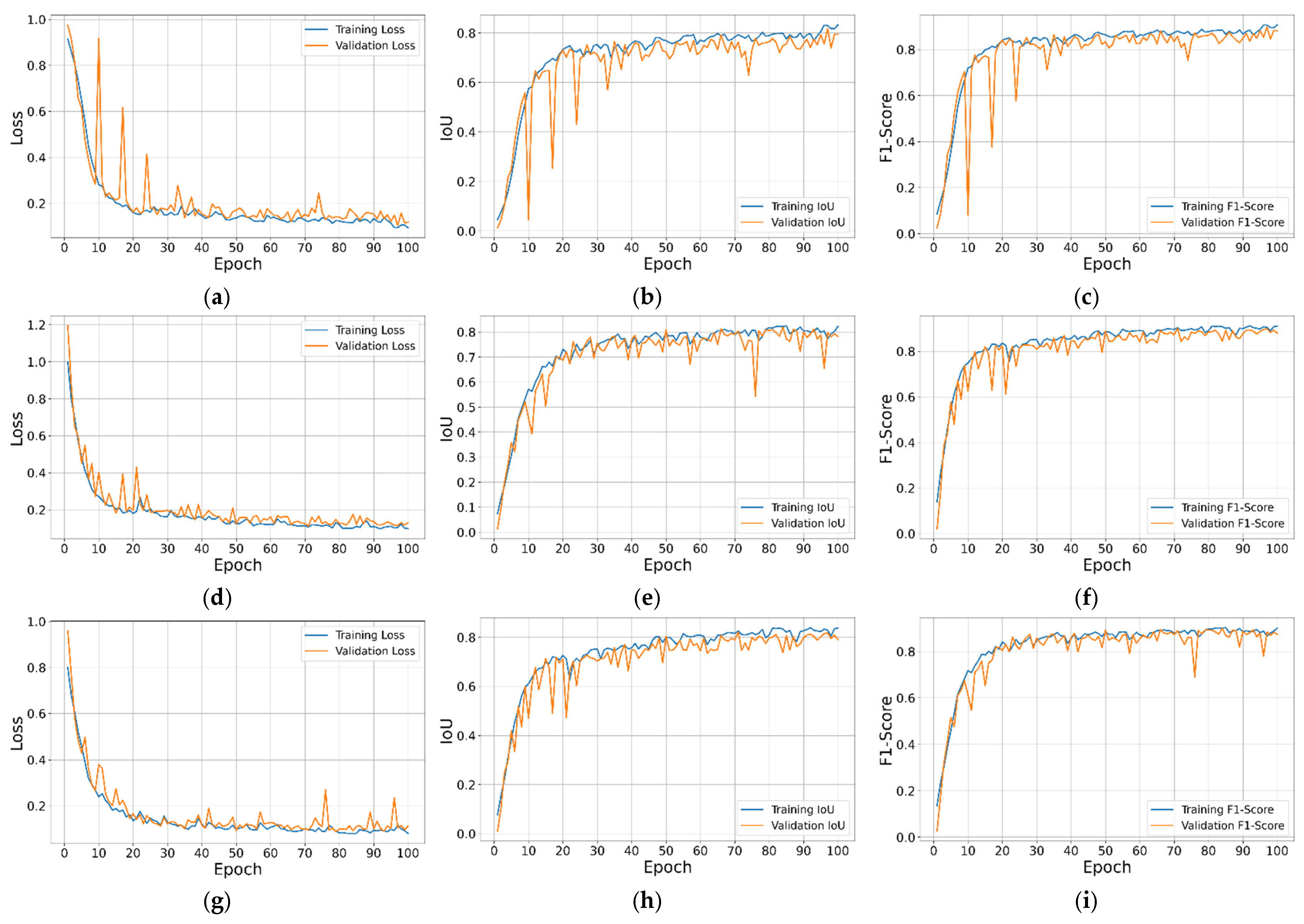
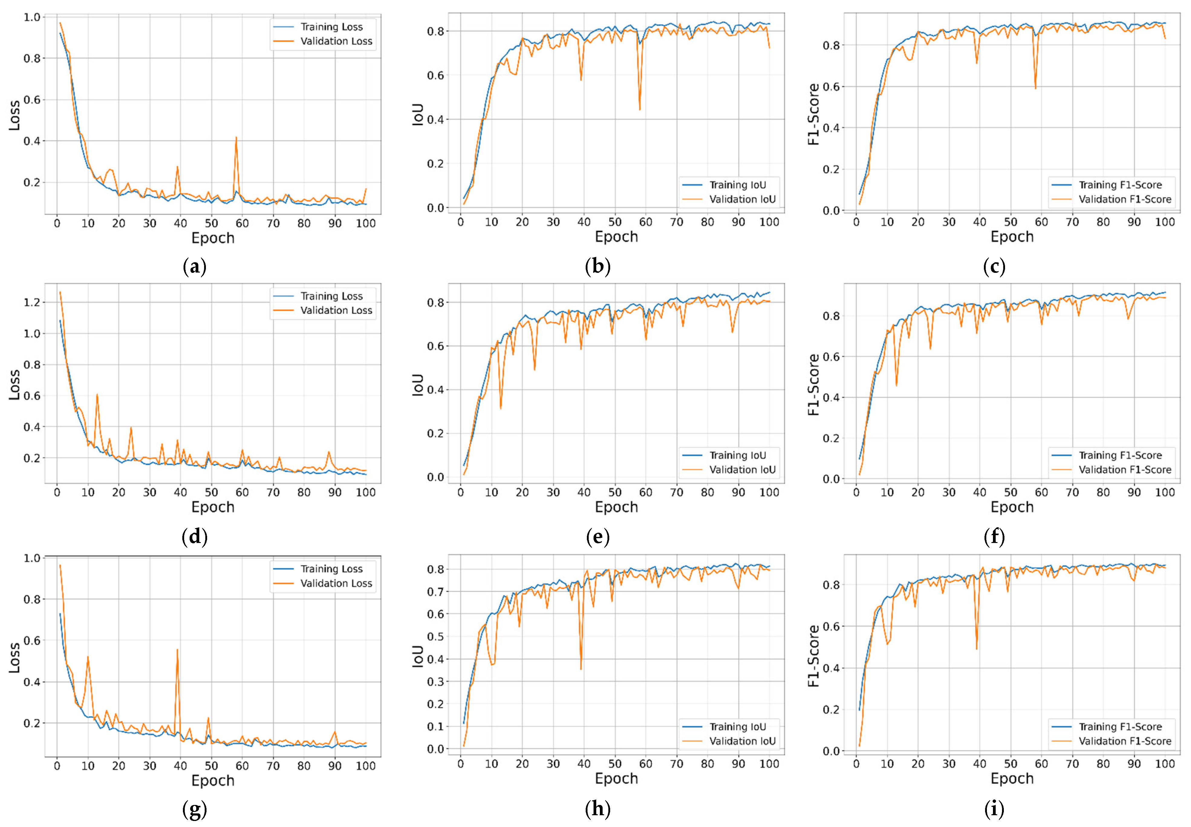
Appendix A

This appendix presents a comprehensive breakdown of segmentation result metrics per epoch for both U-Net and Attention U-Net architectures, coupled with all used loss functions for both sigmoid and softmax activation function approaches. Figure A1 and Figure A2 visualizes the training and validation loss, F1-Score and IoU progression across epochs for the trained U-Net and Attention U-Net models with sigmoid activation function, respectively.
Figure A1. Training and validation loss, IoU, and F1-Score per epoch results for the trained U-Net models with sigmoid output layer: (ac) U-Net with Dice Loss; (df) U-Net with Dice BCE Loss; (gi) U-Net with Focal Loss.
Ai 06 00212 g0a1
Figure A2. Training and validation loss, IoU, and F1-Score per epoch results for the trained Attention U-Net models with sigmoid output layer: (ac) Attention U-Net with Dice Loss; (df) Attention U-Net with Dice BCE Loss; (gi) Attention U-Net with Focal Loss.
Ai 06 00212 g0a2
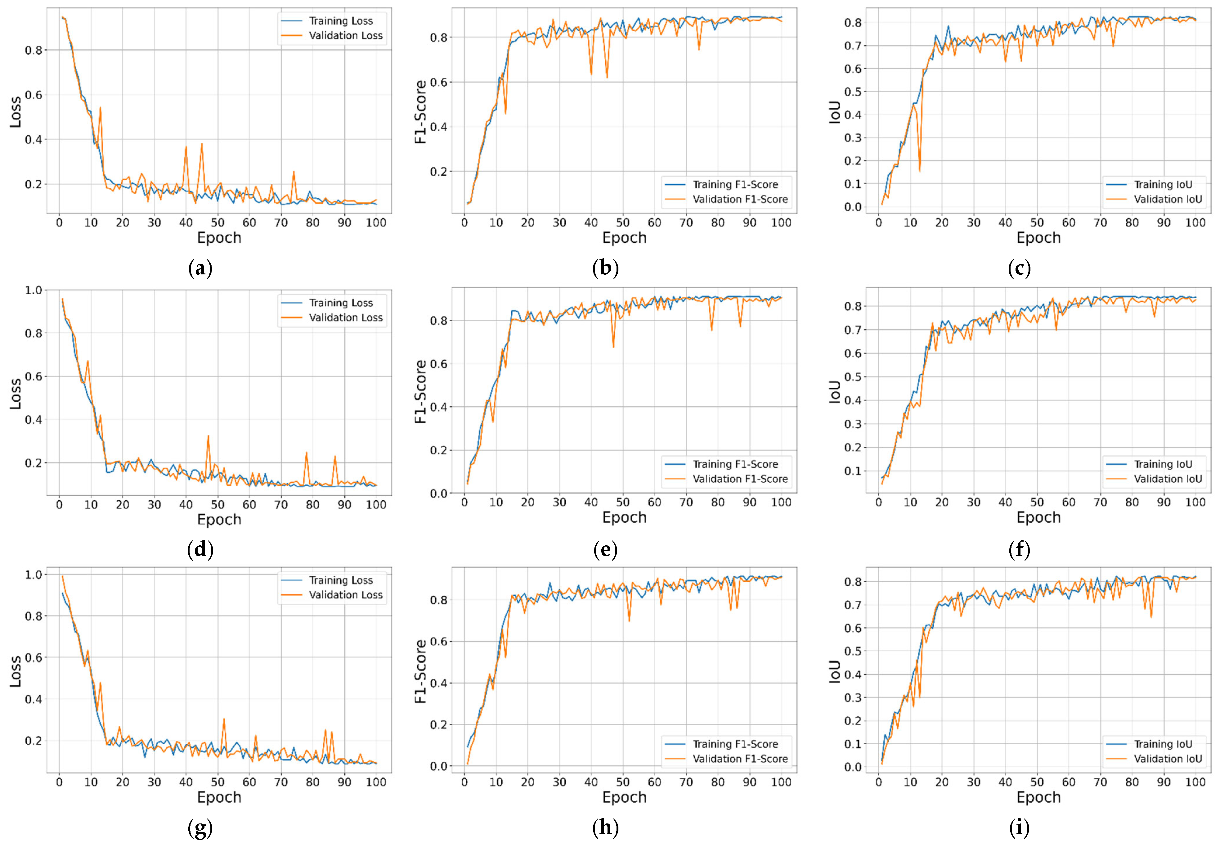
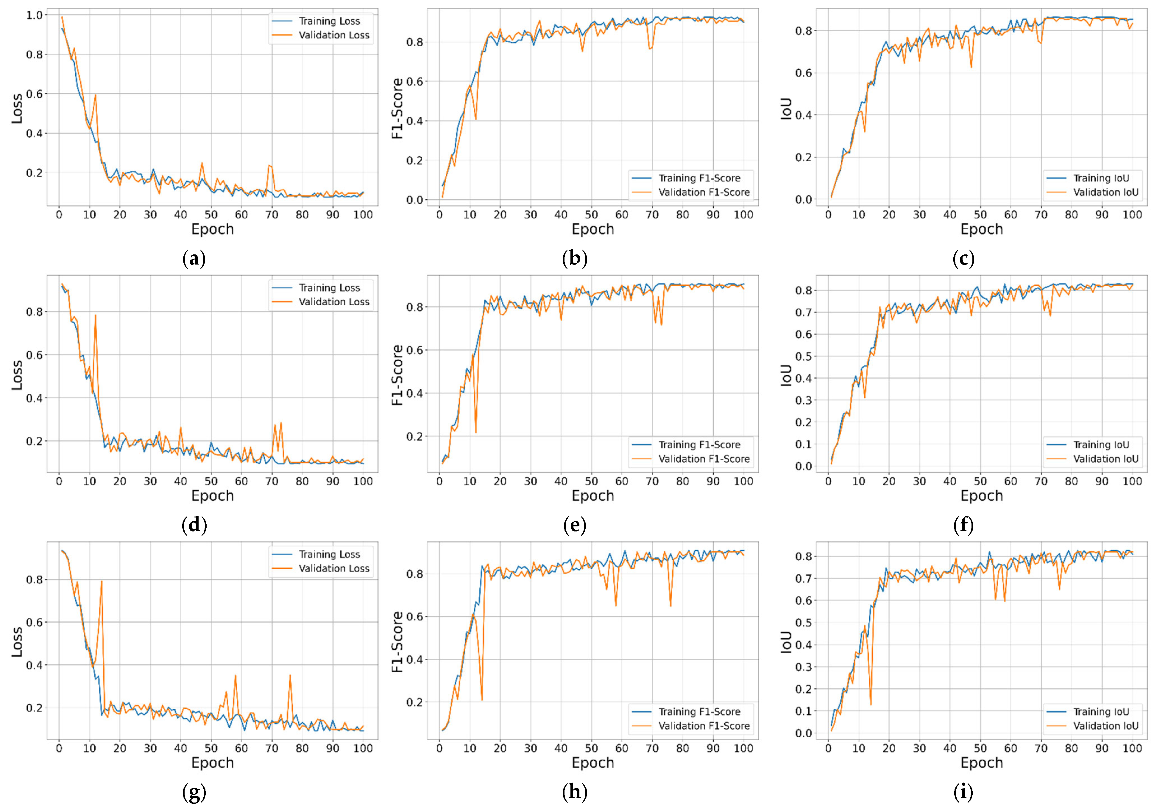
Figure A3 and Figure A4 visualize the training and validation loss, F1-Score and IoU progression across epochs for the trained U-Net and Attention U-Net models with softmax activation function, respectively.
Figure A3. Training and validation loss, F1-Score, and IoU per epoch results for the trained U-Net models with softmax output layer: (ac) U-Net with Dice Loss; (df) U-Net with Dice BCE Loss; (gi) U-Net with Focal Loss.
Ai 06 00212 g0a3
Figure A4. Training and validation loss, F1-Score, and IoU per epoch results for the trained Attention U-Net models with softmax output layer: (ac) Attention U-Net with Dice Loss; (df) Attention U-Net with Dice BCE Loss; (gi) Attention U-Net with Focal Loss.
Ai 06 00212 g0a4

Appendix B

This appendix provides a detailed evaluation of peak-localization accuracy for the two smoothing strategies investigated in Section 4.3.2. Table A1 lists, for every subject, the slice index of the WAO maximum obtained from the raw curves as well as after Gaussian and Butterworth filtering. Table A2 aggregates these data by counting the number of cases in which the smoothed peak lies exactly on, or one or two slices away from, the reference peak for both ground truth and predicted WAO curves. These summaries underpin the selection of the Gaussian filter.
Table A1. Per-patient slice index of the WAO peak. The table lists, for each of the 110 subjects, the peak obtained from the raw ground truth WAO curve, the peak after Gaussian and Butterworth smoothing of the ground truth curve, and the corresponding three peaks for the model-predicted WAO curve.
Patient IDGT PeakGT Gaussian PeakGT Butterworth PeakPredicted PeakPredicted Gaussian PeakPredicted Butterworth Peak
TCGA_DU_7010_19860307353536363536
TCGA_DU_8162_19961029111314121314
TCGA_FG_A4MT_20020212111114101716
TCGA_FG_5964_20010511131314121414
TCGA_DU_A5TS_19970726141314141415
TCGA_HT_7692_19960724151719151819
TCGA_DU_5849_19950405202224192224
TCGA_FG_A60K_20040224454445374345
TCGA_HT_7475_19970918172222182222
TCGA_FG_6691_20020405202424222424
TCGA_HT_7684_19950816141617141617
TCGA_CS_6188_20010812141516000
TCGA_HT_7694_199504049111161111
TCGA_DU_A5TR_19970726141617141617
TCGA_DU_7300_19910814141516141617
TCGA_DU_7018_19911220121818111518
TCGA_DU_7301_19911112192122172121
TCGA_DU_7302_19911203182122222222
TCGA_HT_8018_19970411888888
TCGA_FG_6692_20020606151718161717
TCGA_DU_5854_19951104252526252525
TCGA_DU_7299_1991041722232492425
TCGA_HT_A5RC_19990831242221192122
TCGA_HT_8105_19980826161921161921
TCGA_HT_8563_19981209101111101010
TCGA_HT_A61A_20000127223231455453
TCGA_CS_4944_20010208889899
TCGA_FG_7643_20021104272728242626
TCGA_DU_8163_19961119141516151515
TCGA_CS_6669_20020102101313111213
TCGA_DU_7013_19860523242322252323
TCGA_FG_8189_20030516182324182424
TCGA_HT_8111_19980330141615141615
TCGA_CS_5396_20010302131516141516
TCGA_DU_7294_19890104212324212324
TCGA_HT_7879_19981009101213121313
TCGA_EZ_7264_20010816161817161817
TCGA_DU_8164_19970111202525202425
TCGA_HT_7860_19960513141414141414
TCGA_HT_7881_19981015262729222629
TCGA_DU_6400_19830518202123152023
TCGA_HT_7686_19950629101111111111
TCGA_FG_6688_20020215192424242624
TCGA_DU_6401_19831001192729232729
TCGA_CS_4943_20000902151313151313
TCGA_DU_A5TW_19980228162021171818
TCGA_HT_7473_1997082614141691315
TCGA_DU_5853_19950823252728272727
TCGA_CS_6290_20000917788888
TCGA_DU_6399_19830416181820141820
TCGA_CS_4942_19970222101110101111
TCGA_DU_5872_19950223333741333841
TCGA_HT_7616_19940813161820141820
TCGA_DU_7019_19940908111415111414
TCGA_DU_5871_19941206192123172122
TCGA_CS_6666_20011109151717141617
TCGA_FG_7637_20000922191821162122
TCGA_CS_5397_20010315788688
TCGA_CS_4941_19960909111314111313
TCGA_HT_7874_199509028101091111
TCGA_DU_6404_19850629293335293335
TCGA_DU_8166_19970322202325182223
TCGA_HT_7605_19950916262524222525
TCGA_FG_5962_20000626252630223031
TCGA_HT_7856_19950831161720141720
TCGA_DU_6405_19851005414545434545
TCGA_DU_5852_19950709151515141313
TCGA_HT_8114_19981030111314111414
TCGA_FG_7634_20000128192122181919
TCGA_CS_6665_20010817161415131415
TCGA_HT_7855_1995102081111151111
TCGA_HT_7602_19951103888888
TCGA_DU_8167_19970402121617121618
TCGA_DU_7309_19960831242424122424
TCGA_DU_5874_19950510222323212323
TCGA_DU_6407_19860514202425212426
TCGA_HT_7690_19960312141616131616
TCGA_HT_7884_19980913688688
TCGA_DU_5855_19951217141617131617
TCGA_DU_7298_1991032410121281212
TCGA_FG_A4MU_20030903131416161617
TCGA_CS_6667_20011105101212111312
TCGA_HT_7877_19980917202222202222
TCGA_DU_A5TT_19980318414346414446
TCGA_FG_6689_20020326252828282828
TCGA_HT_A61B_19991127413939403936
TCGA_HT_8107_199807089101091010
TCGA_DU_A5TY_19970709222425222424
TCGA_HT_7608_19940304161617151616
TCGA_CS_6186_20000601151717141616
TCGA_DU_5851_19950428141617131617
TCGA_HT_7693_19950520111313131313
TCGA_DU_8165_19970205121313151515
TCGA_DU_8168_19970503192020181920
TCGA_DU_7008_19830723131822121922
TCGA_HT_7882_19970125111518171619
TCGA_DU_7304_19930325262523212023
TCGA_CS_5393_19990606588889
TCGA_DU_7014_19860618353535353534
TCGA_HT_8106_1997072714121371112
TCGA_CS_6668_20011025151717151717
TCGA_HT_7680_19970202557557
TCGA_FG_6690_20020226303030293030
TCGA_DU_6408_19860521272832272731
TCGA_DU_A5TU_19980312121415131415
TCGA_HT_A616_19991226131516151516
TCGA_CS_5395_19981004121212131211
TCGA_HT_8113_19930809141514111413
TCGA_DU_A5TP_19970614232527222426
TCGA_DU_7306_19930512161920152020
Table A2. Absolute deviation (in slices) between the filter-based peak location and its reference peak. Counts of subjects whose Gaussian or Butterworth smoothed peak lies exactly on, or one/two slices away from, the raw WAO peak, shown separately for ground truth and predicted curves. Totals indicate the number of subjects within ±2 slices.
Absolute Peak Difference ValueGaussian Filter—GTButterworth Filter—
GT
Gaussian Filter—PredictedButterworth Filter—Predicted
018122116
126182118
241232626
Total85536860

References

  1. Mazurowski, M.A.; Clark, K.; Czarnek, N.M.; Shamsesfandabadi, P.; Peters, K.B.; Saha, A. Radiogenomics of lower-grade glioma: Algorithmically-assessed tumor shape is associated with tumor genomic subtypes and patient outcomes in a multi-institutional study with The Cancer Genome Atlas data. J. Neurooncol. 2017, 133, 27–35. [Google Scholar] [CrossRef] [PubMed]
  2. Ostrom, Q.T.; Price, M.; Neff, C.; Cioffi, G.; Waite, K.A.; Kruchko, C.; Barnholtz-Sloan, J.S. CBTRUS Statistical Report: Primary Brain and Other Central Nervous System Tumors Diagnosed in the United States in 2016–2020. Neuro-Oncology 2023, 25, iv1–iv99. [Google Scholar] [CrossRef] [PubMed]
  3. Ullah, W.; Naveed, H.; Ali, S. Deep Learning for Precise MRI Segmentation of Lower-Grade Gliomas. Sustain. Mach. Intell. J. 2025, 10, 23–36. [Google Scholar] [CrossRef]
  4. Menze, B.H.; Jakab, A.; Bauer, S.; Kalpathy-Cramer, J.; Farahani, K.; Kirby, J.; Burren, Y.; Porz, N.; Slotboom, J.; Wiest, R.; et al. The Multimodal Brain Tumor Image Segmentation Benchmark (BRATS). IEEE Trans. Med. Imaging 2015, 34, 1993–2024. [Google Scholar] [CrossRef]
  5. Naser, M.A.; Deen, M.J. Brain tumor segmentation and grading of lower-grade glioma using deep learning in MRI images. Comput. Biol. Med. 2020, 121, 103758. [Google Scholar] [CrossRef]
  6. Bowden, S.G.; Neira, J.A.; Gill, B.J.A.; Ung, T.H.; Englander, Z.K.; Zanazzi, G.; Chang, P.D.; Samanamud, J.; Grinband, J.; Sheth, S.A.; et al. Sodium Fluorescein Facilitates Guided Sampling of Diagnostic Tumor Tissue in Nonenhancing Gliomas. Neurosurgery 2018, 82, 719. [Google Scholar] [CrossRef]
  7. Dhar, T.; Dey, N.; Borra, S.; Sherratt, R.S. Challenges of Deep Learning in Medical Image Analysis—Improving Explainability and Trust. IEEE Trans. Technol. Soc. 2023, 4, 68–75. [Google Scholar] [CrossRef]
  8. Castiglioni, I.; Rundo, L.; Codari, M.; Leo, G.D.; Salvatore, C.; Interlenghi, M.; Gallivanone, F.; Cozzi, A.; D’Amico, N.C.; Sardanelli, F. AI applications to medical images: From machine learning to deep learning. Phys. Medica Eur. J. Med. Phys. 2021, 83, 9–24. [Google Scholar] [CrossRef]
  9. Jiang, X.; Hu, Z.; Wang, S.; Zhang, Y. Deep Learning for Medical Image-Based Cancer Diagnosis. Cancers 2023, 15, 3608. [Google Scholar] [CrossRef]
  10. Litjens, G.; Kooi, T.; Bejnordi, B.E.; Setio, A.A.A.; Ciompi, F.; Ghafoorian, M.; van der Laak, J.A.W.M.; van Ginneken, B.; Sánchez, C.I. A survey on deep learning in medical image analysis. Med. Image Anal. 2017, 42, 60–88. [Google Scholar] [CrossRef]
  11. Yildirim, K.; Bozdag, P.G.; Talo, M.; Yildirim, O.; Karabatak, M.; Acharya, U.R. Deep learning model for automated kidney stone detection using coronal CT images. Comput. Biol. Med. 2021, 135, 104569. [Google Scholar] [CrossRef]
  12. Bhati, D.; Neha, F.; Amiruzzaman, M. A Survey on Explainable Artificial Intelligence (XAI) Techniques for Visualizing Deep Learning Models in Medical Imaging. J. Imaging 2024, 10, 239. [Google Scholar] [CrossRef]
  13. Vu, M.H.; Grimbergen, G.; Nyholm, T.; Löfstedt, T. Evaluation of multislice inputs to convolutional neural networks for medical image segmentation. Med. Phys. 2020, 47, 6216–6231. [Google Scholar] [CrossRef]
  14. Yu, Q.; Xia, Y.; Xie, L.; Fishman, E.K.; Yuille, A.L. Thickened 2D Networks for Efficient 3D Medical Image Segmentation. arXiv 2019, arXiv:1904.01150. [Google Scholar] [CrossRef]
  15. Milletari, F.; Navab, N.; Ahmadi, S.-A. V-Net: Fully Convolutional Neural Networks for Volumetric Medical Image Segmentation. In Proceedings of the 2016 Fourth International Conference on 3D Vision (3DV), Stanford, CA, USA, 25–28 October 2016; pp. 565–571. [Google Scholar] [CrossRef]
  16. Çiçek, Ö.; Abdulkadir, A.; Lienkamp, S.S.; Brox, T.; Ronneberger, O. 3D U-Net: Learning Dense Volumetric Segmentation from Sparse Annotation. In Proceedings of the Medical Image Computing and Computer-Assisted Intervention—MICCAI 2016, Athens, Greece, 17–21 October 2016; Ourselin, S., Joskowicz, L., Sabuncu, M.R., Unal, G., Wells, W., Eds.; Springer International Publishing: Cham, Switzerland, 2016; pp. 424–432. [Google Scholar] [CrossRef]
  17. Zhang, Y.; Liao, Q.; Ding, L.; Zhang, J. Bridging 2D and 3D segmentation networks for computation-efficient volumetric medical image segmentation: An empirical study of 2.5D solutions. Comput. Med. Imaging Graph. 2022, 99, 102088. [Google Scholar] [CrossRef] [PubMed]
  18. Fawzi, A.; Achuthan, A.; Belaton, B. Brain Image Segmentation in Recent Years: A Narrative Review. Brain Sci. 2021, 11, 1055. [Google Scholar] [CrossRef] [PubMed]
  19. Shen, D.; Wu, G.; Suk, H.-I. Deep Learning in Medical Image Analysis. Annu. Rev. Biomed. Eng. 2017, 19, 221–248. [Google Scholar] [CrossRef]
  20. Voulodimos, A.; Doulamis, N.; Doulamis, A.; Protopapadakis, E. Deep Learning for Computer Vision: A Brief Review. Comput. Intell. Neurosci. 2018, 2018, 7068349. [Google Scholar] [CrossRef]
  21. Pasvantis, K.; Protopapadakis, E. Enhancing Deep Learning Model Explainability in Brain Tumor Datasets Using Post-Heuristic Approaches. J. Imaging 2024, 10, 232. [Google Scholar] [CrossRef]
  22. Ronneberger, O.; Fischer, P.; Brox, T. U-Net: Convolutional Networks for Biomedical Image Segmentation. In Proceedings of the Medical Image Computing and Computer-Assisted Intervention—MICCAI 2015, Munich, Germany, 5–9 October 2015; Navab, N., Hornegger, J., Wells, W.M., Frangi, A.F., Eds.; Springer International Publishing: Cham, Switzerland, 2015; pp. 234–241. [Google Scholar] [CrossRef]
  23. Azad, R.; Aghdam, E.K.; Rauland, A.; Jia, Y.; Avval, A.H.; Bozorgpour, A.; Karimijafarbigloo, S.; Cohen, J.P.; Adeli, E.; Merhof, D. Medical Image Segmentation Review: The success of U-Net 2022. IEEE Trans. Pattern Anal. Mach. Intell. 2024, 46, 10076–10095. [Google Scholar] [CrossRef]
  24. Mazurowski, M.A.; Buda, M.; Saha, A.; Bashir, M.R. Deep learning in radiology: An overview of the concepts and a survey of the state of the art with focus on MRI. J. Magn. Reson. Imaging 2019, 49, 939–954. [Google Scholar] [CrossRef] [PubMed]
  25. Voulodimos, A.; Protopapadakis, E.; Katsamenis, I.; Doulamis, A.; Doulamis, N. A Few-Shot U-Net Deep Learning Model for COVID-19 Infected Area Segmentation in CT Images. Sensors 2021, 21, 2215. [Google Scholar] [CrossRef] [PubMed]
  26. Maganaris, C.; Protopapadakis, E.; Bakalos, N.; Doulamis, N.; Kalogeras, D.; Angeli, A. Evaluating Transferability for Covid 3D Localization Using CT SARS-CoV-2 segmentation models 2022. arXiv 2022, arXiv:2205.02152. [Google Scholar] [CrossRef]
  27. Qin, C.; Wu, Y.; Zeng, J.; Tian, L.; Zhai, Y.; Li, F.; Zhang, X. Joint Transformer and Multi-scale CNN for DCE-MRI Breast Cancer Segmentation. Soft Comput. 2022, 26, 8317–8334. [Google Scholar] [CrossRef]
  28. Özkaraca, O.; Bağrıaçık, O.İ.; Gürüler, H.; Khan, F.; Hussain, J.; Khan, J.; Laila, U. e Multiple Brain Tumor Classification with Dense CNN Architecture Using Brain MRI Images. Life 2023, 13, 349. [Google Scholar] [CrossRef]
  29. Wong, K.C.L.; Moradi, M.; Wu, J.; Syeda-Mahmood, T. Identifying disease-free chest x-ray images with deep transfer learning. In Proceedings of the Medical Imaging 2019: Computer-Aided Diagnosis, San Diego, CA, USA, 17–20 February 2019; SPIE: Bellingham, WA, USA, 2019; Volume 10950, pp. 179–184. [Google Scholar] [CrossRef]
  30. Muhammad Hussain, N.; Rehman, A.U.; Othman, M.T.B.; Zafar, J.; Zafar, H.; Hamam, H. Accessing Artificial Intelligence for Fetus Health Status Using Hybrid Deep Learning Algorithm (AlexNet-SVM) on Cardiotocographic Data. Sensors 2022, 22, 5103. [Google Scholar] [CrossRef]
  31. Dorfner, F.J.; Patel, J.B.; Kalpathy-Cramer, J.; Gerstner, E.R.; Bridge, C.P. A review of deep learning for brain tumor analysis in MRI. Npj Precis. Oncol. 2025, 9, 2. [Google Scholar] [CrossRef]
  32. Pravitasari, A.A.; Iriawan, N.; Almuhayar, M.; Azmi, T.; Irhamah, I.; Fithriasari, K.; Purnami, S.W.; Ferriastuti, W. UNet-VGG16 with transfer learning for MRI-based brain tumor segmentation. TELKOMNIKA Telecommun. Comput. Electron. Control 2020, 18, 1310–1318. [Google Scholar] [CrossRef]
  33. Bukhari, S.T.; Mohy-ud-Din, H. E1D3 U-Net for Brain Tumor Segmentation: Submission to the RSNA-ASNR-MICCAI BraTS 2021 Challenge 2022. arXiv 2022, arXiv:2110.02519. [Google Scholar] [CrossRef]
  34. Allah, A.M.G.; Sarhan, A.M.; Elshennawy, N.M. Edge U-Net: Brain tumor segmentation using MRI based on deep U-Net model with boundary information. Expert Syst. Appl. 2023, 213, 118833. [Google Scholar] [CrossRef]
  35. Kamnitsas, K.; Ledig, C.; Newcombe, V.F.J.; Simpson, J.P.; Kane, A.D.; Menon, D.K.; Rueckert, D.; Glocker, B. Efficient multi-scale 3D CNN with fully connected CRF for accurate brain lesion segmentation. Med. Image Anal. 2017, 36, 61–78. [Google Scholar] [CrossRef]
  36. Pham, T.X.; Siarry, P.; Oulhadj, H. Integrating fuzzy entropy clustering with an improved PSO for MRI brain image segmentation. Appl. Soft Comput. 2018, 65, 230–242. [Google Scholar] [CrossRef]
  37. Pham, T.X.; Siarry, P.; Oulhadj, H. A multi-objective optimization approach for brain MRI segmentation using fuzzy entropy clustering and region-based active contour methods. Magn. Reson. Imaging 2019, 61, 41–65. [Google Scholar] [CrossRef] [PubMed]
  38. Wang, G.; Li, W.; Ourselin, S.; Vercauteren, T. Automatic Brain Tumor Segmentation Using Convolutional Neural Networks with Test-Time Augmentation. In Brainlesion: Glioma, Multiple Sclerosis, Stroke and Traumatic Brain Injuries; Crimi, A., Bakas, S., Kuijf, H., Keyvan, F., Reyes, M., van Walsum, T., Eds.; Springer International Publishing: Cham, Switzerland, 2019; pp. 61–72. [Google Scholar] [CrossRef]
  39. Chen, C.; Qin, C.; Qiu, H.; Tarroni, G.; Duan, J.; Bai, W.; Rueckert, D. Deep Learning for Cardiac Image Segmentation: A Review. Front. Cardiovasc. Med. 2020, 7, 25. [Google Scholar] [CrossRef] [PubMed]
  40. Sudre, C.H.; Li, W.; Vercauteren, T.; Ourselin, S.; Jorge Cardoso, M. Generalised Dice Overlap as a Deep Learning Loss Function for Highly Unbalanced Segmentations. In Deep Learning in Medical Image Analysis and Multimodal Learning for Clinical Decision Support; Cardoso, M.J., Arbel, T., Carneiro, G., Syeda-Mahmood, T., Tavares, J.M.R.S., Moradi, M., Bradley, A., Greenspan, H., Papa, J.P., Madabhushi, A., Eds.; Springer International Publishing: Cham, Switzerland, 2017; pp. 240–248. [Google Scholar] [CrossRef]
  41. Yu, L.; Cheng, J.-Z.; Dou, Q.; Yang, X.; Chen, H.; Qin, J.; Heng, P.-A. Automatic 3D Cardiovascular MR Segmentation with Densely-Connected Volumetric ConvNets. In Medical Image Computing and Computer-Assisted Intervention—MICCAI 2017; Descoteaux, M., Maier-Hein, L., Franz, A., Jannin, P., Collins, D.L., Duchesne, S., Eds.; Springer International Publishing: Cham, Switzerland, 2017; pp. 287–295. [Google Scholar] [CrossRef]
  42. Xia, Q.; Yao, Y.; Hu, Z.; Hao, A. Automatic 3D Atrial Segmentation from GE-MRIs Using Volumetric Fully Convolutional Networks. In Statistical Atlases and Computational Models of the Heart; Atrial Segmentation and LV Quantification Challenges; Pop, M., Sermesant, M., Zhao, J., Li, S., McLeod, K., Young, A., Rhode, K., Mansi, T., Eds.; Springer International Publishing: Cham, Switzerland, 2019; pp. 211–220. [Google Scholar] [CrossRef]
  43. Tejani, A.S.; Klontzas, M.E.; Gatti, A.A.; Mongan, J.T.; Moy, L.; Park, S.H.; Kahn, C.E. Checklist for Artificial Intelligence in Medical Imaging (CLAIM): 2024 Update. Radiol. Artif. Intell. 2024, 6, e240300. [Google Scholar] [CrossRef] [PubMed]
  44. FDA. FDA Good Machine Learning Practice for Medical Device Development: Guiding Principles. Available online: https://www.fda.gov/medical-devices/software-medical-device-samd/good-machine-learning-practice-medical-device-development-guiding-principles (accessed on 26 August 2025).
  45. Brain MRI Segmentation. Available online: https://www.kaggle.com/datasets/mateuszbuda/lgg-mri-segmentation (accessed on 9 July 2024).
  46. TCGA-LGG Phenotype Research Group—The Cancer Imaging Archive (TCIA) Public Access—Cancer Imaging Archive Wiki. Available online: https://wiki.cancerimagingarchive.net/display/Public/TCGA-LGG+Phenotype+Research+Group (accessed on 9 July 2024).
  47. The Cancer Imaging Archive, TCGA-LGG. Available online: https://www.cancerimagingarchive.net/collection/tcga-lgg/#citations (accessed on 9 July 2024).
  48. Paszke, A.; Gross, S.; Massa, F.; Lerer, A.; Bradbury, J.; Chanan, G.; Killeen, T.; Lin, Z.; Gimelshein, N.; Antiga, L.; et al. PyTorch: An imperative style, high-performance deep learning library. In Proceedings of the 33rd International Conference on Neural Information Processing Systems, Vancouver, BC, Canada, 3 December 2019; Curran Associates Inc.: Red Hook, NY, USA, 2019; pp. 8026–8037. [Google Scholar]
  49. Oktay, O.; Schlemper, J.; Folgoc, L.L.; Lee, M.; Heinrich, M.; Misawa, K.; Rueckert, D. Attention U-Net: Learning Where to Look for the Pancreas. arXiv 2018, arXiv:1804.03999. [Google Scholar] [CrossRef]
  50. Kingma, D.P.; Ba, J. Adam: A Method for Stochastic Optimization. arXiv 2014, arXiv:1412.6980. [Google Scholar] [CrossRef]
  51. Ruder, S. An overview of gradient descent optimization algorithms. arXiv 2017, arXiv:1609.04747. [Google Scholar] [CrossRef]
  52. Abraham, N.; Khan, N.M. A Novel Focal Tversky loss function with improved Attention U-Net for lesion segmentation. arXiv 2018, arXiv:1810.07842. [Google Scholar] [CrossRef]
  53. Vossough, A.; Khalili, N.; Familiar, A.M.; Gandhi, D.; Viswanathan, K.; Tu, W.; Haldar, D.; Bagheri, S.; Anderson, H.; Haldar, S.; et al. Training and Comparison of nnU-Net and DeepMedic Methods for Autosegmentation of Pediatric Brain Tumors. AJNR Am. J. Neuroradiol. 2024, 45, 1081–1089. [Google Scholar] [CrossRef]
  54. Matta, S.; Lamard, M.; Zhang, P.; Le Guilcher, A.; Borderie, L.; Cochener, B.; Quellec, G. A systematic review of generalization research in medical image classification. Comput. Biol. Med. 2024, 183, 109256. [Google Scholar] [CrossRef]
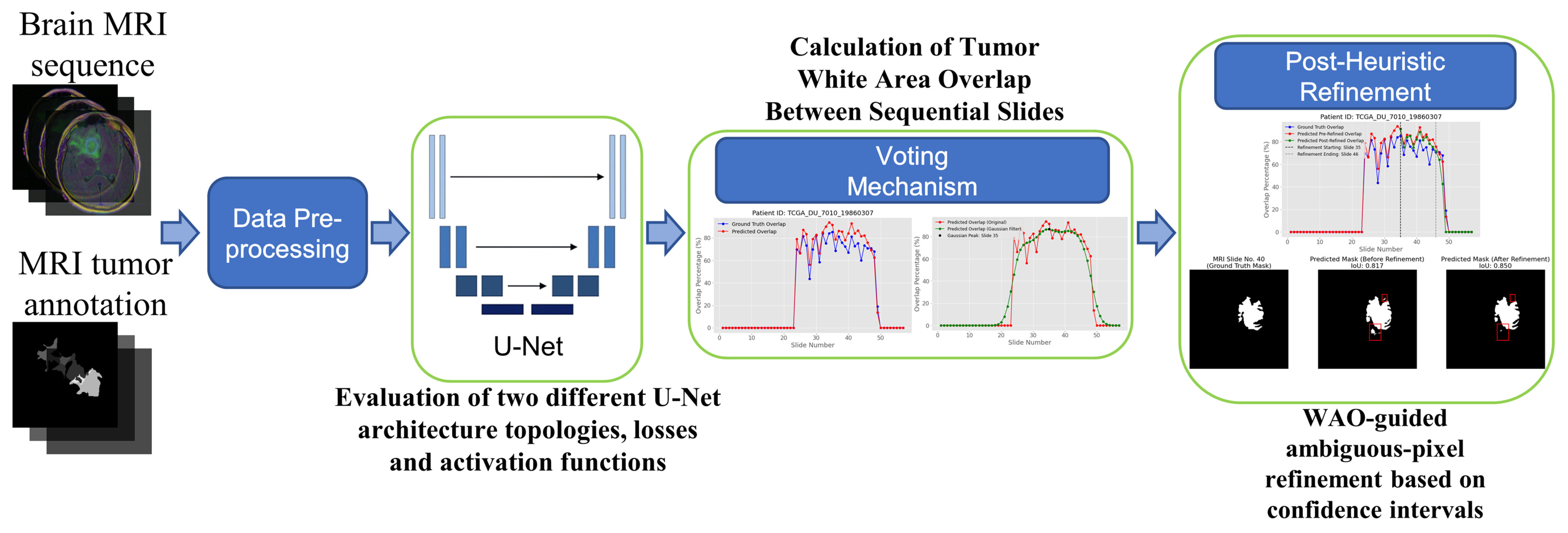
Figure 1. Graphical abstract of the proposed methodology.
Ai 06 00212 g001
Figure 2. Diagnosis distribution across the 3929 FLAIR slices in the TCGA-LGG dataset. Bars report the absolute number of images labelled tumor (positive mask) and Normal (empty mask).
Ai 06 00212 g002
Figure 3. MRI slice-level examples from patient with ID “TCGA_CS_4941_19960909”. (a,d) Raw FLAIR images; (b,e) ground truth binary expert masks; (c,f) image–mask (red) overlays.
Ai 06 00212 g003
Figure 4. Anatomical order visualization for patient with ID “TCGA_CS_4941_19960909”: (a) Complete set of 23 axial FLAIR slices; (b) ground truth tumor masks.
Ai 06 00212 g004
Figure 5. Image–mask (red) overlays for all 23 slices for patient with ID “TCGA_CS_4941_19960909”.
Ai 06 00212 g005
Figure 6. Schematic representation of the defined U-Net architectures.
Ai 06 00212 g006
Figure 7. Schematic representation of the defined Attention U-Net architectures.
Ai 06 00212 g007
Figure 8. Performance metrics per architecture with sigmoid, per loss: (a) Accuracy; (b) Precision; (c) Recall; (d) F1-Score; (e) IoU; (f) AUC.
Ai 06 00212 g008
Figure 9. Training and validation loss, IoU, and F1-Score per epoch results for the best performing trained Attention U-Net model with sigmoid output layer: (a) Loss; (b) IoU; (c) F1-Score.
Ai 06 00212 g009
Figure 10. Performance metrics per architecture with softmax, per loss: (a) Accuracy; (b) Precision; (c) Recall; (d) F1-Score; (e) IoU; (f) AUC.
Ai 06 00212 g010
Figure 11. Training and validation loss, IoU, and F1-Score per epoch results for the best performing trained Attention U-Net model with softmax output layer: (a) Loss; (b) IoU; (c) F1-Score.
Ai 06 00212 g011
Figure 12. Visual comparison of three difficult cases for the best-performing models with different output activation function layers. Each row showcases the results for the same patient case. Each subfigure showcases ground truth segmentation mask, predicted segmentation mask, and original image overlaid with the predicted segmentation output mask (red): (a,c,e) Attention U-Net paired with DiceBCE with sigmoid output; (b,d,f) Attention U-Net paired with DiceBCE with softmax output. Per-slice IoU, precision, recall and F1-score are reported beneath each overlay.
Ai 06 00212 g012
Figure 13. Qualitative evaluation with examples in which the Attention U-Net and DiceBCE with softmax head predicts accurate tumor segmentation masks (IoU > 0.89). Each subfigure displays the original image, the ground truth segmentation mask, the predicted segmentation mask, and the original image overlaid with the predicted segmentation output mask (red) generated by the top-performing segmentation model: (a) showcases an example of a segmentation output of 0.945 IoU; (b) showcases an example of a segmentation output of 0.939 IoU; (c) showcases an example of a segmentation output of 0.892 IoU.
Ai 06 00212 g013
Figure 14. Qualitative evaluation with examples in which the Attention U-Net and DiceBCE with softmax head predicts suboptimal and irregular tumor segmentation masks (IoU < 0.60). Each subfigure displays the original image, the ground truth segmentation mask, the predicted segmentation mask, and the original image overlaid with the predicted segmentation output mask (red) generated by the top-performing segmentation model: (a) showcases an example of a segmentation output of 0.599 IoU; (b) showcases an example of a segmentation output of 0.598 IoU; (c) showcases an example of a segmentation output of 0.378 IoU.
Ai 06 00212 g014
Figure 15. White area overlap percentage between sequential slides for patient with ID “TCGA_DU_7010_19860307”. The blue curve represents the white overlapping white pixels of the ground truth masks, and the red curve the predicted white overlapping pixels.
Ai 06 00212 g015
Figure 16. Ground truth and predicted overlap curve peak points identification for patient with ID “TCGA_DU_7010_19860307”: (a) ground truth with Gaussian Filter peak identification; (b) ground truth with Butterworth Filter peak identification; (c) predicted with Gaussian Filter peak identification; (d) predicted with Butterworth Filter peak identification. The blue curves represent the white overlapping white pixels of the ground truth masks, the red curves the predicted white overlapping pixels, while the green lines represent the smoothed ground truth and predicted overlap using each peak localization method.
Ai 06 00212 g016
Figure 17. Inter-slice WAO percentage after removing 1.5% of the most ambiguous pixels for patient with ID “TCGA_DU_7010_19860307”. The blue curve represents the white overlapping pixels of the ground truth masks, the red curve the predicted white overlapping pixels, while the green curve represents the refined predicted overlap by removing the ambiguous pixels with a 1.5% threshold.
Ai 06 00212 g017
Figure 18. Qualitative evaluation of the refinement strategy by removing the ambiguous pixels with a 1.5% threshold on patient with ID “TCGA_DU_7010_19860307”. (aq) Each triplet (left to right) displays the ground truth mask, the raw predicted mask, and the refined predicted mask for the top-performing segmentation model for MRI slices 35 to 51.
Ai 06 00212 g018aAi 06 00212 g018b
Figure 19. Inter-slice WAO percentage with early-stop window (MRI slides 35 to 46) after removing 1.5% of the most ambiguous pixels for patient with ID “TCGA_DU_7010_19860307”. The blue curve represents the white overlapping pixels of the ground truth masks, the red curve the predicted white overlapping pixels, while the green curve represents the refined predicted overlap by removing the ambiguous pixels with a 1.5% threshold.
Ai 06 00212 g019
Figure 20. Refined overlap percentage between sequential slides by adding ambiguous pixels for patient with ID “TCGA_DU_5872_19950223”: (a) adding ambiguous pixels with a 1.5% threshold; (b) adding ambiguous pixels with 0.3% threshold; (c) combining the 0.3% adding threshold with the computed refinement window (MRI slixes 38 to 49). The blue curve represents the white overlapping pixels of the ground truth masks, the red curve the predicted white overlapping pixels, while the green curve represents the refined predicted overlap.
Ai 06 00212 g020
Figure 21. Qualitative evaluation of the refinement strategy by adding ambiguous pixels on patient with ID “TCGA_DU_5872_19950223”: (a,c) with a 1.5% threshold percentage and computed refinement window; (b,d) with a 0.3% threshold percentage and computed refinement window. Each triplet (left to right) displays the ground truth mask, the raw predicted mask, and the refined predicted mask for the top-performing segmentation model.
Ai 06 00212 g021
Figure 22. Sample outcomes of the heuristic refinement rules. (a,b) Patient with ID “TCGA_DU_7010_19860307” at 1.5% threshold: (a) removal of ambiguous pixels improves IoU from 0.702 to 0.755; (b) addition at the same threshold reduces IoU to 0.626. (c,d) Patient with ID “TCGA_DU_5872_19950223” at 0.3% threshold: (c) removal lowers IoU from 0.886 to 0.874; (d) addition increases IoU from 0.886 to 0.894. Each triplet (left to right) displays the ground truth mask, the raw predicted mask, and the refined predicted mask for the top-performing segmentation model.
Ai 06 00212 g022
Table 1. Summary of related work in AI studies in medical imaging.
Reference IDType/ArchitectureMetricsLimitations
[21]Post-Processing Mechanisms
LIME Library/image explainer
ResNet50V2
Accuracy,
Precision,
Recall,
F1-Score
Reliant on initial segmentation quality
[22]Segmentation
U-Net
IoU,
Dice
Heavy data augmentation,
Can lead to slice-wise inconsistencies
[25]Segmentation
Few-Shot U-Net
Accuracy,
Precision,
Recall,
F1-Score,
IoU
Data dependency
[26]Transfer learning
3D COVID-19 CT segmentation
Accuracy,
Precision,
Recall,
F1-Score
Domain shift,
Limited data,
Limited zero-shot transfer
[27]Segmentation
U-Net
Dice,
IoU,
Sensitivity,
Positive Predicted Value
Further study with 3D segmentation needed
[28]Classification
DenseNet
AccuracyHigh computational cost and inference time
[29]Classification
Inception-ResNet-v2
Precision,
Recall
Trade-off between recall and precision
[30]Classification
Hybrid AlexNet–SVM
Accuracy,
Precision,
Recall
Computational complexity
[32]Segmentation
UNet-VGG16
Accuracy,
Dice
Optimal epoch not decided for optimal computing time
[33]Segmentation
E1D3 U-Net
Dice,
Hausdorff Distance
Generalization to raw clinical MRI or other tumor types is not proven
[34]Segmentation
Edge U-Net
IoU,
Dice
Precomputed edge maps
[35]Segmentation
3D CNN and CRF
DiceCRF tuning,
Higher compute
[36]Segmentation
Fuzzy Clustering and PSO
Dice,
Accuracy
Parameter-sensitive
[37]Segmentation
Fuzzy Clustering and Active Contour
Dice,
Hausdorff Distance,
Jaccard Index,
Accuracy
Limited scalability
Table 2. Class distribution obtained with a slice-stratified 70%:20%:10% split. Slices from a single patient may be present in more than one subset, but the tumor/normal ratio is preserved by stratification on the diagnosis label.
SetClassLabelsSamples CountProportion
TrainTumor961275069.99%
Normal1789
ValTumor28882521.00%
Normal537
TestTumor1243549.01%
Normal230
Table 3. Patient-oriented datasets split class distribution statistics. Class distribution for the patient-oriented 70%:20%:10% split. All slices belonging to a patient remain in the same subset, preventing cross-patient leakage and providing a stricter test of model generalization.
SetPatientsClassLabelsSamples CountProportion
Train79Tumor991282871.98%
Normal1837
Val20Tumor25670818.02%
Normal452
Test11Tumor12639310.00%
Normal267
Table 4. Overall performance of DL segmentation models with sigmoid activation function as output layer.
ArchitectureLossAccuracyPrecisionRecallF1-ScoreIoUAUCEpoch
U-NetDice0.99780.91820.88030.89740.81660.947397
U-NetDiceBCE0.97540.91030.89330.90060.82140.975371
U-NetFocal0.97320.87770.92480.89890.81940.968894
Attention U-Net 1Dice0.99810.91950.89680.90710.83190.953671
Attention U-Net 2Dice0.97040.85760.89050.87390.77390.934179
Attention U-NetDiceBCE0.99790.89970.90710.90210.82390.977877
Attention U-NetFocal0.95680.89330.90800.89880.81870.961497
1 Bold row indicates the best performing model with sigmoid activation function as output layer, using the second approach dataset split, where all slices from a single patient strictly belong to only one subset.2 Underlined row indicates the metrics obtained when coupling the same architecture and loss function that resulted in the best performing model, but using the first approach dataset split, where slices from a single patient may be present in more than one subset.
Table 5. Overall performance of DL segmentation models with softmax activation function as output layer.
ArchitectureLossAccuracyPrecisionRecallF1-ScoreIoUAUCEpoch
U-NetDice0.99270.88530.88630.88580.81870.951882
U-NetDiceBCE0.97460.89560.90780.90170.83480.963670
U-NetFocal0.97410.89850.91660.90750.81730.974396
Attention U-Net 3Dice0.99780.92010.91870.91940.85730.967476
Attention U-Net 4Dice0.97310.84280.90020.87040.76920.941270
Attention U-NetDiceBCE0.98150.90030.89990.90010.82270.974474
Attention U-NetFocal0.97560.89170.90720.89940.82010.961197
3 Bold row indicates the best performing model with softmax activation function as output layer, using the second approach dataset split, where all slices from a single patient strictly belong to only one subset.4 Underlined row indicates the metrics obtained when coupling the same architecture and loss function that resulted in the best performing model, but using the first approach dataset split, where slices from a single patient may be present in more than one subset.
Table 6. Summary of qualitative findings. Each row highlights a representative case and the corresponding observation.
Case TypeFigure ReferenceObservationRepresentative IoU Values
Softmax vs SigmoidFigure 12Softmax detects small lesions missed by sigmoid; prevents false positives in tumor-free slices0.615 vs. 0.000;
0.779 vs. 0.505
Accurate
segmentation
Figure 13Predicted masks closely follow tumor boundaries and details0.946, 0.940, 0.892
Inaccurate
segmentation
Figure 14Fragmented or under-segmented predictions, especially for complex tumor morphologies0.599, 0.598, 0.378
Table 7. Mean IoU (mIoU) for patient with ID “TCGA_DU_7010_19860307” at three stages: baseline, naïve 1.5% ambiguous-pixel removal applied to every slice (Raw Refinement), and the same removal restricted to the optimal window (slices 35–46).
mIoU
Before Refinement
mIoU
After Raw
Refinement
mIoU
After Refinement
with Ending
0.7990.7610.812
Table 8. Mean IoU (mIoU) for patient with ID “TCGA_DU_5872_19950223” under different ambiguous pixel addition settings: baseline, 1.5% ambiguous-pixel addition applied to every slice, 0.3% ambiguous-pixel addition applied to every slice, and the same 0.3% addition restricted to the optimal window (slices 38–49).
mIoU
Before Refinement
mIoU
After Raw
Refinement (1.5%)
mIoU
After Raw
Refinement (0.3%)
mIoU
After Refinement with Ending (0.3%)
0.9140.3550.4110.956
Table 9. Impact of ambiguous-pixel removal and addition on segmentation performance. For each threshold percentage, the table lists the cohort-wide mIoU before refinement, mIoU after refinement (averaged over the patients), and the number of patients whose individual IoU increased. Numbers in parenthesis indicate the ranking according to the mIoU score (higher value corresponds to better detection).
Refinement StrategymIoU
Before
Refinement
Threshold PercentagemIoU
After
Refinement
Number of Improved Patients
Ambiguous Removal0.8153%0.6109
2.5%0.64710
2%0.68712
1.5%0.72718
1%0.76925
0.5%0.80338
0.3%0.816 (3)56
0.2%0.825 (2)61
0.1%0.832 (1)67
Ambiguous Addition0.8153%0.5867
2.5%0.6229
2%0.6609
1.5%0.70210
1%0.74511
0.5%0.78419
0.3%0.79526
0.2%0.80028
0.1%0.80432
Disclaimer/Publisher’s Note: The statements, opinions and data contained in all publications are solely those of the individual author(s) and contributor(s) and not of MDPI and/or the editor(s). MDPI and/or the editor(s) disclaim responsibility for any injury to people or property resulting from any ideas, methods, instructions or products referred to in the content.