Complete Workflow for ER-IHC Pathology Database Revalidation

Abstract

Computer-aided systems can assist doctors in detecting cancer at an early stage using medical image analysis. In estrogen receptor immunohistochemistry (ER-IHC)-stained whole-slide images, automated cell identification and segmentation are helpful in the prediction scoring of hormone receptor status, which aids pathologists in determining whether to recommend hormonal therapy or other therapies for a patient. Accurate scoring can be achieved with accurate segmentation and classification of the nuclei. This paper presents two main objectives: first is to identify the top three models for this classification task and establish an ensemble model, all using 10-fold cross-validation strategy; second is to detect recurring misclassifications within the dataset to identify “misclassified nuclei” or “incorrectly labeled nuclei” for the nuclei class ground truth. The classification task is carried out using 32 pre-trained deep learning models from Keras Applications, focusing on their effectiveness in classifying negative, weak, moderate, and strong nuclei in the ER-IHC histopathology images. An ensemble learning with logistic regression approach is employed for the three best models. The analysis reveals that the top three performing models are EfficientNetB0, EfficientNetV2B2, and EfficientNetB4 with an accuracy of 94.37%, 94.36%, and 94.29%, respectively, and the ensemble model’s accuracy is 95%. We also developed a web-based platform for the pathologists to rectify the “faulty-class” nuclei in the dataset. The complete flow of this work can benefit the field of medical image analysis especially when dealing with intra-observer variability with a large number of images for ground truth validation.

1. Introduction

With more than 2.8 million new cases diagnosed annually, breast cancer is the most common malignancy among women [1] and remains a significant global public health concern. In 2020, it accounted for 8,418 new diagnoses (32.9%) out of 25,587 total cancer cases in women. Global estimates of age-standardized incidence and mortality rates were 49.3 and 20.7 per 100,000 women, respectively [2]. Clinically, breast cancer is categorized into distinct stages: Stage 0 is noninvasive but may progress to invasive disease; Stages I, IIa, and IIb represent early invasive stages; Stages IIIa, IIIb, and IIIc are considered locally advanced; and Stage IV corresponds to metastatic disease [2]. More than one hundred forms of cancer have been identified in medical science [3]. Among these, breast cancer has received substantial scientific attention and is one of the most extensively studied conditions in women’s health [4,5,6]. It is also the most frequently diagnosed cancer in women across 140 of 184 countries worldwide [7]. Furthermore, approximately 20% of breast cancer cases are attributable to modifiable lifestyle factors, including alcohol consumption, excess body weight, and physical inactivity [8].

When a patient is suspected of breast cancer, a biopsy procedure is performed to extract a breast tissue sample. Examples of biopsies are core needle, surgical, and lymph node to extract tumor tissues. Staining techniques are widely employed in tissue examination, with immunohistochemistry (IHC) and haematoxylin and eosin (H&E) being the most commonly used methods. Typically, H&E staining produces slides with contrasting blue-purple and pinkish-red tones, corresponding to haematoxylin and eosin, respectively. This technique is particularly useful for highlighting tissue morphology, structural organization, and cellular architecture. In contrast, IHC staining is extensively applied in breast cancer diagnosis, generating slides with blue and brown coloration, where the nuclei exhibit specific reactions in the presence of estrogen, progesterone, or ERBB2 receptor expression. H&E staining reveals tissue structure and cellular abnormalities, aiding in the understanding of disease behavior and morphology for prognosis. IHC detects specific proteins, guiding treatment decisions by identifying disease markers, subtypes, and treatment responses. Together, they provide a comprehensive view, combining morphological and molecular information for a more precise prognosis and tailored treatments.

In the biomedical industry, the review and diagnosis of breast cancer histopathology images by subject matter specialists is a delicate and time-consuming procedure. It is possible to help the diagnosing procedure by using technical instruments and software. Thus, costs and diagnostic time can be greatly reduced. Numerous studies using computational methods have been carried out for this goal. An artificial intelligence (AI)-based system was introduced in 2022 to support pathologists in their workflow, assisting with tasks such as distinguishing between cell types, assigning scores, and generating diagnoses [9]. Recent advances in deep learning have addressed the limitations of conventional computer vision, where manually designed algorithms often struggled to capture complex visual patterns. Unlike traditional approaches, deep neural networks can autonomously learn intricate image features directly from data, achieving performance comparable to expert pathologists. Although the development of deep learning models requires large datasets and substantial computational resources, the rapid growth in processing capabilities—particularly through the use of graphics processing units (GPUs)—has made effective training feasible. These advancements enable pathologists to dedicate less time to labor-intensive slide inspection and focus more on critical activities such as clinical decision-making and collaboration. Furthermore, portable devices such as tablets now facilitate automated analysis and remote specimen review at any time. For instance, in the substantia nigra of the mouse brain, the Aiforia deep learning platform was able to detect and count dopaminergic neurons within five seconds, a task that typically requires approximately forty-five minutes when performed manually [9].

Along with sophisticated algorithms and computer-assisted diagnostic methods, the introduction of digital slides into pathology practice has increased analytical capacities beyond the bounds of traditional microscopy, allowing for a more thorough application of medical knowledge [7]. Artificial intelligence (AI) now facilitates the identification of distinctive imaging biomarkers linked to disease mechanisms, thereby enhancing early diagnosis, improving prognostic assessment, and guiding the selection of optimal therapeutic strategies. These advancements enable pathologists to manage larger patient cohorts while preserving both diagnostic precision and prognostic accuracy. This integration is particularly significant given the increasing proportion of elderly patients and the fact that fewer than 2% of medical graduates pursue careers in pathology. The adoption of digital technologies in information management, data integration, and case review processes plays a vital role in addressing these challenges [8].

Breast cancer diagnosis and treatment have significantly benefited from the advancements in deep learning and computational techniques, particularly in the analysis of histopathology images. These techniques offer more accurate and efficient approaches, especially on exhaustive laborious tasks such as cell quantification. In computational analysis, to quantify the cells in tissue sample, the cells need to be segmented out from the tissue, and then classified into their respective class. The validated ground truth is essential to obtain an accurate classification model.

One notable contribution on classification comes from Alzubaidi et al. [10], who proposed a transfer learning method that exploits large sets of unlabeled medical images to improve the classification of skin and breast cancer. Their approach achieved a higher F1-score compared to traditional training methods, highlighting the importance of leveraging vast datasets and transfer learning paradigms to enhance model performance.

Yari et al. [11] employed deep transfer learning strategies using pre-trained models such as ResNet50 and DenseNet121, achieving superior performance over conventional systems in both binary and multiclass classification tasks. Their findings underscore the effectiveness of fine-tuning pre-trained networks for specialized medical imaging applications, resulting in enhanced classification accuracy.

Beyond classification, research has also focused on improving the training of convolutional neural networks (CNNs). Kandel et al. [12] examined how the choice of optimization algorithms influences CNN performance in histopathology image analysis. Their results highlighted the importance of optimizer selection in strengthening model robustness and improving the accuracy of tumor tissue detection.

In another study, Jin et al. [13] demonstrated that combining multiple segmentation channels within CNNs could improve the detection of lymph node metastasis in breast cancer. Their proposed ConcatNet model outperformed baseline architectures, illustrating the value of segmentation-based augmentation for fine-grained classification tasks.

On the diagnostic side, Kabakci et al. [14] introduced an automated, cell-based approach for assessing CerbB2/HER2 scores in breast tissue images. Their system proved both accurate and adaptable to established scoring guidelines, offering a reliable solution for consistent HER2 evaluation in clinical practice.

Negahbani et al. [15] contributed the SHIDC-BC-Ki-67 dataset and proposed the PathoNet pipeline, which surpassed existing methods in identifying Ki-67 expression and intratumoral TILs in breast cancer cells. This work not only advanced diagnostic performance but also provided valuable resources for training and benchmarking future models.

Similarly, Sun et al. [16] developed a computational pipeline for assessing stromal tumor-infiltrating lymphocytes (TILs) in triple-negative breast cancer, demonstrating the prognostic value of automated TIL scoring. Khameneh et al. [17] also proposed a machine learning framework for segmentation and classification of IHC breast cancer images, achieving promising results in tissue structure identification and automated analysis.

Taken together, these studies highlight the transformative role of deep learning and computational methods in breast cancer research. By enabling more accurate diagnosis, prognostic assessment, and treatment planning, such innovations offer significant potential for improving clinical outcomes and reducing the global burden of breast cancer.

Recently, attention has also shifted toward improving label quality through label correction methods, especially in tasks prone to annotation noise, such as medical image classification. Unlike reweighting strategies that diminish the influence of noisy labels, label correction directly updates incorrect annotations using pseudo-labels or model-driven heuristics, thereby preserving data utility and enhancing performance. For instance, Tanaka et al. [18] introduced a Joint Optimization framework that iteratively refines labels during training, while Yi and Wu [19] proposed PENCIL, a probabilistic correction method that treats label distributions as learnable parameters. In the medical domain, Qiu et al. [20] modeled patch-level histopathology label noise and employed a self-training scheme to correct it using predictions. Similarly, Jin et al. [21] addressed label noise in breast ultrasound segmentation by designing pixel-level correction guided by deep network outputs. Inspired by these efforts, our study incorporates an ensemble-based prediction strategy to detect and revalidate potentially mislabeled nuclei, helping to refine ground truth quality in ER-IHC datasets.

In this work, we focus on scrutinizing cell-level classification task from 220 regions of interest (ROIs). An established StarDIST object-identification technique was used to extract the cells [22] for nuclei segmentation, applied at the ROIs of the WSIs, using Cytomine web-based platform [23]. Despite being trained on H&E-stained images, StarDIST seems to work well with other stains, such as IHC. The 32 pre-trained deep learning models are then used for transfer learning to categorize the nuclei into four classes so that the best model may be determined. The best three models will be used to establish an ensemble model, followed by identifying “faulty-class” from the recurring misclassifications within the dataset based on 10-fold cross validation strategy. To the best of our knowledge, no study of this kind has been conducted; hence, the complete flow of this work can benefit the field of medical image analysis, especially when dealing with intra-observer variability with large numbers of images for ground truth validation.

The contributions in this paper include the following.

• Thorough analysis of 32 pre-trained deep learning models from Keras Applications [24], focusing on their effectiveness in classifying negative, weak, moderate, and strong nuclei in estrogen receptor immunohistochemistry-stained (ER-IHC) histopathology images. The output will be the performance measures and analysis for all 32 models.
• The establishment of an ensemble learning model with logistic regression approach based on the three best models out of the 32 models from (1). The output will be an ensemble model together with the performance measures.
• The utilization of pre-trained models for transfer learning using a 10-fold cross-validation strategy to identify recurring misclassified nuclei as “faulty-class” within the ground truth dataset. The output will be a full workflow together with an algorithm to perform class revalidation for a pathology image database.
• The development of a web-based platform to facilitate the rectification of the “misclassified nuclei” or “incorrectly labeled nuclei” by the pathologists to ensure there is a high-quality validated dataset. Misclassified nuclei by more than 16 models (50% of all tested models) will be considered as “misclassified nuclei” or “incorrectly labeled nuclei”. The output will be a platform to perform the revalidation by pathologists and automated updates to the dataset class (label).

The remainder of the paper has the following structure. Section 2 provides a detailed description of the preprocessing steps and model configurations, as well as the methodology adopted for dataset preparation, training, and evaluation. Section 3 discusses the experimental results and provides a comprehensive analysis of the model performances, including comparisons with existing techniques. Finally, Section 4 concludes the paper by summarizing the contributions, outlining the impact of the study, and suggesting directions for future research.

2. Methodology

This methodology systematically processes a private dataset for nuclei analysis of ER-IHC, where the general flow chart for this paper is shown in Figure 1, commencing with dataset establishment for the nuclei images, followed by a 10-fold cross-validation strategy to diminish any biases. Subsequently, 32 diverse deep-learning models are trained and rigorously evaluated for all 10-fold to identify recurring misclassifications of the nuclei within the dataset. The top three models, based on accuracy, undergo ensemble learning to refine predictions with the combined accuracy. Moreover, we established a user-friendly graphical user interface (GUI) comprehensive image analysis that identifies misclassified images for expert review, empowering pathologists to contribute corrections and enhance the dataset’s accuracy, ultimately aiming to provide a reliable foundation for nuclei analysis in pathology research.

2.1. Dataset Establishment

The dataset used in this study was established in collaboration with the University Malaya Medical Center, which provided 44 ER-IHC stained whole-slide images (WSIs), scanned at 20× magnification using a 3D Histech Pannoramic DESK scanner. Each WSI has dimensions of approximately 80,000 × 200,000 pixels.

3k Ground Truth Dataset: To develop a high-quality ground truth dataset, pathologists first selected one representative region of interest (ROI) per WSI, yielding a total of 37 ROIs, each around 500 × 500 pixels in size. Nuclei segmentation was performed on these ROIs using the StarDist object-detection algorithm within the Cytomine platform. While the StarDist model was initially developed using H&E-stained images, it demonstrated strong generalization capabilities when applied to ER-IHC images. In this study, a total of 3333 nuclei were segmented and subsequently annotated by two junior pathologists, who categorized them into four levels of expression intensity: negative, weakly positive, moderately positive, and strongly positive. In cases of disagreement (233 nuclei), a senior pathologist with over 35 years of experience provided the final class label. After discarding 154 nuclei due to segmentation errors or incomplete boundaries, the resulting ground truth dataset—hereafter referred to as the 3k dataset—contains 3179 nuclei: 2428 negative, 135 weak, 367 moderate, and 249 strong.

22k Validated Dataset: To scale up the dataset for deep learning experiments, five ROIs per WSI were extracted, resulting in 220 ROIs (each also approximately 500 × 500 pixels). Nuclei were segmented using the same StarDist model in Cytomine. These nuclei were then initially pre-classified into the four expression categories using a DenseNet-201 model trained on the previously described 3k ground truth dataset. The preliminary classifications and segmentation outputs were subsequently validated by two collaborating pathologists. They verified each nucleus by (1) accepting or correcting its segmentation (under-, over-, or missed nuclei), and (2) accepting or correcting its classification, including labeling previously unclassified nuclei. Validation was performed in a patch-wise manner, with 110 patches assigned to each pathologist.

The final validated dataset—referred to as the 22k dataset—comprises 22,431 nuclei, with the following distribution: 16,209 negative, 1391 weak, 3078 moderate, and 1753 strong. To evaluate the robustness of deep learning models for nuclei classification, all 22,431 nuclei were preprocessed and resized to 224 × 224 pixels to meet the input requirements of standard CNN architectures. This work employed 32 pre-trained deep learning architectures from the Keras Applications library [24] to perform nuclei classification, with their performance assessed using a 10-fold cross-validation approach. In this evaluation, the folds were generated at the level of individual nuclei.

Table 1. Dataset description and classification process overview.

Parameter	Details
Source Institution	University Malaya Medical Center
Total ER-IHC Stained Slides	44
Scanning Magnification	20× (3D Histech Pannoramic DESK)
Average WSI Dimensions	80,000 × 200,000 pixels
Total Regions of Interest (ROIs)	220 (5 ROIs per slide)
ROI Dimensions	512 × 512 pixels
Total Nuclei Segmented	22,431
Nuclei Classes and Counts	Negative: 16,209 Weak: 1391 Moderate: 3078 Strong: 1753
Initial Classification Model	DenseNet201
Validation Process	Reviewed and corrected by pathologists (2 junior, 1 senior expert)
Preprocessing Steps for Classification	Resized nuclei images to 224 × 224 pixels Input standardized for deep learning models
Deep Learning Models	32 models from Keras Applications [24]
Evaluation Method	10-fold cross-validation

summarizes the final dataset statistics.

2.2. Deep Learning Models

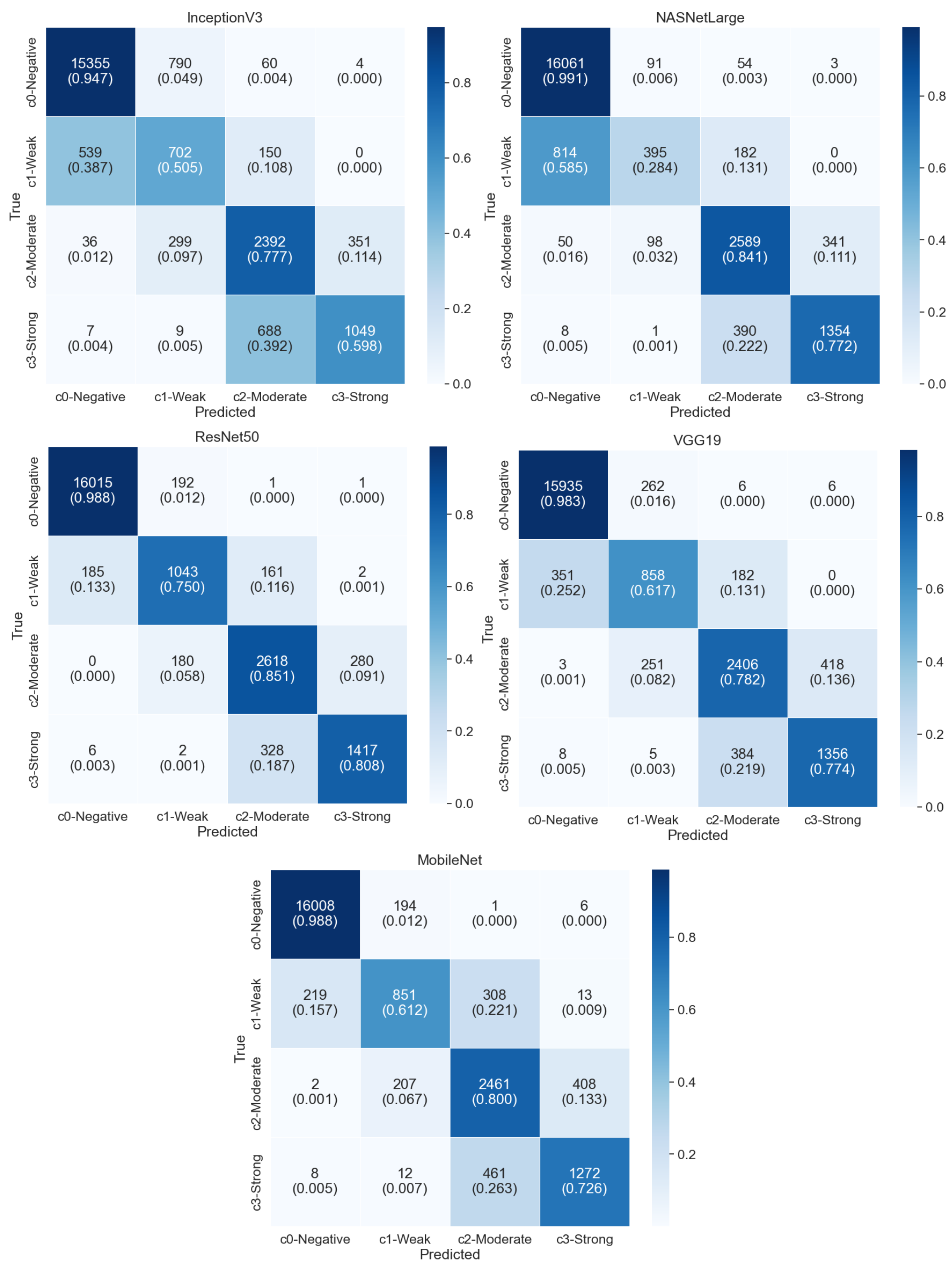
This study employed 32 deep learning architectures from the Keras Applications library [24], initialized with pre-trained weights from ImageNet. Each network incorporates a distinct design for its final classification layer. For instance, DenseNet utilizes an average pooling layer, whereas Xception, ResNet, and Inception models adopt customized dense layers. VGG architectures rely on fully connected layers, while EfficientNet variants incorporate a top dropout layer. MobileNet applies a reshape operation, whereas MobileNetV2 and NASNetMobile employ a global average pooling 2D layer. All models conclude with a Softmax activation function in the output layer to enable multi-class classification. The models are trained with a batch size of 10 and 50 epochs. For the categorization of the four classes, Adam optimizer is used with default parameters, and the categorical cross-entropy loss function is computed. The training images were neither enhanced nor normalized, and accuracy, loss, and computational complexity were used to gauge how well the models trained.

2.3. Ensemble Learning

Deep ensemble learning is generally characterized as the construction of a group of predictions drawn from several deep convolutional neural network models. Ensemble learning depends on integrating data, often through combining predictions, for a single inference. These forecast data may come from a single model, several independent models, or none.

We utilized the 10-fold cross-validation method, generating average probabilities for every 10-fold of the 4 evaluated classes from the individual deep learning models. The three best models were selected from the 32 models for this ensemble stacking based on their highest accuracy.

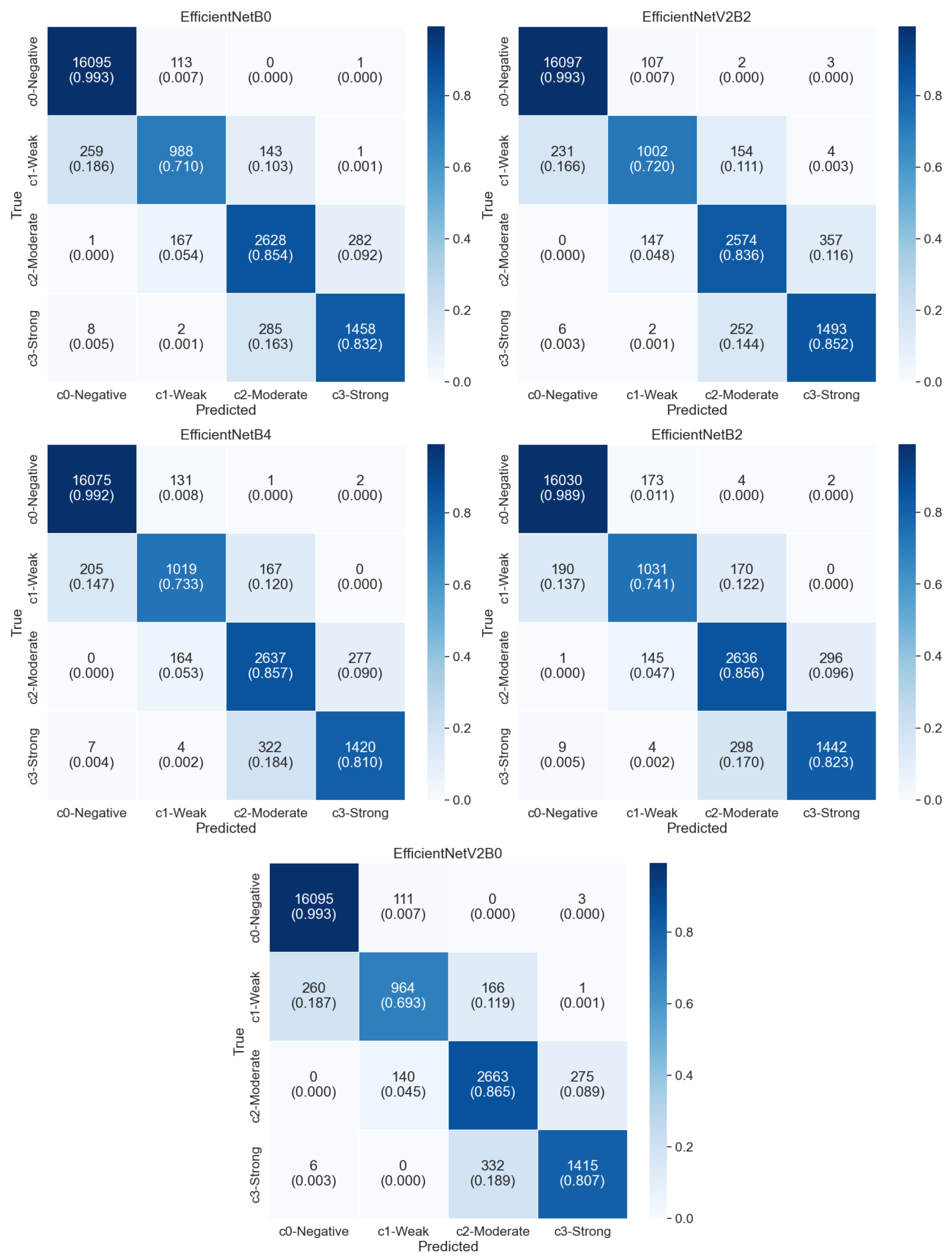
To ensure methodological rigor and avoid information leakage, stacking was performed using out-of-fold predictions. For each fold, the base models (EfficientNetB0, EfficientNetV2B2, and EfficientNetB4) were trained on 9 folds and evaluated on the remaining fold. The predictions from these held-out folds were aggregated across all 10 folds and used to train the logistic regression meta-learner. This ensured that the meta-learner was trained only on predictions from data unseen by the base models.

For the ensemble, logistic regression was chosen as the meta-model for combining predictions. Logistic regression is particularly well suited for this task due to its simplicity and robustness in binary and multi-class classification problems. It provides a probabilistic framework, enabling the integration of predicted probabilities from the base models into a single cohesive prediction. Additionally, logistic regression performs well with limited training data, which is critical for avoiding overfitting when combining predictions from pre-trained models in ensemble learning. This method ensures that the ensemble model remains interpretable and computationally efficient, while leveraging the strengths of the individual base models.

2.4. 10-Fold Cross-Validation

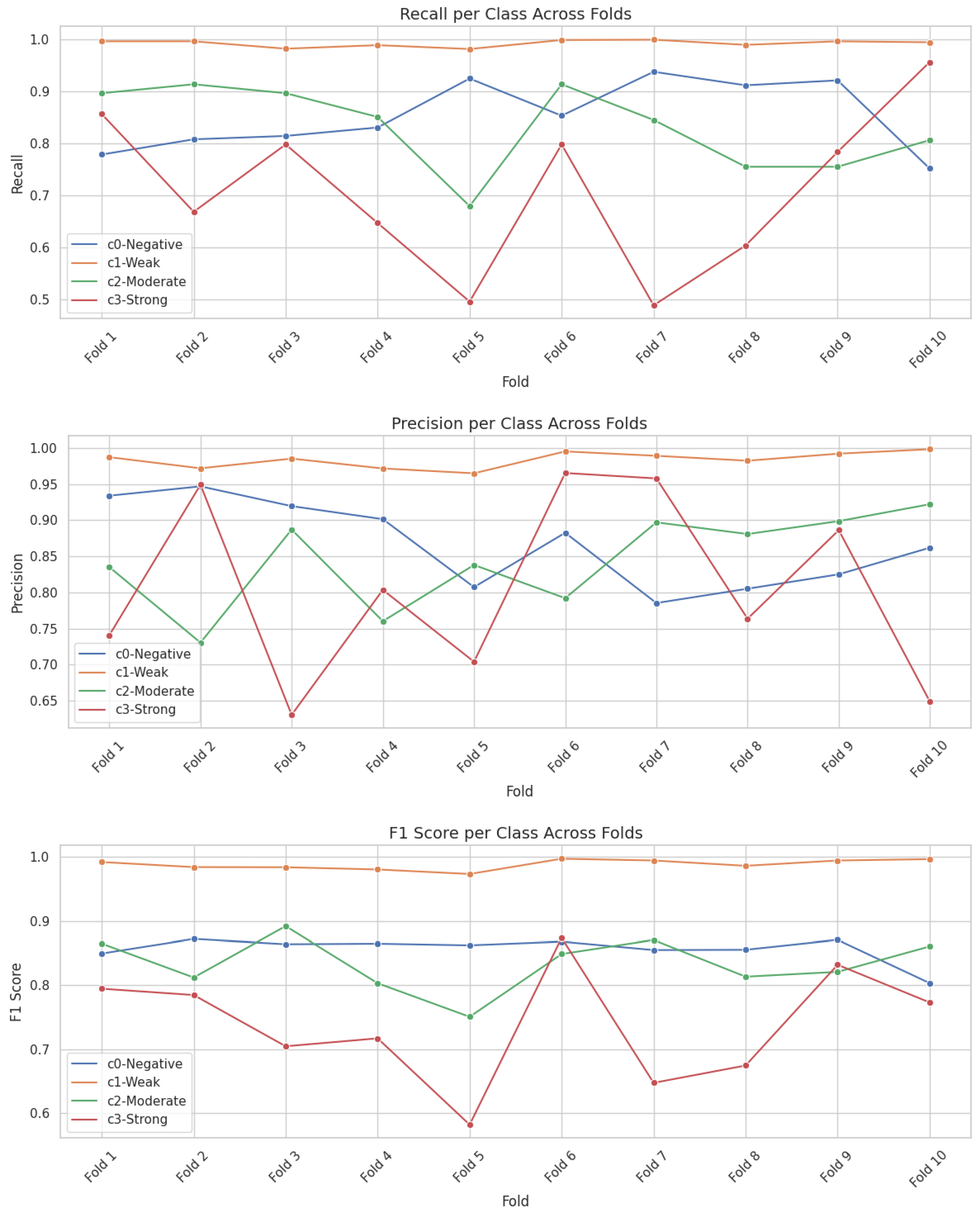
Rather than dividing the dataset of 22,431 nuclei into separate training, validation, and testing subsets, a 10-fold cross-validation strategy was adopted to evaluate both the individual and ensemble models. This approach reduces bias caused by random partitioning, maximizes the utilization of available data, and provides a more reliable estimate of model performance. In this method, the dataset is divided into K = 10 folds; in each iteration, one fold (10%) is used for testing while the remaining folds (90%) are used for training. The process is repeated until every fold has served as the test set once, and the final performance is reported as the average across all folds. Although this strategy enhances the robustness of performance estimation, it cannot replace independent external validation and may still result in overly optimistic generalization outcomes. Additionally, since the folds were generated at the nucleus level, nuclei from the same region of interest (ROI) or slide could appear in both training and testing sets, thereby increasing the risk of data leakage and artificially inflated performance metrics.

2.5. Dataset Evaluation

This study builds upon the findings of our previous work [2], where the classification performance using pre-trained models reached an F1-score of 87.03% and a test accuracy of 94.91%. The earlier dataset was validated by a single pathologist, with two pathologists involved overall, each validating 110 regions of interest (ROIs). To address potential limitations of this validation process and improve the dataset’s quality, we incorporated a methodology that identifies and facilitates the re-evaluation of nuclei misclassified by more than 16 out of 32 models.

2.5.1. Combining Model Results

The first step involved consolidating the outputs from the 32 models. Each model’s results were derived from 10-fold cross-validation, and these individual folds were merged to create a unified dataset per model. The merged datasets were indexed sequentially (1 to 22,000) to maintain consistency and facilitate downstream analysis. This process yielded 32 CSV files, each representing a complete dataset for a model. The consolidated files were integral to subsequent analyses, ensuring that all data points were consistently represented across models.

2.5.2. Creating Comprehensive Datasets (CSV1 and CSV2)

To streamline analysis, two new datasets, CSV1 and CSV2, were constructed:

• CSV1: This dataset recorded whether each model’s prediction was correct or wrong. For each data point, a misclassified_occurrence field was calculated to count the number of models that misclassified it. Data points misclassified by all 32 models were assigned a value of 32.
• CSV2: This dataset captured prediction scores for all models, rounded to four decimal places for precision and readability. These scores were essential for identifying patterns and evaluating model confidence in predictions.

By identifying data points with misclassified_occurrence values greater than 16 in CSV1, we isolated nuclei that warranted re-evaluation. These points, likely representing ambiguous or challenging cases, were targeted for further analysis and expert review.

2.5.3. Identifying and Managing Misclassified Nuclei

Data points with high misclassification frequencies (more than 16 models misclassifying) were flagged, and their corresponding image files were saved into a designated folder named Revalidation. The filenames followed a standardized format, e.g., Index_Originalfilename_misclassifiedOccurrence.png, to ensure traceability and simplify identification during expert review. This approach allowed for a focused re-evaluation of the most problematic cases in the dataset.

2.5.4. Development of a Web-Based GUI for Revalidation

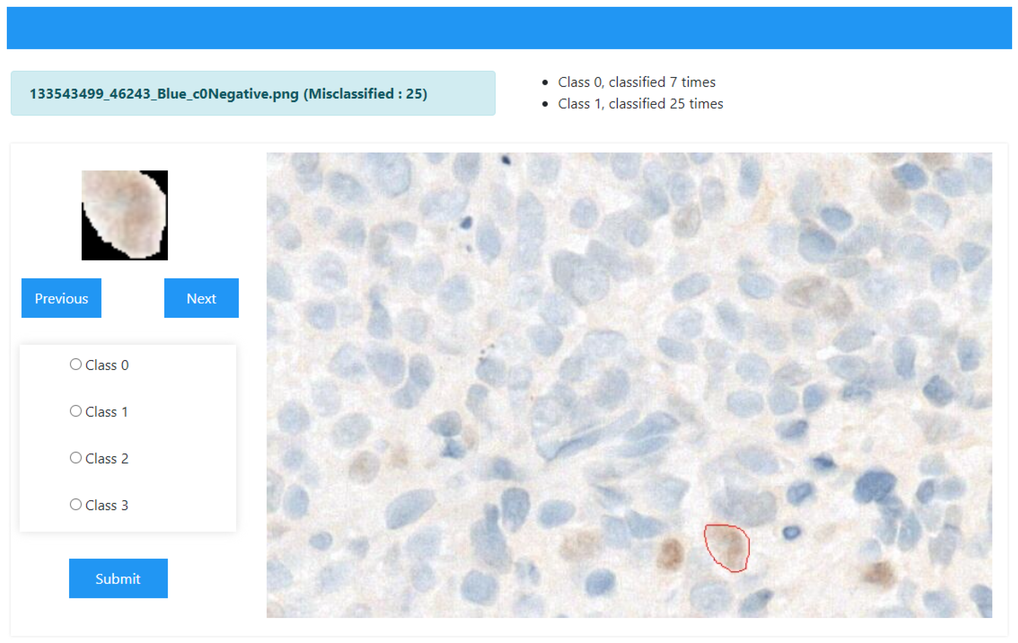
To facilitate the re-evaluation process and actively involve domain experts, a web-based graphical user interface (GUI) was developed using Python 3.9, as depicted in Figure 2. The GUI served as an interactive platform where the results of the 32 pre-trained models could be visualized and assessed. The interface specifically highlighted images misclassified by more than 16 models, enabling pathologists to focus on these challenging cases. This design empowered pathologists to evaluate whether the highlighted misclassifications were accurate reflections of model limitations or indicative of dataset errors.

Key Features of the GUI

The GUI provided several functionalities to enhance usability:

• Image Display: Users could browse and upload nucleus images, which were displayed with their filenames as axis titles. Original ROIs were overlaid using pre-defined coordinates, providing spatial context for each nucleus.
• Prediction Scores: The GUI presented prediction scores from all 32 models in a tabular format. Each model’s scores were displayed with four decimal places, and the highest score in each row was highlighted for clarity.
• Misclassification Summary: A Mostly Predicted As field summarized the class most frequently predicted for the selected nucleus, providing an overview of model consensus.
• Revalidation Panel: The interface included a revalidation panel with radio buttons representing the possible classes (class0 to class3). Pathologists could select the correct class and submit their revalidated classification, which automatically updated the filename (e.g., Index_Originalfilename_misclassifiedOccurrence_reval-newclass.png).

2.5.5. Enhancing Dataset Quality Through Expert Feedback

This interactive platform was instrumental in empowering pathologists to contribute their expertise to the dataset improvement process. By enabling direct correction of misclassified cases, the GUI facilitated the creation of a more accurate and reliable dataset. Pathologists’ active participation ensured that ambiguous or incorrectly labeled data points were addressed, ultimately leading to improved model performance and dataset fidelity.

This methodology underscores the importance of integrating domain expertise into the machine learning workflow. The combination of data-driven analysis and expert feedback fosters iterative improvements, advancing the state of classification analysis and dataset refinement.

3. Experiments and Results

In this section, the results of experiments conducted using 32 pre-trained deep neural networks in transfer learning for breast cancer classification will be presented. The focus of these experiments is on analyzing the performance of these models when applied to histopathological ER-IHC images. Subsequently, the three best-performing models will be utilized in a stacking ensemble learning approach to improve the classification results. The upcoming sections will provide a detailed account of the classification results obtained from these experiments and will also compare these findings with the results reported in other relevant studies. By examining and comparing these results, a comprehensive understanding of the effectiveness of the selected models for breast cancer classification in histopathological images can be gained.

3.1. Model Evaluation

This section presents an extensive analysis of 32 distinct models utilized for classifying our dataset into four categories. The evaluation delves into crucial performance metrics—loss, accuracy, and training time—spanning various architectures. It aims to elucidate the trade-offs observed between model complexity and efficiency. Furthermore, the section explores the results of ensemble-based logistic regression models constructed from the three most promising models among the initial 32.

To assess the training behavior and generalization capability of the top-performing models, we analyzed their learning curves over 50 epochs. Figure 3 presents the training and validation accuracy and loss curves for EfficientNetB0, EfficientNetV2B2, and EfficientNetB4. All three models demonstrate smooth convergence and stable training behavior with minimal signs of overfitting, indicating that the models were effectively optimized and did not exhibit significant divergence between training and validation phases.

Additionally, to investigate the variability in classification performance across the 10-fold cross-validation strategy, we computed per-class metrics—precision, recall, and F1-score—for each fold. Figure 4 illustrates these per-class metrics across folds for the EfficientNetB0 model. The results reveal greater variability in the ‘Weak’ and ‘Strong’ classes, which correlates with their smaller representation in the dataset. These findings highlight the effect of class imbalance and reinforce the need for evaluating model stability beyond aggregate metrics.

The comprehensive analysis provides detailed insights into each model’s performance, highlighting their architectural complexity, number of layers and parameters, classification accuracy, loss, and training time, as summarized in

Table 2. Performance metrics of 32 CNN models with architectural complexity.

Model	Layers	Params	Loss	Accuracy	F1 Score	Training Time (s)
EfficientNetB6	400+	43 M	0.14807	0.93978	0.85	25.69
EfficientNetB7	450+	66 M	0.16901	0.93457	0.83	35.02
EfficientNetV2B2	300+	55 M	0.13644	0.94361	0.86	6.16
EfficientNetV2L	480+	118 M	0.15812	0.94001	0.85	52.97
EfficientNetV2B0	200+	7 M	0.14380	0.94231	0.85	4.35
EfficientNetV2M	360+	54 M	0.16129	0.93366	0.83	24.15
EfficientNetV2S	280+	21 M	0.15547	0.93861	0.84	12.73
EfficientNetV2B3	320+	75 M	0.14745	0.94128	0.85	8.61
EfficientNetB5	300+	30 M	0.15280	0.93972	0.85	19.74
MobileNet	88	4.2 M	0.23682	0.91802	0.79	2.26
ResNet50V2	50	25.6 M	0.89037	0.91458	0.79	5.41
ResNet152	152	60.2 M	0.16802	0.94062	0.85	18.47
ResNet50	50	25.6 M	0.17008	0.94035	0.85	7.11
InceptionV3	48	23.8 M	0.48524	0.86926	0.70	5.04
ResNet101V2	101	44.6 M	1.04735	0.92831	0.82	9.82
NASNetLarge	403	88.9 M	0.25992	0.90941	0.74	1.53
MobileNetV2	88	3.4 M	0.18304	0.93003	0.82	2.70
ResNet101	101	44.5 M	0.17431	0.93863	0.85	12.30
NASNetMobile	350	5.3 M	0.19706	0.92773	0.81	4.12
Xception	126	22.9 M	0.29263	0.92746	0.81	6.05
ResNet152V2	152	60 M	3.20818	0.92434	0.82	19.05
DenseNet201	201	20 M	0.18229	0.93673	0.84	19.86
EfficientNetB0	237	5.3 M	0.14206	0.94372	0.86	5.70
DenseNet169	169	14.3 M	0.17172	0.93945	0.85	14.36
EfficientNetB2	279	7.7 M	0.14033	0.94242	0.85	7.22
DenseNet121	121	8.0 M	0.17744	0.93581	0.84	8.93
EfficientNetB1	250	7.8 M	0.14154	0.94197	0.85	7.71
VGG19	19	143.7 M	0.28179	0.91634	0.79	11.53
EfficientNetB3	300+	12 M	0.16662	0.93785	0.83	10.14
EfficientNetV2B1	250+	8.3 M	0.14887	0.94199	0.85	5.58
VGG16	16	138.3 M	0.27271	0.92234	0.80	9.48
EfficientNetB4	315	19 M	0.14060	0.94294	0.85	14.05

. Figure 5 further visualizes the distribution of accuracy across all models using a box plot representation based on the 10-fold cross-validation strategy.

The evaluation of the 32 models was conducted on a computational setup optimized for deep learning tasks. The specifications of the system used for training and testing the models are as follows:

• Processor: AMD Ryzen 9 5900X 12-Core Processor @ 3.7 GHz
• Graphics Processing Unit (GPU): NVIDIA GeForce RTX 3090 with 24 GB GDDR6X VRAM
• RAM: 16 GB DDR4 @ 3200 MHz
• Storage: 2 TB NVMe SSD for high-speed data access
• Operating System: Ubuntu 20.04 LTS
• Frameworks: TensorFlow 2.10, Keras 2.10.0, and CUDA 11.6

This high-performance system ensured efficient model training and evaluation, enabling precise measurement of training time for each model. The training time values presented in Table 2 were recorded using this setup under consistent environmental conditions to ensure reliability and reproducibility.

The table provides a comprehensive overview of various models sorted by their F1-score. Among the models listed, the EfficientNetB0 model stands out as it achieves a relatively high accuracy of 94.37% with a low loss of 0.142 while maintaining a remarkably low training time of 5.7 s. Similarly, EfficientNetV2B2 performs exceptionally well with a loss of 0.136, an accuracy of 94.36%, and a short training time of 6.16 s. The highest five models’ confusion matrices are shown in Figure 6. These models showcase a balance between performance metrics and efficiency in training. As the complexity increases with models like EfficientNetV2L and EfficientNetB7, there is a slight trade-off seen in their training times, which exceed 50 s while maintaining decent accuracy rates around 94% and 93.45%. In contrast, models such as MobileNet, while having significantly lower parameters, show higher losses (0.23682) and relatively lower accuracy (91.80%) compared to EfficientNet variants.

The ResNet and DenseNet architectures occupy intermediate positions in terms of both complexity and performance, demonstrating decent accuracy scores ranging from approximately 91% to 94% with varying training times. On the other hand, InceptionV3 achieved the lowest accuracy score of 86.92%. The five lowest models’ confusion matrices are shown in Figure 7. The results indicate that the EfficientNet series, specifically EfficientNetB0, EfficientNetV2B2, and EfficientNetB4, demonstrate superior performance in terms of accuracy, achieving scores above 94%. These models also exhibit relatively lower loss values compared to others, indicating a better fit to the training data. Interestingly, the EfficientNet models with higher parameter counts, such as EfficientNetV2L and EfficientNetB7, do not necessarily yield better results. This suggests that while a higher number of parameters may allow for more complex representations, it does not always guarantee improved performance. It highlights the importance of efficient model architecture design, as observed in EfficientNetB0, which achieves excellent performance despite having fewer parameters. Comparing the different architectures, it can be noted that EfficientNet models generally perform better than ResNet, DenseNet, VGG, MobileNet, and NASNet models in terms of accuracy. This indicates the effectiveness of the EfficientNet architecture in achieving higher accuracy while maintaining a reasonable number of parameters and model sizes.

In our prior publication, as documented in [2], DenseNet169 exhibited an accuracy of approximately 94.91%. However, in this present paper, the reported accuracy stands at 93.94%. The disparity in performance can be attributed to a methodological distinction: the previous study employed a testing dataset comprising only 20% of the available data, while the current research utilizes a more robust approach involving a 10-fold cross-validation method. This alteration in methodology likely contributed to the observed reduction in accuracy.

In ensemble learning, we use the stacking method. We use the 3 best models based on accuracy EfficientNetB0 94.37%, EfficientNetV2B2 94.36%, and EfficientNetB4 94.29%. Using these 3 model values find the stacking value and then apply that value to the logistic regression method to train again. After that, we test with a k-fold test set. The total accuracy of logistic regression was 95% which is better than any of the 32 models. Figure 8 shows the confusion matrix of logistic regression.

3.2. Nuclei Analysis for Dataset Evaluation

We assess our dataset by subjecting each nuclei test as individual test data through a 10-fold cross-validation technique employing our set of 32 trained models as well as the ensemble model. Whenever more than 16 models misclassify the nuclei, we make a remark to the nuclei as “incorrectly labeled nuclei” and require revalidation by the pathologist. From the analysis, we have identified a total of 1406 nuclei that need revalidation. These “incorrectly labeled nuclei”, along with their corresponding Regions of Interest (ROIs), are presented in the developed web-based GUI. The GUI platform not only displays the misclassified nuclei but also highlights their positions within the ROIs. This platform enables pathologists to review the identified nuclei, assign a new class directly through the GUI, and update the ground truth database. The GUI further facilitates this process by offering navigation buttons for pathologists to cycle through different nuclei instances, providing an intuitive method for making adjustments using the “next” and “previous” buttons.

4. Conclusions

In conclusion, this study conducted extensive analysis of 32 pre-trained deep learning models from Keras Applications, evaluating their performance in classifying negative, weak, moderate, and strong nuclei in ER-IHC-stained histopathology images. The primary focus of this study is to provide a complete workflow from deep learning model analysis to identify recurring misclassifications that are possibly “incorrectly labeled nuclei” of the ground truth database. This will facilitate easy rectification and revalidation of the identified images by the pathologist using a user-friendly web-based platform without having to go through the large dataset again. In addition to that, a stacking ensemble model was established using a stacking approach, combining the top three models.

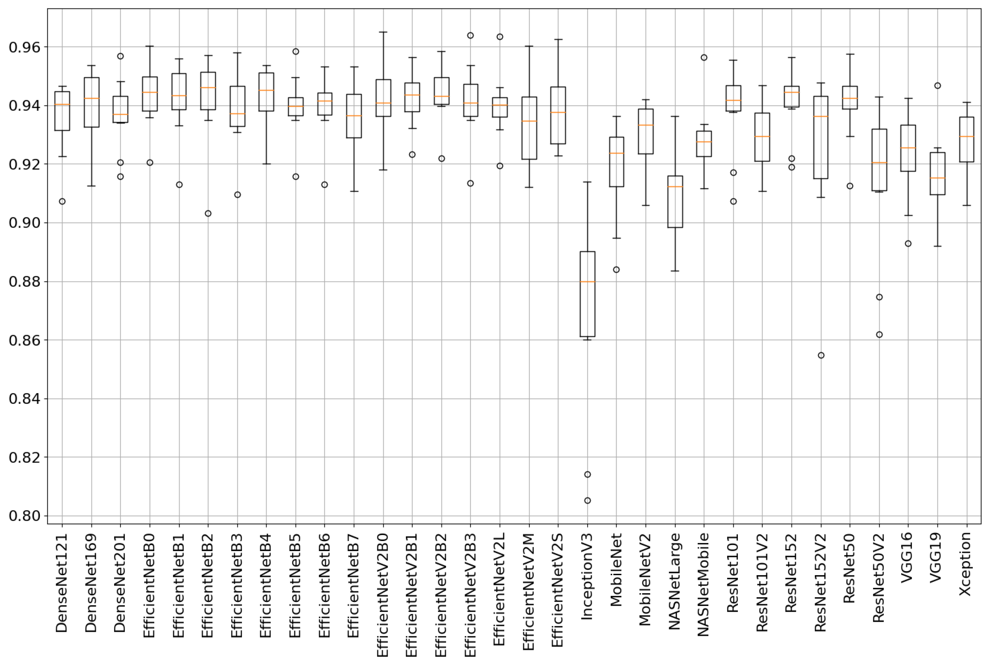
The analysis revealed that the top three performing models were EfficientNetB0, EfficientNetV2B2, and EfficientNetB4, achieving accuracies of 94.37%, 94.36%, and 94.29%, respectively. An ensemble model created using logistic regression with these three models resulted in an improved accuracy of 95%.

This work demonstrates significant potential for enhancing medical image analysis, particularly in addressing intra-observer variability in ground truth validation for large datasets. The findings provide a solid foundation for developing optimized models for nuclei classification in histopathology images and can facilitate more accurate recommendations for hormonal therapy. Moving forward, it would be valuable to explore patient-based classification and investigate other promising models, aiming for even higher accuracy and performance on more challenging datasets. The potential future development of intricate or simplified cascading models could further improve the classification of ER-IHC-stained images.

Despite the promising results, this study has several limitations. First, all performance estimates were obtained using 10-fold cross-validation without an independent hold-out test set, which may lead to optimistic metrics. Second, because cross-validation was conducted at the nucleus level, nuclei from the same ROI or slide could appear in both training and testing folds, potentially causing data leakage and inflating performance. Third, the dataset was derived from a single institution, and no external validation was performed. As a result, generalizability to other cohorts may be affected by domain shift due to variations in staining protocols, scanners, and population characteristics. Future work should address these limitations by employing patient- or slide-level splits and validating on independent multi-center datasets.