Article

A Lightweight Deep Learning Model for Automatic Modulation Classification Using Dual-Path Deep Residual Shrinkage Network

College of Computer Science, Engineering and Technology, Colorado Technical University, Colorado Springs, CO 80907, USA
*
Author to whom correspondence should be addressed.
AI 2025, 6(8), 195; https://doi.org/10.3390/ai6080195
Submission received: 14 July 2025 / Revised: 6 August 2025 / Accepted: 12 August 2025 / Published: 21 August 2025
(This article belongs to the Section AI Systems: Theory and Applications)

Abstract

Efficient spectrum utilization is critical for meeting the growing data demands of modern wireless communication networks. Automatic Modulation Classification (AMC) plays a key role in enhancing spectrum efficiency by accurately identifying modulation schemes in received signals—an essential capability for dynamic spectrum allocation and interference mitigation, particularly in cognitive radio (CR) systems. With the increasing deployment of smart edge devices, such as IoT nodes with limited computational and memory resources, there is a pressing need for lightweight AMC models that balance low complexity with high classification accuracy. In this study, we propose a low-complexity, lightweight deep learning (DL) AMC model optimized for resource-constrained edge devices. We introduce a dual-path deep residual shrinkage network (DP-DRSN) with garrote thresholding for effective signal denoising, and we designed a compact hybrid CNN-LSTM architecture comprising only 27,072 training parameters. The proposed model achieved average classification accuracies of 61.20%, 63.78%, and 62.13% on the RML2016.10a, RML2016.10b, and RML2018.01a datasets, respectively, demonstrating a strong balance between model efficiency and classification performance. These results highlight the model’s potential for enabling accurate and efficient AMC on edge devices with limited resources, despite not surpassing state-of-the-art accuracy owing to its deliberate emphasis on computational efficiency.

1. Introduction

Spectrum is a limited and valuable physical resource, and its efficient utilization is essential to support the growing data demands of wireless communication networks. In the dynamic landscape of modern communication systems, maximizing radio spectrum efficiency is paramount. Automatic Modulation Classification (AMC) is a key technology that significantly contributes to this goal. By enabling receivers to accurately identify the modulation scheme of incoming signals, AMC supports dynamic spectrum allocation and optimizes the use of available radio frequencies. This capability is particularly critical in cognitive radio (CR) systems, where secondary users must access the spectrum without interfering with primary users [1]. Accurate modulation recognition enables systems to adjust transmission parameters according to current channel conditions, thereby optimizing data throughput within the allocated bandwidth.
The study of AMC is vital for industries such as telecommunications, satellite communication, IoT, smart device development, and military applications. AMC aids in signal intelligence, electronic warfare, and secure communication [2]. The telecommunications industry benefits from AMC’s role in enhancing spectrum efficiency, mitigating interference, and managing dynamic spectrum to support data growth in congested wireless environments [3]. Internet of Things (IoT) and smart device developers can use lightweight AMC models for efficient data transmission and energy-efficient communication.
Technologies, such as IoT, medical sensors, and smart home systems, have advanced rapidly. A growing number of small devices require wireless communication in complex, noisy environments. To meet the demand for real-time performance and low complexity, DL models must be developed for faster and more efficient AMC solutions targeting edge devices like IoT [4].
Previous studies have predominantly focused on utilizing more complex neural network structures to extract diverse signal features, thereby enhancing recognition accuracy. However, this has resulted in larger model sizes and increased computational demands, requiring hundreds of thousands to millions of parameters, which are unsuitable for resource-constrained edge receivers. Simultaneously, efforts to simplify DL-based models often compromise recognition accuracy, making it challenging to meet the requirements of edge devices in modern communication systems.
This study proposes a low-complexity, lightweight DL AMC model for edge network devices with limited memory and computing resources. The key contributions of this work are as follows:
  • We introduce the application of a dual-path deep residual shrinkage network (DP-DRSN) for AMC.
  • We create an efficient hybrid convolution neural network (CNN) and Long Short-Term Memory (LSTM) model using only 27k training parameters.
  • We enhance AMC recognition accuracy by integrating a self-learnable scaling approach for signal denoising thresholds, leveraging garrote thresholding to balance denoising effectiveness, model performance, and computational complexity.
We trained and experimented with standard datasets, RML2016.10a, RML2016.10b [5], and RML2018.01a [6], which have been widely used in prior AMC research. The proposed model utilizes only 27k parameters and performs 2.36 million to 18.82 million floating-point operations per second (FLOPs), and is 108.83 kB in size, achieving an inference time of 1.04 ms per sample and an energy usage of 31.5 mJ per sample. Using the RML2016.10a, RML2016.10b, and RML2018.10a datasets, it achieves an average classification accuracy of 61.20%, 63.78%, and 62.13%, respectively.
This manuscript is organized as follows: Section 2 reviews related work; Section 3 presents the problem statement, hypothesis, and research question; Section 4 outlines the methodology and the proposed AMC model design; Section 5 details the datasets, experiments, analysis of results, and ablation studies; Section 6 provides discussion, limitations, and recommendations for future research; and Section 7 concludes the study.

2. Related Work

The need for lightweight AMC models to support edge devices, such as IoT and CR systems, is becoming increasingly critical. However, balancing computational efficiency and classification accuracy remains a significant challenge in resource-constrained, interference-prone, and spectrum-dense environments. Several recent studies have proposed innovative approaches to address these challenges.

2.1. Models with <5ok Tunable Parameters

Lin et al. [4] introduced a novel lightweight AMC model using Liquid State Machine (LSM) spiking neural networks (SNNs) with 7120 parameters, achieving faster processing but lower average accuracy (36.69–79.68%) for RML2016.10a, RML2016.10b, and RML2018.01a datasets. Ke and Vikalo [7] proposed a compact LSTM-based denoising auto-encoder with 14,637 parameters to classify modulation and technology types from noisy radio signals, achieving a Top-1 accuracy of 61.72% on the RML2018.01a dataset. However, since Top-1 accuracy overlooks class imbalance, the more equitable average classification accuracy was recalculated as 58.74% to enable fairer model comparisons. In [8], Shaik and Kirthiga used DenseNet with 19k parameters, showing 55–70% accuracy for RML2018.01a. TianShu et al.’s [9] Long-term Features Neural Network (IQCLNet) classifier with I/Q correlator had 29k parameters, reaching 59.73% accuracy for RML2016.10a. Shen et al. [10] developed a multi-subsampling self-attention network (MSSA) using dilated convolution branches with self-attention, with variants from 36k to 218k parameters, achieving 55.25–60.90% accuracy for Unmanned Aerial Vehicle (UAV)-to-ground communication systems. An et al. [11] proposed the Threshold Denoise Recurrent Neural Network (TDRNN) model, consisting of two key components: a Threshold Denoiser (TD) module using soft thresholding to filter out noise from received signals, and a GRU layer to classify the denoised signals. The TDRNN model has 41k parameters and an average accuracy of 63.5%, using the RML2016.10a dataset.
Gao et al. [12] built upon their previous work in [13] and developed a lightweight modulation recognition algorithm based on a CNN-LSTM dual-channel model, addressing class imbalance through data preprocessing. The algorithm reduced the number of parameters from 44,379 to 43,941, achieving 66.7% accuracy for five selected modulations on the balanced RML2016.10a dataset and 64.2% in imbalanced scenarios (20:1 ratio). Li et al. [14] proposed a complex-valued transformer (CV-TRN) model using complex multi-head self-attention. With 44,790 parameters, CV-TRN achieved 63.74% accuracy on RML2016.10a and 64.13% on RML2018.01a. However, its reliance on relative position embedding and phase offset data augmentation adds complexity to its deployment. Su et al. [15] proposed SigFormer, a robust signal classification model using a pyramid Transformer architecture, achieving 63.71% (RML2016.10a), 65.77% (RML2016.10b), and 63.96% (RML2018.01a) with models of 44k, 44k, and 158k parameters, respectively.

2.2. Models with 50k to 100k Tunable Parameters

Ding et al. [16] addressed the limitations of pure data-driven AMC methods by incorporating expert knowledge to improve recognition in high-noise conditions. They used CNN, specifically ResNet, with a Bidirectional GRU (BiGRU), with dual-driven schemes combining data-driven and semantic knowledge approaches. With 69k parameters, the model achieved 100% accuracy at >2 dB SNR and 34% at −10 dB for the RML2018.01a dataset. Zhang et al. [17] developed a model using CNN and GRU layers for feature extraction and achieved 60.44–63.82% accuracy across different datasets. They proposed model pruning using TensorFlow’s Keras tool, maintaining high accuracy for RML2016.10a/b but showing a drop for RML2018.01a. Guo et al. [18] proposed an SNN-based classification method using ΣΔ spike encoding, achieving up to 64.29% accuracy with 84k–627k parameters. Li et al. [19] proposed a lightweight multi-feature fusion structure (lightMFFS) CNN architecture for AMC, with an asymmetric convolution structure and attention-based fusion mechanism, achieving 63.44–65.44% accuracy for RML2016.10a/b with 95k parameters and 0.34 million FLOPs.

2.3. Models with 100k to 250k Tunable Parameters

Zheng et al. [20] introduced a Transformer-based automatic modulation recognition (TMRN-GLU) model leveraging CNN and RNN for modulation classification. TMRN-GLU achieved 65.7% average accuracy and 93.7% max accuracy on RML2016.10b with 106k parameters. A smaller version, TMRN-GLU-Small, had 25k parameters with 61.7% accuracy. Ning et al. [21] proposed a transformer-based model, MAMR, leveraging multimodal fusion of I/Q and Fractional Fourier Transform (FRFT) signals to improve classification robustness, achieving an average accuracy of 61.55% and 79.01% on the RML2016.10a and HisarMod2019.1 datasets with 100k model parameters. Its reliance on computationally expensive FRFT transformations remains challenging. Shi et al. [22] proposed a depthwise separable CNN with self-attention, achieving 98.7% maximum classification accuracy on RML2018.10a with 113k parameters. Xue et al. [23] proposed MLResNet, an improved ResNet with an LSTM DL network architecture of parameter size of 115k, achieving a maximum accuracy of 96% at 18 dB for the RML2018.01a dataset. Riddhi et al. [24] created a hybrid CNN-GRU model with an attention mechanism. Despite using fewer layers and filters, the architecture still comprises 145k tunable parameters, achieving an accuracy of over 96% at high SNRs and over 75% at lower SNRs (−4 dB to 18 dB) for digital modulation types.
Parmar et al. [25] proposed a dual-stream CNN-BiLSTM model, achieving an average 68.28% accuracy on RML2016.10b for digital modulation types using 145k tunable parameters, demonstrating an effective balance between feature extraction and model size. In [26], Parmar et al. introduced a multilevel classification approach with three DL models (AD-MC, An-MC, and Dig-MC) to classify signals into analog or digital categories and classify specific modulation types. While this approach demonstrated superior performance at higher SNRs, it required 155k parameters and achieved an average accuracy of 63% on the RML2016.10b dataset, balancing complexity with moderate performance improvements. Chang et al. [27] introduced the Fast Multi-Loss Learning Deep Neural Network (FastMLDNN), which stacks three group convolutional layers and a transformer encoder to improve feature extraction while minimizing the risk of overfitting. The proposed model reduces computational overhead nearly nine times compared to its baseline, MLDNN [28], achieving 63.24% average accuracy for RML2016.10a with 159k parameters. Luo et al. [29] developed RLITNN for low-SNR recognition, integrating LSTM and Transformer-encoder modules, multi-head attention mechanisms, and multiple feature extraction modules for amplitude, phase, spectrum, and power spectral density. The model required 181k parameters and 53.75 million FLOPs, achieving 63.84% (RML2016.10a) and 65.32% (RML2016.10b) average accuracy. Harper et al. [30] focused on differentiable statistical moment aggregation for feature learning, using fixed and learnable moments to refine modulation scheme representations using CNN architecture with squeeze and excitation (SE) blocks. With 200k parameters, it has an average of 63.15% and a maximum of 98.9% accuracy using RML2018.01a with a high computational overhead. In [31], Harper et al. integrated CNN architecture with dilated convolutions, statistics pooling, and SE units. It achieved peak accuracy with 202k tunable parameters of 98.9% and an average accuracy of 63.7% on the RML2018.01a dataset. Huynh-The et al. [32] proposed a cost-effective and high-performance CNN model, MCNet, comprising 220k parameters and achieving a classification accuracy of over 93% at 20 dB SNR for the RML2018.10a dataset. In [33], Sun and Wang developed a Fusion GRU DL Neural Network (FGDNN) combining GRUs and CNNs to enhance spatiotemporal feature extraction, and the model achieved 90% accuracy at 8 dB SNR with 253k parameters. Nisar et al. [34] utilized ResNet blocks and SE networks to improve AMC’s accuracy and efficiency. Their model, with 263,000 parameters and 749 million FLOPs, achieved accuracies of 81% (18 dB) using the RML2016.10a dataset.
Table 1 shows the model performance in ascending order by tunable parameter size, including the proposed model presented in this study for comparison. It can be observed that classification accuracy improves as model complexity increases and vice versa.

3. Problem Statement, Hypothesis, and Research Question

3.1. Problem Statement

The problem is that achieving high classification accuracy in DL models for AMC necessitates increased model complexity. This complexity renders these models unsuitable for deployment on widely distributed edge devices, such as IoT, medical sensors, and smart home systems, which are constrained by limited memory and computational resources. Efforts to reduce DL model complexity often result in compromised classification accuracy, creating a critical challenge for the effective deployment of AMC in edge environments.

3.2. Hypothesis

If we can develop a novel DL model for AMC tailored for edge devices, which harmoniously balances high modulation classification accuracy and low model complexity in an overcrowded and noisy wireless environment, then we can effectively tackle the challenge of creating efficient DL AMC models for edge devices.

3.3. Research Question

How can advanced lightweight AMC models be designed to optimize classification accuracy and model complexity for resource-constrained edge devices?

4. Methodology and Proposed Model

4.1. Methodology

Modulating a baseband signal encoded with input data into a high-frequency carrier signal transmitted over the air channel is called modulation. In a typical modern wireless communication system, the transmitted signal is dynamically modulated based on channel conditions and the specifications of the system [35]. The primary method of conducting modulation classification consists of deploying a DL classification model on incoming propagation signals at the radio receiver of the wireless network. The objective of AMC can be described mathematically by (1), where y ^ represents the predicted modulation type, y represents the actual modulation type, and W represents the learned weights of the DL model.
y ^ = a r g m a x f y X ; W
Incoming propagation signals are represented by X is an input feature that represents in-phase and quadrature-phase (I/Q) baseband signals. In a single-input single-output (SISO) system, the received signal can be expressed as shown in (2). s t represents the modulated signal, h t denotes the channel impulse response, and n t accounts for noise.
x t = s t h t + n t
The modulation signals take on different forms depending on the type of modulation. To simplify subsequent signal processing and modulation recognition, the received signal is typically represented by in-phase and quadrature (I/Q) components [36].
As a result, the I/Q signal can be described as a 2 × N matrix, as shown in (3):
X I Q = X I x 1 , X I x 2 X I x N X Q x 1 , X Q x 2 X Q x N
The first row of X I Q corresponds to the in-phase component (I vector), while the second row represents the quadrature component (Q vector). XI and XQ represent the in-phase and quadrature-phase components, respectively, and N is the length of the sample.
In [33], Sun and Wang demonstrated that modulated signals not only have temporal but also has spatial characteristics. They show that the amplitude and phase of the modulated signal improve AMC modulation classification. Thus, amplitude/phase (A/P) data was generated by converting in-phase/quadrature (I/Q) data from the Cartesian coordinate system to the polar coordinate system shown in (4) and (5). X A P is used as input in the proposed model shown in (6).
A i = X I 2 i + X Q 2 i
P i = a r c t a n ( X I [ i ] X Q [ i ] )
X A P = A x 1 , A x 2 A x N P x 1 , P x 2 P x N
X A P represents a 2 × N vector of amplitude and phase, where A represents the amplitude vector, and P represents the phase vector.

4.2. Signal Denoising

Wireless signals are inherently susceptible to noise and interference, which can significantly distort the transmitted information and degrade signal quality. This vulnerability necessitates robust signal processing techniques to mitigate noise-induced impairment for reliable demodulation.
In wireless signal denoising, the task is to recover the actual signal coefficient θ from a noisy observation x , where x = θ + ϵ , where ε is assumed to be noise. Two estimators used in this context are soft thresholding and garrote thresholding. Soft thresholding is defined by (7),
θ ^ s x =   0 ,                                                                 x < τ ( x τ ) . S g n x ,               x   τ
which subtracts a fixed threshold τ from the magnitude of x when | x | τ , resulting in a constant bias of approximately τ for large true coefficients. In contrast, the garrote thresholding estimator θ ^ G x , given by (8), can be rewritten as (9).
θ ^ G x = 0 ,                                                                           x < τ x τ 2 x ,                                               x   τ
θ ^ G x = 0 ,                                                                           x < τ   x 1 τ 2 x 2 ,                                       x   τ
Garrote thresholding operates by scaling x with a factor that depends inversely on the square of x , thereby reducing the bias in proportion to the magnitude of the true signal. A more detailed bias analysis demonstrates that for soft thresholding, when x is close to the true coefficient θ ( θ > τ ) . The soft threshold estimator θ ^ s x can be approximated as shown in (10).
θ ^ s x θ s g n θ τ
This implies a bias of roughly τ . On the other hand, the garrote estimator under the assumption x θ is approximated by (11) and rewritten as (12).
θ ^ G x θ ( 1 τ 2 θ 2 )
θ ^ G x = θ τ 2 θ
Its bias is thus τ 2 θ , notably smaller than τ when θ > τ . This reduction in bias directly contributes to a lower mean-squared error (MSE), as MSE comprises the squared bias and the variance of the estimator.
From the perspective of MSE, soft thresholding’s fixed shrinkage introduces a persistent bias that may dominate the error of significant signal components, leading to potential degradation in performance when denoising signals with large coefficients. In contrast, the adaptive bias of garrote thresholding decreases with increasing θ , ensuring that high-magnitude coefficients often present in a wireless communication system that tends to be sparse and bursty are preserved more accurately.
Moreover, as shown in Appendix A.1, the smooth transition of the garrote function around the threshold helps to avoid the abrupt discontinuities inherent in soft thresholding, which can otherwise generate artifacts in the denoised signal. Overall, in wireless signal denoising, where preserving a large magnitude, an informative coefficient is essential, the garrote thresholding method demonstrates a mathematical advantage over soft thresholding with minimal increase in computational cost. Its reduced bias for significant components, consequent improvement in overall MSE, and smoother functional behavior justify its preference for applications that demand high fidelity in signal recovery.
Additionally, the DP-DRSN, as described in Appendix A.1, is employed to enhance denoising effectiveness by leveraging both global average pooling (GAP) and global maximum pooling (GMP) to estimate adaptive thresholds. In contrast to the DP-DRSN, the single-path deep residual shrinkage network (SP-DRSN), as described in Appendix A.3, relies solely on GAP. DP-DRSN captures both the average contextual information and the prominent high-amplitude signal features that often signify transient noise. The denoising threshold is computed using a learnable convex combination as shown in (14), where α and β are derived from GAP and GMP, respectively, γ   ϵ   [ 0,1 ] is a learnable weight, and self-learning κ scales the combined threshold.
T h r e s h o l d = κ ( γ α + 1 γ β )
This formulation allows the model to dynamically adjust denoising sensitivity during training, thereby enhancing robustness in heterogeneous and noisy environments.

4.3. Proposed Model

The proposed model has three blocks: feature extraction, denoiser, and classifier. The choices in the model layer parameters are intended to minimize the model’s weight while maximizing its accuracy. The proposed model architecture description is provided in Appendix A.

5. Experiments and Result Analysis

5.1. Dataset

There are many publicly available datasets that researchers have used in previous AMC studies, such as the narrow-band radio machine learning (RML) datasets proposed by O’Shea et al., namely RML2016.10a, RML2016.10b [5], RML2018.01a [6], and HisarMod2019.1 [37]. This study utilizes RML2016.10a, RML2016.10b, and RML2018.01a to compare the performance of the proposed model with that of previous research. Table 2 provides details of datasets, including training, validation, and testing configurations. The training, validation, and test sets were generated using stratified random sampling to ensure uniform sampling across all SNR levels and across all modulation types. To enhance reproducibility, all experiments were conducted with a fixed random seed. This method ensures that each class and SNR condition is equally represented in each subset of training, validation, and sample data, promoting balanced learning and evaluation.
The RML2016.10a dataset contains a total of 220,000 samples across 20 SNR levels ranging from −20 dB to +18 dB, and it includes 11 modulation schemes: AM-DSB, AM-SSB, WBFM, BPSK, QPSK, 8PSK, 16QAM, 64QAM, GFSK, CPFSK, and PAM4. The RML2016.10b dataset is a larger and more advanced benchmark for AMC, comprising 1.2 million samples across 10 modulation schemes: AM-DSB, WBFM, BPSK, QPSK, 8PSK, 16QAM, 64QAM, CPFSK, GFSK, and PAM4.
Additionally, RML2018.01a is used for further testing and an ablation study to evaluate parameter size, FLOPs, energy usage, and classification benchmarking. The RML2018.01a dataset is the prominent benchmark for modulation recognition. Its broad diversity and representative qualities make it ideal for AMC research. The RML2018.01a dataset brings in newer modulation classes, increased signal complexity, and the evolving need for modulation recognition research [38]. RML2018.01a has 24 modulations (8PSK, BPSK, CPFSK, GFSK, PAM4, AM-DSB, 16QAM, 64QAM, QPSK, WBFM, OOK, 4ASK, BPSK, QPSK, 8PSK, 16QAM, AM-SSB-SC, AM-DSB-SC, FM, and GMSK), a signal dimension of 2 × 1024, and an SNR range of −20 dB to 18 dB at 2 dB increments. There are 2,555,904 samples, with 4096 samples for each modulation and SNR (i.e., 24 modulations × 26 SNR levels × 4096 equates to 2,555,904 samples). To simulate real-world scenarios, the signals are distorted with impairments such as sample rate offset, center frequency offset, symbol rate offset, selective fading, and additive white Gaussian noise (AWGN).

5.2. Experimental Setup

The training process hyperparameters were set to a batch size of 64 and an initial learning rate of 0.001, with beta_1 = 0.9 and beta_2 = 0.999, using the Adam optimization algorithm. The training was run for 200 epochs, with the learning rate halved if the validation loss remains unchanged after five epochs. Using the EarlyStopping procedure, the training process stops if the validation loss does not decrease after 30 epochs. The experiments were conducted on a Windows 11 machine equipped with an Intel Core i9-2600 MHz processor, 64 GB RAM, and an NVIDIA GeForce RTX 4080 GPU. Keras and TensorFlow were used to train the model.

5.3. Testing and Training Results

The total number of model-trainable parameters is only 26,638 for the RML2016.10a and RML2016.10b datasets and 27,072 for the RML2018.01a dataset. This lightweight model achieves high average classification accuracy while minimizing the complexity of the model architecture. As shown in Table 3 and Table 4, the proposed model’s classification accuracy and model complexity are provided, measured according to trainable parameters, FLOPs, inference time per sample (ms), memory usage (GB), and energy usage (mJ) per sample. Memory usage represents the NVIDIA GeForce RTX 4080 GPU run-time memory consumption during model inference, as measured using the TensorFlow memory profiler. Note that by default, TensorFlow allocates all available GPU memory during inference, resulting in consistent memory usage across different models reported in this study. Overall, an average modulation classification accuracy of 61.20%, 63.78%, and 62.13% and a maximum classification accuracy of 91.23%, 93.64%, and 97.94% were achieved for RML2016.10a, RML2016.10b, and RML2018.01a, respectively. A training and validation loss plot is shown in Figure 1, while the classification accuracy at each SNR level is shown in Figure 2.
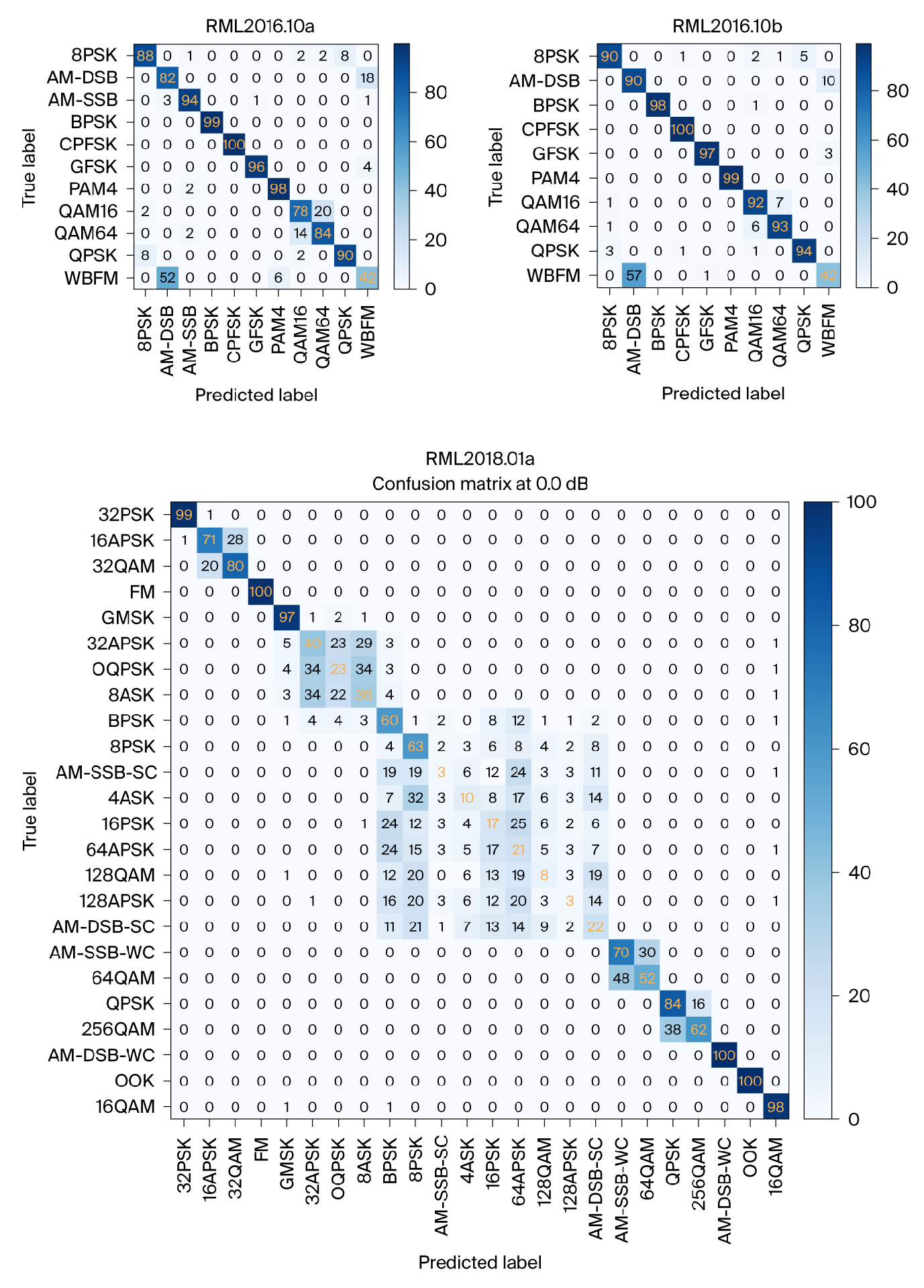
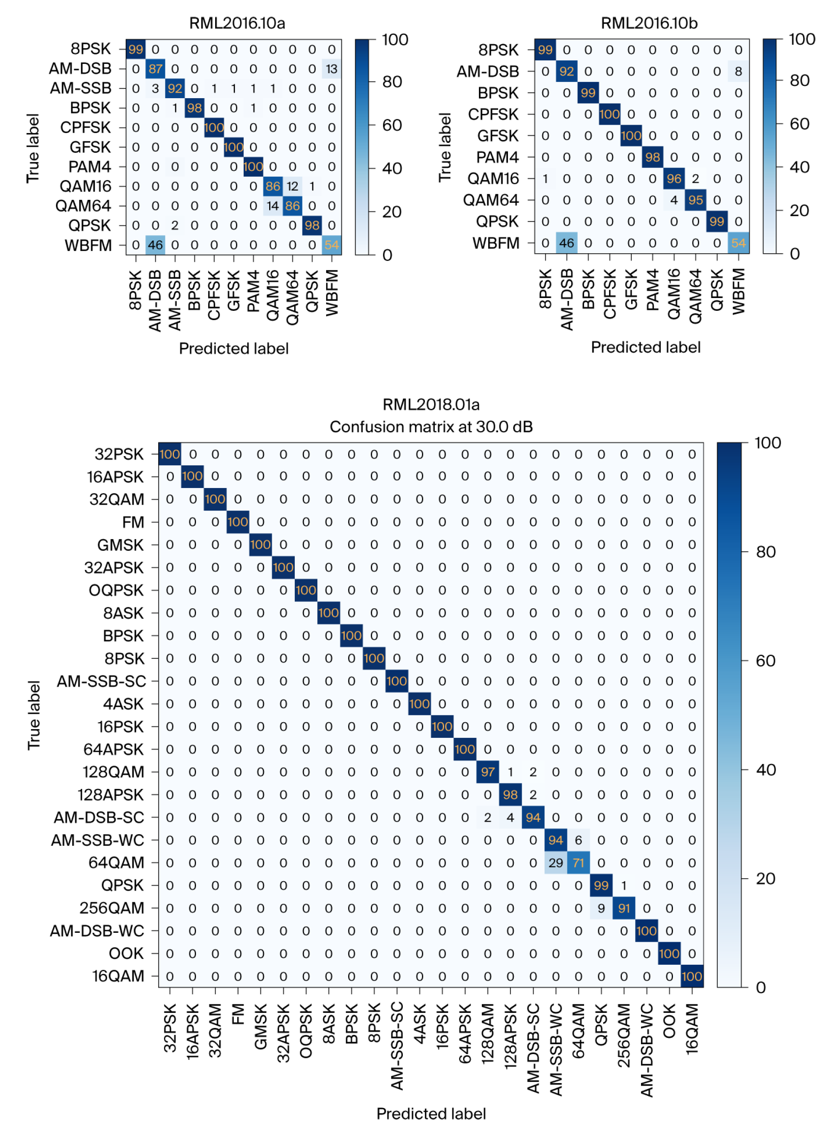
In addition, a confusion matrix analysis was performed at each SNR level. Figure 3 shows the confusion matrix at 0 dB, and Figure 4 shows the confusion matrix at 18 dB for RML2016.10a and RML2016.10b, and at 30 dB for the RML2018.01a dataset. The other aspect of the DL model complexity evaluation entails the model’s inference time, energy usage, and FLOPs. The FLOPs vary based on the size of the input tensor, which, in the case of the AMC model, is based on the signal dimension. The proposed model has 2.36 million and 18.82 million FLOPs for the 2 × 128 and 2 × 1024 signal dimensions, respectively.
In addition, the inference time per sample was recorded as 0.14 ms to 1.04 ms, with energy usage per sample ranging from 3.31 mJ to 31.49 mJ, depending on the signal dimension of the dataset. A state-of-the-art benchmark model comparison is presented in Table 5 for model classification accuracy, FLOPs, inference time, and trainable parameters, focusing on models developed for RML2018.01a as reported by [14]. The proposed model features the fewest parameters and the fastest inference time, while effectively reducing FLOPs, and achieves a balance between classification accuracy and trainable parameter size.
The proposed model demonstrates a balance between classification accuracy and computational efficiency, as evidenced by its position in the Average Accuracy vs. FLOPs trade-off space as shown in Figure 5. With an average accuracy of 62.13%, it closely rivals or outperforms state-of-the-art models while maintaining significantly lower FLOPs and inference time. The proposed model’s classification accuracy drops by only 2% at approximately 38% lower parameter size compared to CV-TRN [14].
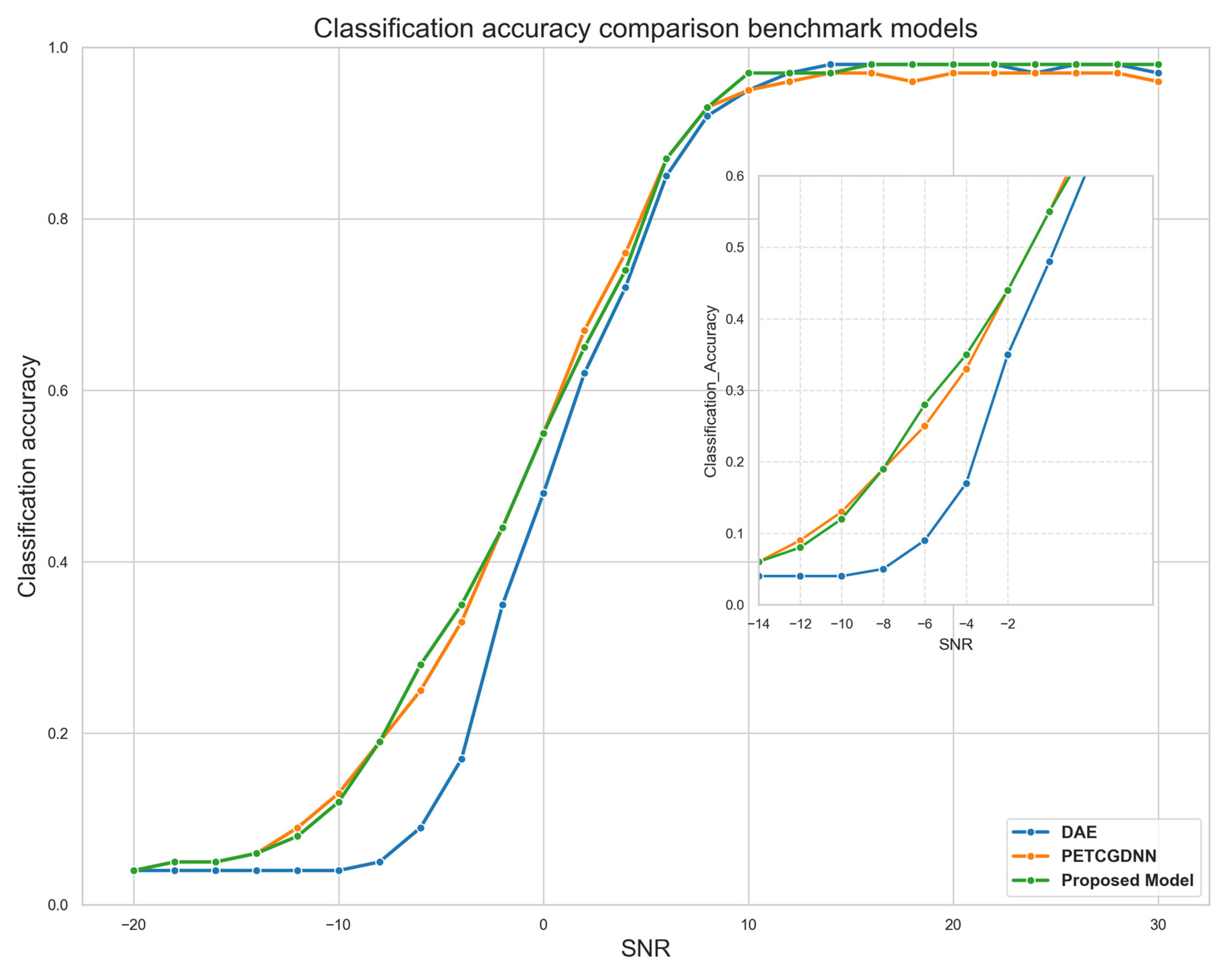
To further evaluate the effectiveness of the proposed model, we compared its classification accuracy across different SNR levels with two representative lightweight baseline models: DAE [7] and PET-CGDNN [17]. As the comparison in Figure 6 shows, the proposed model consistently outperforms DAE at all SNR levels. Notably, under low-SNR conditions (≤0 dB), the performance difference is significant; for example, at −6 dB, the proposed model achieves 27.5% accuracy compared to 9.41% for DAE. When compared to PET-CGDNN, the proposed model shows similar or better performance across the entire SNR range while requiring 3.8 times less computational effort. Although both models follow similar trends above 10 dB, the proposed model has a marked advantage at mid-range SNRs, such as 4 dB and 6 dB. This consistent performance across all SNR conditions—especially in low-SNR environments where signal distortion and noise are more problematic—highlights the robustness and denoising capability of the proposed DP-DRSN with garrote thresholding. These results indicate that the proposed architecture efficiently utilizes its denoising mechanism to deliver high classification accuracy with less energy use and lower latency, which are critical factors in systems with limited computational resources and real-time requirements.

5.4. Ablation Study

The ablation study was conducted to examine how changing the denoising block and feature extraction configurations affects the performance of the proposed model with RML2018.01a datasets. Performance metrics include FLOPs (in millions), memory usage (in GB), inference time (in ms) per sample, energy consumption (in mJ) per sample, and both average and maximum classification accuracy. All models were run under the same run-time conditions using TensorFlow. It is observed that the model’s memory usage remains constant across different configurations because, by default, TensorFlow allocates all available GPU memory. The results of the ablation study are summarized in Table 6.
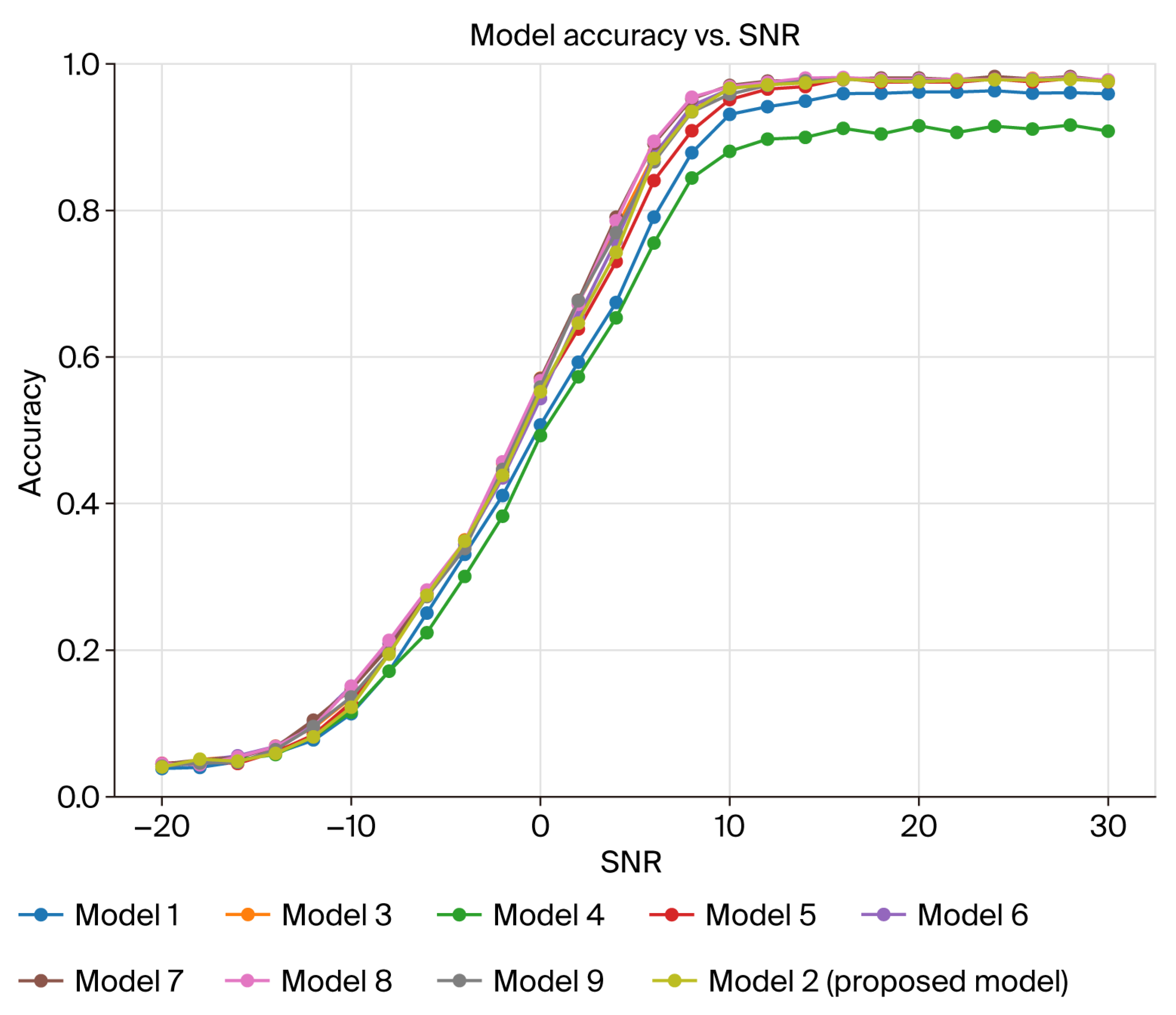
Figure 7 represents a summary of the results from the ablation study of models with varying denoising and feature extraction blocks, showing a comparison of average classification accuracy across all SNR values for each model. First, the impact of increasing the number of DP-DSRN denoising blocks was examined. Model 1, with two blocks, achieved an average accuracy of 59.65% at 11.21 M FLOPs, 0.91 ms of inference time per sample, and 19.21 mJ of energy per sample.
When the number of denoising blocks was increased to four in Model 2, the proposed model improved the average accuracy to 62.13% with a moderate increase in FLOPs to 18.82 M, an inference time of 1.04 ms, and an energy consumption of 31.49 mJ. Furthermore, increasing the number to six blocks in Model 3 resulted in a marginal gain of 62.77% average accuracy, but at a higher computational cost of 30.92 M FLOPs and an energy of 30.71 mJ, without any increase in inference speed. This analysis reveals diminishing returns in accuracy beyond four denoising blocks, accompanied by a significant increase in computation.
Next, the effect of feature extraction was examined. Model 4, which utilized CNN-only extraction, achieved the lowest average accuracy of 56.81% and a maximum accuracy of 91.63%, but was the most efficient, with an inference time of just 0.16 ms and an energy consumption of 4.81 mJ. In contrast, Model 5, which relies solely on LSTM extraction, significantly improves performance, achieving an average accuracy of 61.75% and a maximum of 97.93%, highlighting the benefit of capturing temporal dependencies. However, this came with a higher latency of 1.03 ms and energy use of 28.33 mJ. These findings emphasize the trade-off between effective temporal modeling and computational efficiency.
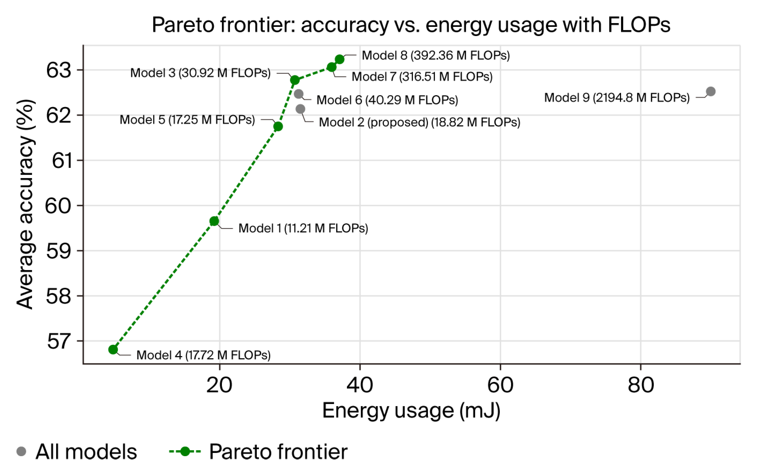
To further analyze performance improvements, tests were conducted by combining LSTM-CNN models with scaled parameters. Note that zero padding was used to match the tensor shape for concatenating CNN and LSTM blocks during feature extraction. Model 6, which increased LSTM units to 8 and CNN filter sizes to 8, maintained an accuracy similar to the proposed model, achieving an average of 62.46% and a maximum classification accuracy of 98.12%. However, it required a higher number of FLOPs (40.29 M) and similar latency. Model 7, further scaled to 16 LSTM units and 16 CNN filter sizes, achieved the highest average accuracy of 63.06% and a maximum accuracy of 98.24%. Still, it required significant computation, including 316.51 M FLOPs, 1.24 ms inference time, and 35.94 mJ of energy. Models 8 and 9 extended this scaling to 6 denoising blocks and larger units/filters of 16 and 32. These models showed minor gains in average accuracy, at 63.23% and 62.52%, but large increases in resource use, especially in FLOPs, reaching 2194.8 M, and energy, up to 90.03 mJ, highlighting a sharp trade-off between performance and efficiency. The Pareto frontier plot shown in Figure 8 illustrates the trade-off between energy consumption and classification accuracy by identifying models that offer the best achievable accuracy for a given energy budget. Notably, the proposed model lies on this frontier, confirming its efficiency and suitability for resource-constrained applications.

6. Discussion, Limitations, and Future Research

6.1. Discussion

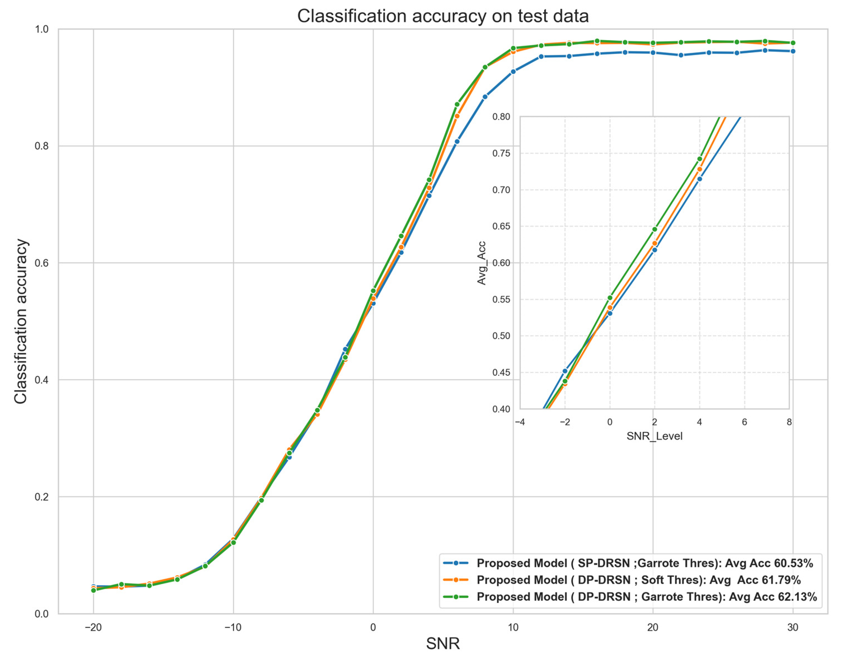
Additional testing was conducted to validate the performance of the SP-DRSN architecture compared to the DP-DRSN architecture, thereby justifying the increased model complexity using DP-DRSN. The SP-DRSN architecture is illustrated in Appendix A.3. In the proposed model, DP-DRSN is replaced by SP-DRSN, utilizing the exact model design shown in Appendix A.1. The average and maximum classification accuracy of SP-DRSN declined by ~1.7% to 60.53% and 96.36%, respectively. However, the tunable parameters of the proposed model with SP-DRSN were reduced to 24,828, i.e., roughly a 9% reduction, and FLOPs were reduced by about 0.6% from 18.82 million to 18.71 million. Figure 9 plots classification accuracy against SNR for a comparison of SP-DRSN vs. DP-DRSN using garrote thresholding. This demonstrates that the proposed model with DP-DRSN balances the demand for classification accuracy and model complexity. The classification accuracy values at each SNR level for the three models are provided in Table 7 for reference.
The proposed model’s performance was also evaluated using the soft thresholding denoising technique instead of the garrote thresholding. With soft thresholding, the overall average classification accuracy declined from 62.13% to 61.79%, and the maximum classification accuracy declined from 97.94% to 97.81% across 24 modulations of RML2018.01a, indicating that the garrote thresholding is slightly better at denoising the radio noise. It is noteworthy that garrote thresholding outperforms soft thresholding at SNR levels ranging from −4 dB to 6 dB, with an average improvement of 2.2%, indicating better performance in a noisy environment at a marginal computational overhead of about 0.6% for FLOPs. A comparison of the performance is shown in Figure 9 with a zoomed-inset plot.
Table 8 shows the results of the statistical paired t-test comparing the classification accuracy for the three models. The results reveal statistically significant differences (p < 0.05) in all model comparisons. Specifically, the proposed DP-DRSN model with garrote thresholding outperformed both the SP-DRSN and DP-DRSN with soft thresholding variants, with p-values of 0.00020 and 0.04601, respectively.

6.2. Limitations

Despite the promising results shown in this study, several limitations should be acknowledged. First, the evaluation of the proposed AMC model depends solely on synthetic datasets (RML2016.10a, RML2016.10b, and RML2018.01a), which, though carefully designed to replicate real-world noisy conditions, may not fully capture the complexities and variations found in actual wireless environments. Real-world testing remains the most reliable method for verifying model robustness and generalizability. Real-world data acquisition and collection are also challenging due to hardware variability, interference, and the complexities involved in a standardized preprocessing pipeline for field-collected data. Second, direct comparisons with state-of-the-art benchmark models are limited due to inconsistencies in training conditions, preprocessing steps, and experimental setups across different studies. A fair and comprehensive benchmark would require all models to be trained, tested, and deployed in a shared and controlled environment. These limitations restrict the conclusiveness of cross-model performance comparisons and emphasize the need for standardized evaluations in AMC research.

6.3. Future Research

As the field of AMC continues to evolve, several promising research avenues merit further exploration to enhance their efficacy and applicability. These focus areas include more efficient signal denoising mechanisms to address the ever-evolving overcrowded wireless spectrum, using real-world data, reducing model energy consumption, reducing FLOPs, and model pruning to reduce model complexity. One of the primary areas for future research is the development of advanced denoising mechanisms. The ongoing expansion of wireless communication systems has created a more crowded spectrum, highlighting the importance of effective signal denoising. Additionally, the current study uses L2 with a regularization factor of 1 × 10⁻⁴ and he_normal initialization to support model generalization and stable training; however, further research is needed on gradient flow within residual denoising paths. Future efforts can address this by performing gradient norm analysis, visualizing gradient flow plots, and conducting a sensitivity analysis of the learnable garrote thresholding parameters γ and κ in (A5) and (A6). These analyses would provide deeper insights into the stability and learnability of the denoising mechanism and its effect on downstream classification performance. Future research should aim to develop innovative denoising algorithms that can accurately filter out noise while preserving essential signal characteristics.
Another critical research direction is the utilization of real-world data to train and test AMC models. Real-world data often presents more complex and diverse scenarios than synthesized data, resulting in a more robust and generalizable model [42]. Future studies should focus on collecting, processing, and leveraging extensive real-world datasets to enhance the performance of AMC systems in practical applications. In addition, a large-scale and stratified sampling approach was used for training, validation, and testing purposes with a fixed random seed to reduce variation in results, but training randomness due to weight initialization and batch ordering can still influence results. Cross-validation can be incorporated in future work to thoroughly capture model randomness.
Improving the energy consumption of AMC models is essential for real-time communication applications. Research efforts should optimize the computational efficiency of these models using techniques such as model compression, hardware acceleration, and algorithmic optimizations, which should be explored to achieve faster inference times and lower energy consumption without compromising recognition accuracy. Another critical area of focus is to reduce the number of FLOPs required by AMC models, which can lead to more efficient models that consume less computational power and energy.
Future research should investigate methods to streamline model architecture, such as employing lightweight neural network designs. Simplifying model architectures with lightweight neural networks, including separable convolutions, complex-value kernels, and sparse self-attention mechanisms, can produce models that are both effective and resource-efficient. These approaches could result in more resource-efficient AMC systems, making them suitable for deployment on edge devices with limited computational capabilities [43]. Model pruning is a valuable technique for reducing the complexity of AMC models. By selectively removing redundant or less significant parameters from the neural network, model pruning can lead to smaller, more efficient models without compromising performance [17]. Future research should focus on developing advanced pruning algorithms that can effectively balance model size and accuracy. The development of more efficient, accurate, and versatile AMC systems ultimately enhances the overall effectiveness of modern communication networks.

7. Conclusions

This study addresses the challenge of deploying deep learning-based AMC models on resource-constrained edge devices by developing a lightweight model that strikes a balance between high classification accuracy and low computational complexity. The proposed model is highly compact, with a size of 108.83 KB and only 27k tunable parameters, and requires 2.36 to 18.82 million FLOPs, achieving inference times between 0.14 and 1.04 ms per sample and an energy consumption of 3.3 to 31.5 mJ per sample. Despite its simplicity, it achieves strong average classification accuracies of 61.20% (RML2016.10a), 63.78% (RML2016.10b), and 62.13% (RML2018.01a), confirming the hypothesis that accurate and efficient AMC is feasible for edge deployment. These results support the model’s suitability for real-world applications, although validation on real-world datasets and standardized benchmarking remain essential next steps to confirm its robustness and generalizability.

Author Contributions

Conceptualization, methodology, formal analysis, writing—original draft preparation, and visualization were performed by P.S. and Y.Q. provided review, editing, and supervision. All authors have read and agreed to the published version of the manuscript.

Funding

This research received no external funding.

Institutional Review Board Statement

Not applicable.

Informed Consent Statement

Not applicable.

Data Availability Statement

Datasets used in this work are provided by DeepSig Inc. and are licensed under the Creative Commons Attribution—NonCommercial—ShareALike 4.0 License (CC BY-NC-SA 4.0); https://www.deepsig.ai/datasets/ (accessed on 5 August 2025).

Acknowledgments

During the preparation of this manuscript/study, the author(s) used Python (3.9.19) and TensorFlow (2.10.1) for the purposes of analysis and visualization creation. The authors have reviewed and edited the output and take full responsibility for the content of this publication.

Conflicts of Interest

The authors declare that they have no conflicts of interest.

Abbreviations

The following abbreviations are used in this manuscript:
AMCAutomatic Modulation Classification
AWGNAdditive White Gaussian Noise
CCECategorical Cross-Entropy
CNNConvolution Neural Network
CRCognitive Radio
CWTContinuous Wavelet Transform
DLDeep Learning
DP-DRSNDual-Path Deep Residual Shrinkage Network
DRSNDeep Residual Shrinkage Network
FLOPsFloating-point Operations per Second
GAPGlobal Average Pooling
GMPGlobal Max Pooling
LSTMLong Short-Term Memory
MSEMean Squared Error
RMLRadio Machine Learning
ReLURectified Linear Unit
SNRSignal-to-Noise Ratio
SP-DRSNSingle-Path Deep Residual Shrinkage Network

Appendix A

Appendix A.1. Model Design
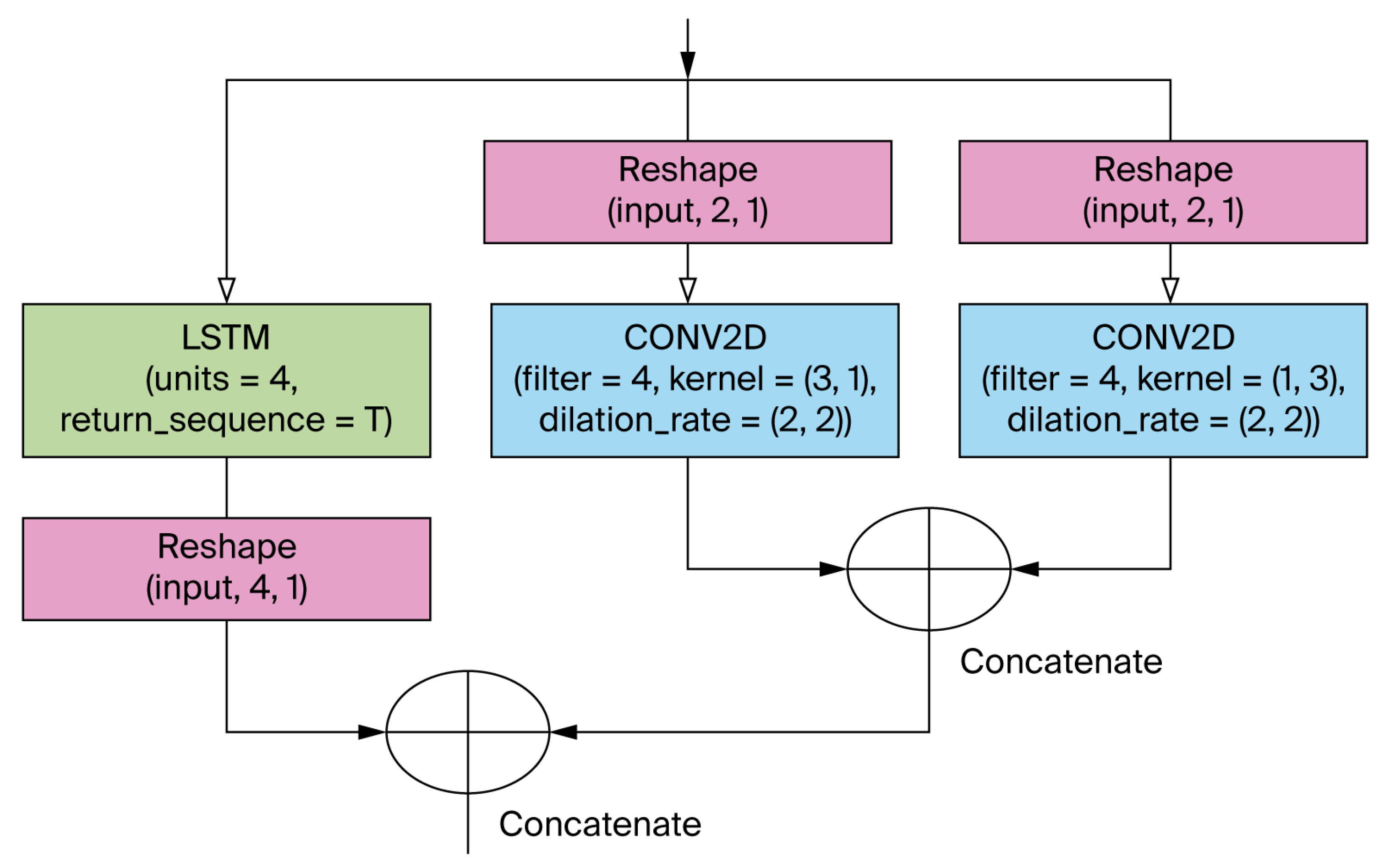
The proposed model has three blocks: feature extraction, denoiser, and classifier. The feature extraction block is a hybrid model composed of LSTM and CNN layers that extract the temporal and spatial features of I/Q and A/P signals (refer to Figure A1). Temporal features are extracted using the LSTM layer with four units while the returning sequence is true. The output of the LSTM layer was reshaped to be concatenated with the CNN block with a filter size of 4. Spatial features were extracted using the asymmetric convolution [19] layers, using a filter size (3 × 1), extracting horizontal features, and (1 × 3) extracting vertical features. This decomposition reduces the number of parameters and speeds up computation. The horizontal and vertical features are concatenated along axis 2. Additionally, the CNN layer employed a dilation factor of (2, 2) to capture global features without incurring a computational cost increase. CNN layers included a kernel initializer of he_normal and the kernel regularizer of L2 with a regularization factor of 1 × 10⁻⁴ to facilitate model convergence. Finally, temporal and spatial features extracted from the LSTM and CNN layers are concatenated along axis 3.
Figure A1. Proposed model feature extraction block.
Ai 06 00195 g0a1
The theory for denoising complex and noisy signals is the continuous wavelet transform (CWT). CWT has been successfully applied for image compression, denoising, and signal processing [44]. In this context, CWT’s ability to denoise the input signal is of prime importance because of its simultaneous time and frequency representation. A time–frequency transform is required in radio signal propagation because the received signal is a non-stationary time series, and a simple Fourier transform is insufficient. CWT is a convolution of the input signal that transforms the input data into a time–frequency representation, facilitating the selection of dynamic thresholds to denoise signals. In a seminal paper, Donoho [45] proposed a thresholding or shrinkage function to denoise noisy signals in the wavelet transform domain. For effective signal denoising in wavelet thresholding, filters must convert useful data into strong features while minimizing noise. Traditional filter design is complex and requires expertise; DL simplifies this by using gradient descent to learn filters automatically. Thus, integrating soft thresholding with DL effectively removes noise and enhances feature discrimination. Zhao et al. [46] modified a residual network [47], a modification of the convolutional neural network (CNN), to alleviate the vanishing gradient issue, called a deep residual shrinkage network (DRSN), to denoise interference signals as input using soft thresholding for fault diagnosis classification of the mechanical transmission system. Within the context of AMC, An et al. [11] used soft thresholding to denoise the I/Q input signal using a hybrid model with CNN and GRU layers.
Salimy et al. [48] extended the work in [46] to develop DP-DRSN as a signal denoising method using a soft thresholding mechanism for fault classification in high-voltage power plant applications. Ruan et al. [49] used DP-DRSN with soft thresholding for side-scan sonar image classification. Inspired by their work, this study uses DP-DRSN for wireless modulated signal classification. We use garrote thresholding instead of soft thresholding because it is designed to address the limitations of the soft threshold method. This technique employs a non-linear approach for values outside its specified threshold parameter range [50]. Values within the threshold range are suppressed to zero, similar to a soft threshold, while values outside range are adjusted to a non-linear shrinkage function, as depicted in (A1). In this expression, x, y i represents the input and output features, respectively, and τ denotes the threshold value.
y i = 0 ,                                                                           x < τ     x τ 2 x + 1 × 10 6 ,               x   τ
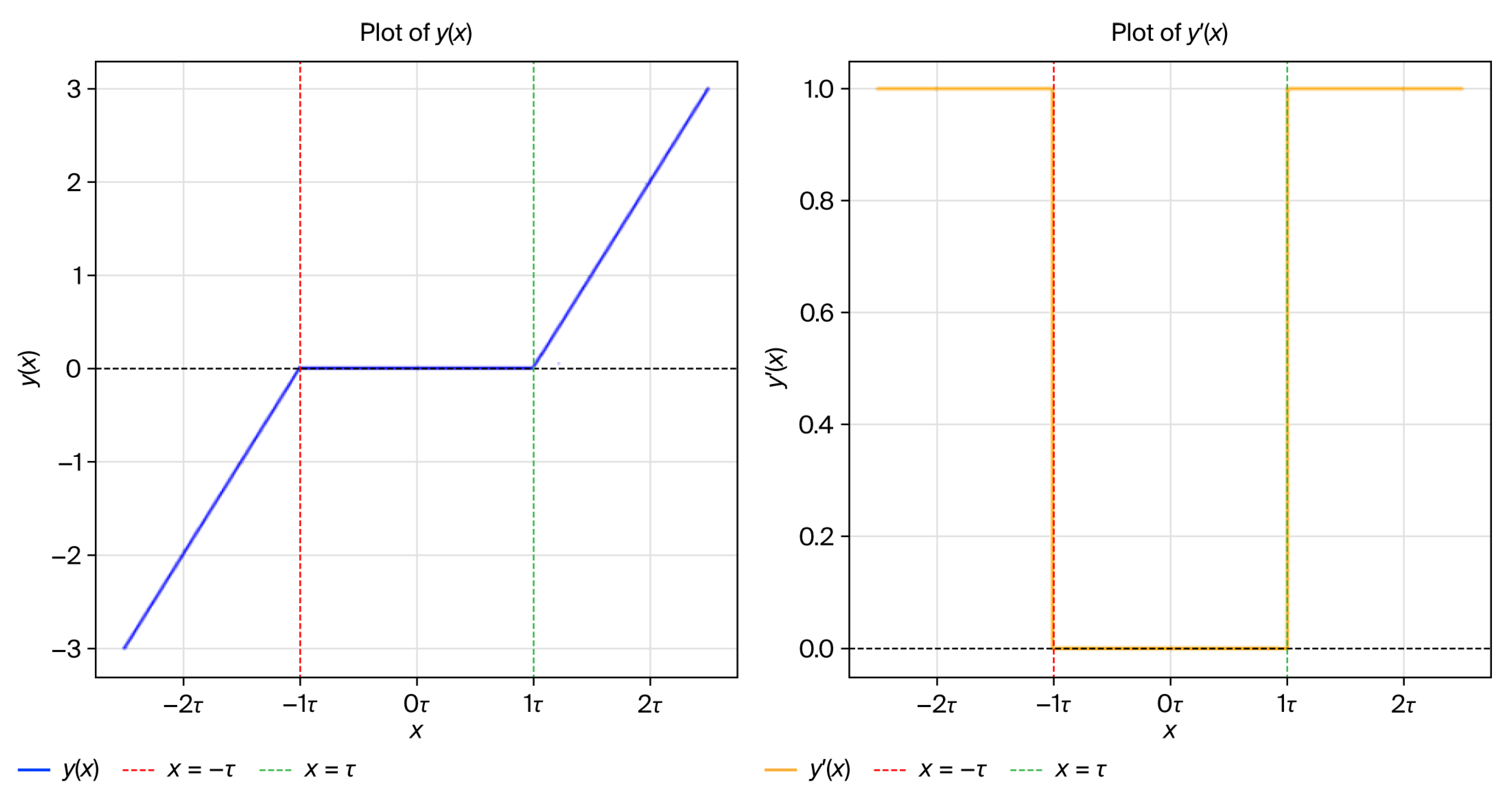
Here, 1 × 10⁻⁶ is a small constant added to the denominator to prevent numerical instability and ensure smooth behavior during gradient computation. The choice of τ > 0 enforces a positive threshold, enabling the model to selectively zero out small-magnitude inputs, preserving or non-linearly attenuating larger activations. The derivative of the garrote function, required for backpropagation, is given in (A2). This derivative is zero within the threshold range and varies non-linearly outside it.
y i = 0 ,                                                                             x < τ   1 + τ 2 x + 1 × 10 6 2 ,               x   τ
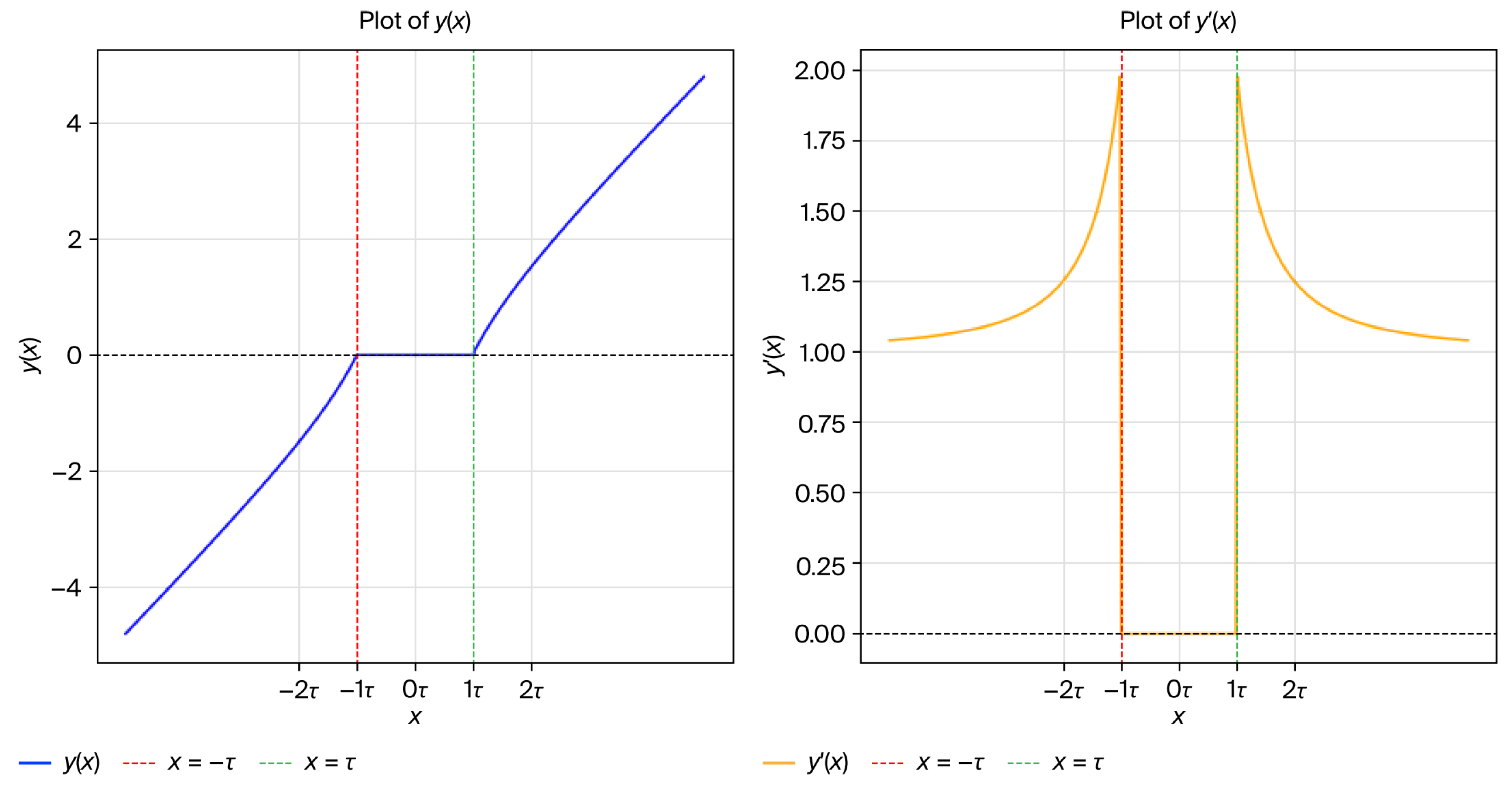
This piecewise-differentiable structure ensures gradient stability during training, avoiding sharp discontinuities that impede convergence. Specifically, the smooth, non-linear nature outside the threshold region promotes stable updates while maintaining sensitivity to informative features with high signal magnitude. This behavior is visually illustrated in Figure A2, which shows how the function suppresses low-magnitude noise while preserving significant signal components. Such a mechanism aligns with non-linear gradient regularization strategies employed in numerical solution of stochastic differential equations and non-linear Kolmogorov partial differential equations [51]. In modulation classification problems, it is crucial to recognize that different modulation types exhibit varying noise levels [52]. Therefore, adjusting the threshold based on the noise level is essential. Prior studies have empirically derived fixed threshold scaling methods for wireless signal denoising [10,44].
In contrast, this paper introduces a self-learnable scaling mechanism integrated into the model optimization process, enabling dynamic adjustment of threshold values during denoising. This approach is particularly critical for real-world applications, where devices encounter highly variable noise conditions in increasingly congested dynamic wireless communication environments.
Figure A2. Garrote thresholding and its derivative.
Ai 06 00195 g0a2
The structure of DP-DRSN using garrote thresholding is shown in Figure A3. DP-DRSN has a subnetwork, which is an intermediate feature mapping x   R C × W × 1 as input. It applies GAP and GMP to the absolute values, extracting the global compressed feature quantity of the current feature map. GAP captures the average contextual representation across all spatial dimensions, enabling the model to understand the overall distribution of signal features. In contrast, GMP isolates the most dominant high-amplitude signal responses, which often correspond to transient peaks or bursts associated with noise or interference. Subsequently, the 1-D vector is fed into two fully connected (FC) layers with batch normalization and rectified linear unit (ReLU) to derive a scaling parameter [53]. A sigmoid function is applied at the end of the two-layer FC network to ensure the scaling parameter falls within the range of (0, 1), as shown below in (A3) and (A4), where α is learned coefficients from z p a t h 1 , which is the output of the two FC layers in the DP-DRSN derived from GAP, and β is learned coefficients from z p a t h 2 , which is the output of the two FC layers in the DP-DRSN derived from GMP.
α = 1 1 + e z p a t h 1
β = 1 1 + e z p a t h 2
Figure A3. Dual-path deep residual shrinkage network (DP-DRSN) architecture.
Ai 06 00195 g0a3
The proposed model determines the threshold by applying auto-scaling τ as shown in (A5) and (A6), where k and γ are self-learning scalar parameters based on the noise level and modulation type. In addition, γ is constrained to the value between 0 and 1. Both values of k and γ are optimized through backpropagation during the training process to minimize the loss function. In addition, the kernel initializer of he_normal and the kernel regularizer of L2 with a regularization factor of 1 × 10⁻⁴ were used for Conv2D and FC layers to improve training convergence.
τ = γ α + 1 γ β , γ = 0,1
T h r e s h o l d = k τ
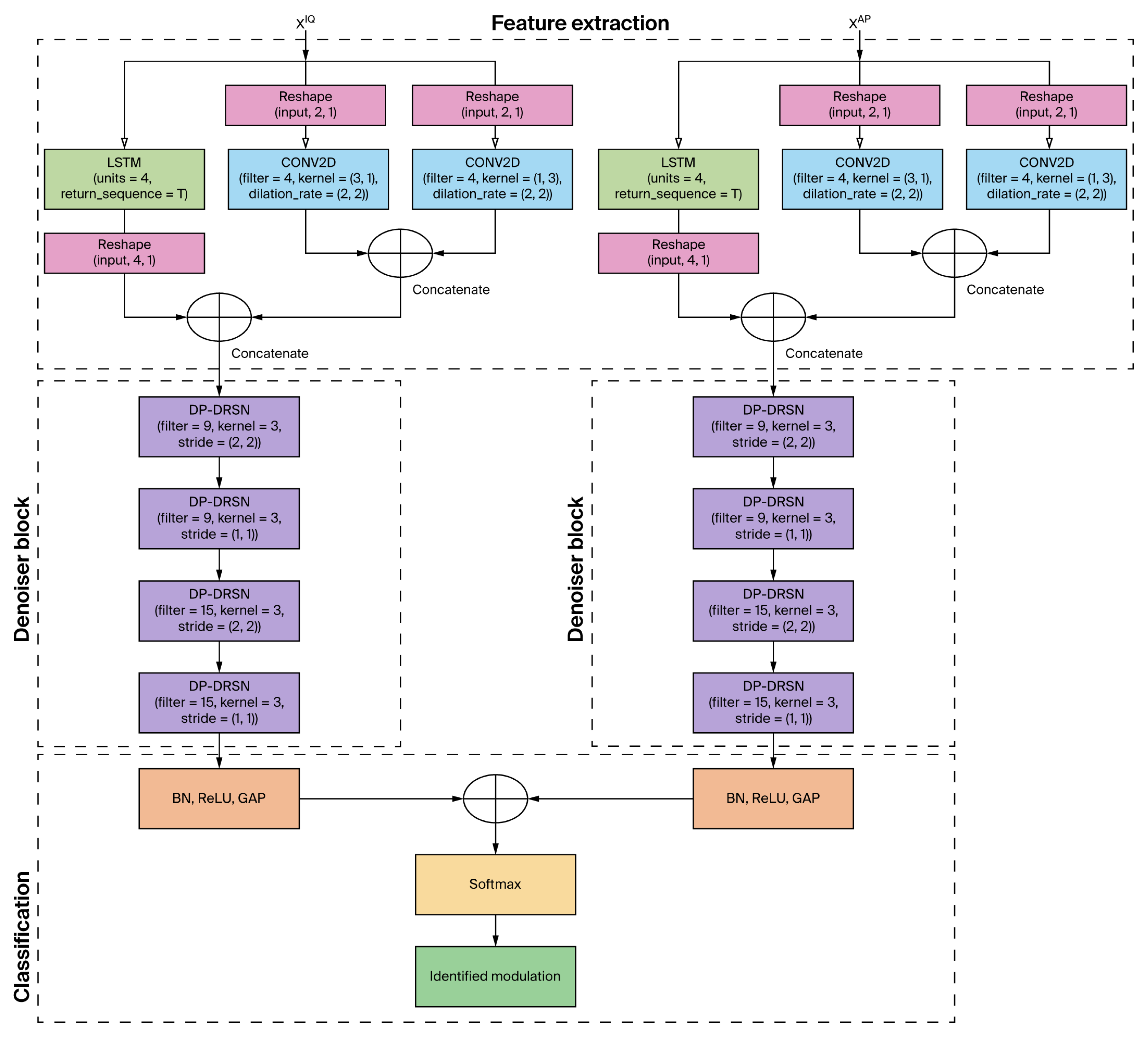
The proposed model’s denoiser block comprises four DP-DRSN layers, which facilitate the learning of discriminative features through various non-linear transformations. Garrote thresholding functions act as shrinkage mechanisms to remove noise-related information, as shown in Figure A4.
Figure A4. Proposed model denoising block—4 layers of DP-DRSN.
Ai 06 00195 g0a4
The Adam optimizer is employed with the categorical cross-entropy (CCE) function as the loss function, shown in (A7), for the optimization process. The classifier block module comprises batch normalization, followed by ReLU and GAP operation before applying SoftMax activation as shown in (A8), where y ^ represents predicted modulation and y represents the ground truth modulation value with x i is i -th AMC output.
L C C E = i N y   l o g ( y ^ )
y ^ = f s o f t m a x ( x i )
Figure A5 shows the complete proposed architecture of the model. The algorithm flow is shown in Table A1. The model takes both I/Q and A/P as input features. The first stage involves extracting spatial and temporal features using CNN and LSTM layers in the feature extraction block for I/Q and A/P inputs. Next, the denoise block minimizes noise features. After that, the denoised I/Q and A/P features are concatenated, and the classifier module identifies modulation classes.
Figure A5. Proposed model architecture.
Ai 06 00195 g0a5
Table A1. Algorithm flow for proposed model using DP-DRSN with garrote thresholding.
  • Inputs:
    Χ I Q , Χ A P ϵ R L X 2
    L : S i g n a l   L e n g t h
    : N u m b e r   o f   m o d u l a t i o n   c l a s s e s
    λ ϵ [ 0,1 ] : L e a r n a b l e   s c a l a r
    κ ϵ R + : L e a r n a b l e   s c a l e r
  • Feature Extraction per Input: Χ ϵ { Χ I Q , Χ A P }
  • LSTM Path: H L S T M = R e s h a p e L S R M 4 Χ ϵ R L x 4 x 1
  • CNN Path:
    Χ r e s h a p e d = R e s h a p e Χ R L x 2 x 1
    F 1 = C o n v 2 D 3 x 1 d i l = 2 Χ r e s h a p e d , F 2 = C o n v 2 D 1 x 3 d i l = 2 ( Χ r e s h a p e d )
    H C N N = C o n c a t a x i s = 2 ( F 1 , F 2 )
  • Combined Feature:
    H i n = C o n c a t a x i s = 3 ( H C N N , H L S T M )
  • Dual Path Residual Shrinkage Block with Self-learning Garrote Denoising
  • Let R 0 = H i n
  • Step1: Residual Path
    R 1 = B N R 0 C o n v 2 D
    R 2 = B N R 1 C o n v 2 D
  • Step 2: Compute Absolute Value A = | R 2 |
  • Step 3: Compute Global Statistics μ = G A P A ϵ R C , υ = G M P A R C
  • Step 4: Calculate the Scaling Coefficient
    α = σ B N D e n s e μ , β = σ B N D e n s e υ
    τ = γ . α + 1 γ . β
    T h r e s h o l d = κ . τ b r o a d c a s t e d   t o   m a t c h   s p a t i a l   s p a c e
  • Step 5: Apply Garrote Thresholding
    Μ s m a l l = I A < T h r e s h o l d , Μ l a r g e = 1 Μ s m a l l
    R s m a l l = Μ s m a l l . 0
    R l a r g e = Μ l a r g e . R 2 T h r e s h o l d 2 R 2 + 1 e 06
    R d e n o i s e d = R s m a l l + R l a r g e
  • Step 6: Skip Connection
    I f   d o w n s a m p l e : Ι = A v g P o o l ( R 0 )
    I f   c h a n n e l R 0 c h a n n e l s R d e n o i s e d : Ι = P a d ( Ι )
    R o u t = R d e n o i s e d + Ι
  • Final Classification:
  • Repeat the above denoising block stack for both IQ and AP paths
  • After final residual shrinkage:
    F I Q = G A P B N R f i n a l I Q , F A P = G A P B N R f i n a l A P
    F c o n c a t = C o n c a t ( F I Q , F A P )
    y ^ = s o f t m a x ( D e s n s e F c o n c a t )

Appendix A.2. Soft Thresholding

Equations (A9) and (A10) illustrate the soft thresholding method and its derivative. It can be seen that soft thresholding removes near-zero values within the threshold range, similarly to garrote thresholding; however, those outside the threshold are adjusted linearly (refer to Figure A6 for soft thresholding and its derivative).
y i =   0 ,                                                                           x < τ x τ . S g n x ,                         x   τ
y i = 0 ,                                                                           x < τ   1 ,                                                                             x   τ
Figure A6. Soft thresholding and its derivative.
Ai 06 00195 g0a6

Appendix A.3. SP-DRSN Architecture

The single-path deep residual shrinkage network (SP-DRSN) has a subnetwork, which is an intermediate feature mapping x    R C × W × 1 as input. It applies only GAP to the absolute values, extracting the global compressed feature quantity of the current feature map. Subsequently, the 1-D vector is fed into two fully connected (FC) layers with batch normalization and rectified linear unit (ReLU) to derive a scaling parameter α , which is then a learning auto-scaling parameter κ . Figure A7 illustrates the SP-DRSN architecture.
Figure A7. Single-path DRSN (SP-DSRN) architecture.
Ai 06 00195 g0a7

References

  1. Zheng, S.; Chen, S.; Qi, P.; Zhou, H.; Yang, X. Spectrum sensing based on deep learning classification for cognitive radios. China Commun. 2020, 17, 138–148. [Google Scholar] [CrossRef]
  2. Zheng, Q.; Tian, X.; Yu, Z.; Wang, H.; Elhanashi, A.; Saponara, S. Dl-pr: Generalized automatic modulation classification method based on deep learning with priori regularization. Eng. Appl. Artif. Intell. 2023, 122, 106082. [Google Scholar] [CrossRef]
  3. Guo, L.; Gao, R.; Cong, Y.; Yang, L. Robust automatic modulation classification under noise mismatch. EURASIP J. Adv. Signal Process. 2023, 2023, 73. [Google Scholar] [CrossRef]
  4. Lin, C.; Zhang, Z.; Wang, L.; Wang, Y.; Zhao, J.; Yang, Z.; Xiao, X. Fast and lightweight automatic modulation recognition using spiking neural network. In Proceedings of the 2024 IEEE International Symposium on Circuits and Systems (ISCAS), Singapore, 19–22 May 2024; pp. 1–5. [Google Scholar] [CrossRef]
  5. O’Shea, T.J.; West, N. Radio machine learning dataset generation with gnu radio. In Proceedings of the GNU Radio Conference, Boulder, CO, USA, 12–16 September 2016; Volume 1. [Google Scholar]
  6. O’Shea, T.J.; Roy, T.; Clancy, T.C. Over-the-air deep learning based radio signal classification. IEEE J. Sel. Top. Signal Process. 2018, 12, 168–179. [Google Scholar] [CrossRef]
  7. Ke, Z.; Vikalo, H. Real-time radio technology and modulation classification via an lstm auto-encoder. IEEE Trans. Wirel. Commun. 2022, 21, 370–382. [Google Scholar] [CrossRef]
  8. Shaik, S.; Kirthiga, S. Automatic modulation classification using densenet. In Proceedings of the 2021 5th International Conference on Computer, Communication and Signal Processing (ICCCSP), Chennai, India, 24–25 May 2021; pp. 301–305. [Google Scholar] [CrossRef]
  9. TianShu, C.; Zhen, H.; Dong, W.; Ruike, L. A iq correlation and long-term features neural network classifier for automatic modulation classification. In Proceedings of the 2022 IEEE 10th International Conference on Information, Communication and Networks (ICICN), Zhangye, China, 23–24 August 2022; pp. 396–400. [Google Scholar] [CrossRef]
  10. Shen, Y.; Yuan, H.; Zhang, P.; Li, Y.; Cai, M.; Li, J. A multi-subsampling self-attention network for unmanned aerial vehicle-to-ground automatic modulation recognition system. Drones 2023, 7, 376. [Google Scholar] [CrossRef]
  11. An, T.T.; Puspitasari, A.A.; Lee, B.M. Efficient automatic modulation classification for next generation wireless networks. TechRxiv 2023. [Google Scholar] [CrossRef]
  12. Gao, M.; Tang, X.; Pan, X.; Ren, Y.; Zhang, B.; Dai, J. Modulation recognition of communication signal with class-imbalance sample based on cnn-lstm dual channel model. In Proceedings of the 2023 IEEE International Conference on Signal Processing, Communications and Computing (ICSPCC), Zhengzhou, China, 14–17 November 2023; pp. 1–6. [Google Scholar] [CrossRef]
  13. Ren, Y.; Tang, X.; Zhang, B.; Feng, J.; Gao, M. Modulation Recognition Method of Communication Signal Based on CNN-LSTM Dual Channel. In Proceedings of the 2022 5th International Conference on Information Communication and Signal Processing (ICICSP), Shenzhen, China, 16–18 September 2022; pp. 133–137. [Google Scholar] [CrossRef]
  14. Li, W.; Deng, W.; Wang, K.; You, L.; Huang, Z. A complex-valued transformer for automatic modulation recognition. IEEE Internet Things J. 2024, 11, 22197–22207. [Google Scholar] [CrossRef]
  15. Su, H.; Fan, X.; Liu, H. Robust and efficient modulation recognition with pyramid signal transformer. In Proceedings of the GLOBECOM 2022–2022 IEEE Global Communications Conference, Rio de Janeiro, Brazil, 4–8 December 2022; pp. 1868–1874. [Google Scholar] [CrossRef]
  16. Ding, R.; Zhou, F.; Wu, Q.; Dong, C.; Han, Z.; Dobre, O.A. Data and knowledge dual-driven automatic modulation classification for 6g wireless communications. IEEE Trans. Wirel. Commun. 2023, 23, 4228–4242. [Google Scholar] [CrossRef]
  17. Zhang, F.; Luo, C.; Xu, J.; Luo, Y. An efficient deep learning model for automatic modulation recognition based on parameter estimation and transformation. IEEE Commun. Lett. 2021, 25, 3287–3290. [Google Scholar] [CrossRef]
  18. Guo, W.; Yang, K.; Stratigopoulos, H.-G.; Aboushady, H.; Salama, K.N. An end-to-end neuromorphic radio classification system with an efficient sigma-delta-based spike encoding scheme. IEEE Trans. Artif. Intell. 2024, 5, 1869–1881. [Google Scholar] [CrossRef]
  19. Li, Z.; Zhang, W.; Wang, Y.; Li, S.; Sun, X. A lightweight multi-feature fusion structure for automatic modulation classification. Phys. Commun. 2023, 61, 102170. [Google Scholar] [CrossRef]
  20. Zheng, Y.; Ma, Y.; Tian, C. Tmrn-glu: A transformer-based automatic classification recognition network improved by gate linear unit. Electronics 2022, 11, 1554. [Google Scholar] [CrossRef]
  21. Ning, M.; Zhou, F.; Wang, W.; Wang, Y.; Fei, S.; Wang, J. Automatic modulation recognition method based on multimodal i/q-frft fusion. Preprints 2024. [Google Scholar] [CrossRef]
  22. Shi, F.; Hu, Z.; Yue, C.; Shen, Z. Combining neural networks for modulation recognition. Digit. Signal Process. 2022, 120, 103264. [Google Scholar] [CrossRef]
  23. Xue, M.L.; Huang, M.; Yang, J.J.; Wu, J.D. Mlresnet: An efficient method for automatic modulation classification based on residual neural network. In Proceedings of the 2021 2nd International Symposium on Computer Engineering and Intelligent Communications (ISCEIC), Nanjing, China, 6–8 August 2021; pp. 122–126. [Google Scholar] [CrossRef]
  24. Riddhi, S.; Parmar, A.; Captain, K.; Ka, D.; Chouhan, A.; Patel, J. A dual-stream convolution-gru-attention network for automatic modulation classification. In Proceedings of the 2024 16th International Conference on COMmunication Systems & NETworkS (COMSNETS), Bengaluru, India, 3–7 January 2024; pp. 720–724. [Google Scholar] [CrossRef]
  25. Parmar, A.; Ka, D.; Chouhan, A.; Captain, K. Dual-stream cnn-bilstm model with attention layer for automatic modulation classification. In Proceedings of the 2023 15th International Conference on COMmunication Systems & NETworkS (COMSNETS), Bangalore, India, 3–8 January 2023; pp. 603–608. [Google Scholar] [CrossRef]
  26. Parmar, A.; Chouhan, A.; Captain, K.; Patel, J. Deep multilevel architecture for automatic modulation classification. Phys. Commun. 2024, 64, 102361. [Google Scholar] [CrossRef]
  27. Chang, S.; Yang, Z.; He, J.; Li, R.; Huang, S.; Feng, Z. A fast multi-loss learning deep neural network for automatic modulation classification. IEEE Trans. Cogn. Commun. Netw. 2023, 9, 1503–1518. [Google Scholar] [CrossRef]
  28. Chang, S.; Huang, S.; Zhang, R.; Feng, Z.; Liu, L. Multitask-learning-based deep neural network for automatic modulation classification. IEEE Internet Things J. 2022, 9, 2192–2206. [Google Scholar] [CrossRef]
  29. Luo, Z.; Xiao, W.; Zhang, X.; Zhu, L.; Xiong, X. Rlitnn: A multi-channel modulation recognition model combining multi-modal features. IEEE Trans. Wirel. Commun. 2024, 23, 19083–19097. [Google Scholar] [CrossRef]
  30. Harper, C.; Thornton, M.A.; Larson, E.C. Learnable statistical moments pooling for automatic modulation classification. In Proceedings of the ICASSP 2024—2024 IEEE International Conference on Acoustics, Speech and Signal Processing (ICASSP), Seoul, Republic of Korea, 14–19 April 2024; pp. 8981–8985. [Google Scholar] [CrossRef]
  31. Harper, C.A.; Thornton, M.A.; Larson, E.C. Automatic modulation classification with deep neural networks. Electronics 2023, 12, 3962. [Google Scholar] [CrossRef]
  32. Huynh-The, T.; Hua, C.-H.; Pham, Q.-V.; Kim, D.-S. Mcnet: An efficient cnn architecture for robust automatic modulation classification. IEEE Commun. Lett. 2020, 24, 811–815. [Google Scholar] [CrossRef]
  33. Sun, S.; Wang, Y. A novel deep learning automatic modulation classifier with fusion of multichannel information using gru. EURASIP J. Wirel. Commun. Netw. 2023, 2023, 66. [Google Scholar] [CrossRef]
  34. Nisar, M.Z.; Ibrahim, M.S.; Usman, M.; Jeong-A, L. A lightweight deep learning model for automatic modulation classification using residual learning and squeeze–excitation blocks. Appl. Sci. 2023, 13, 5145. [Google Scholar] [CrossRef]
  35. Nguyen, T.-V.; Nguyen, T.T.; Ruby, R.; Zeng, M.; Kim, D.-S. Automatic modulation classification: A deep architecture survey. IEEE Access 2021, 9, 142950–142971. [Google Scholar] [CrossRef]
  36. Luo, R.; Sun, J.; Guo, Y. Deep learning-based modulation recognition for imbalanced classification. In Proceedings of the 2023 4th International Conference on Machine Learning and Computer Application, Association for Computing Machinery, Hangzhou, China, 27–29 October 2023; pp. 531–535. [Google Scholar] [CrossRef]
  37. Tekbıyık, K.; Ekti, A.R.; Görçin, A.; Kurt, G.K.; Keçeci, C. Robust and fast automatic modulation classification with cnn under multipath fading channels. In Proceedings of the 2020 IEEE 91st Vehicular Technology Conference (VTC2020-Spring), Antwerp, Belgium, 25–28 May 2020; pp. 1–6. [Google Scholar] [CrossRef]
  38. Cheng, R.; Chen, Q.; Huang, M. Automatic modulation recognition using deep cvcnn-lstm architecture. Alex. Eng. J. 2024, 104, 162–170. [Google Scholar] [CrossRef]
  39. Rajendran, S.; Meert, W.; Giustiniano, D.; Lenders, V.; Pollin, S. Deep learning models for wireless signal classification with distributed low-cost spectrum sensors. IEEE Trans. Cogn. Commun. Netw. 2018, 4, 433–445. [Google Scholar] [CrossRef]
  40. Xu, J.; Luo, C.; Parr, G.; Luo, Y. A Spatiotemporal Multi-Channel Learning Framework for Automatic Modulation Recognition. IEEE Wirel. Commun. Lett. 2020, 9, 1629–1632. [Google Scholar] [CrossRef]
  41. Xiao, C.; Yang, S.; Feng, Z. Complex-valued depthwise separable convolutional neural network for automatic modulation classification. IEEE Trans. Instrum. Meas. 2023, 72, 1–10. [Google Scholar] [CrossRef]
  42. Syed, S.N.; Lazaridis, P.I.; Khan, F.A.; Ahmed, Q.Z.; Hafeez, M.; Ivanov, A.; Poulkov, V.; Zaharis, Z.D. Deep neural networks for spectrum sensing: A review. IEEE Access 2023, 11, 89591–89615. [Google Scholar] [CrossRef]
  43. Zhang, F.; Luo, C.; Xu, J.; Luo, Y.; Zheng, F.-C. Deep learning based automatic modulation recognition: Models, datasets, and challenges. Digit. Signal Process. 2022, 129, 103650. [Google Scholar] [CrossRef]
  44. Chen, G.; Xie, W.; Zhao, Y. Wavelet-based denoising: A brief review. In Proceedings of the 2013 Fourth International Conference on Intelligent Control and Information Processing (ICICIP), Beijing, China, 9–11 June 2013; pp. 570–574. [Google Scholar] [CrossRef]
  45. Donoho, D.L. De-noising by soft-thresholding. IEEE Trans. Inf. Theory 1995, 41, 613–627. [Google Scholar] [CrossRef]
  46. Zhao, M.; Zhong, S.; Fu, X.; Tang, B.; Pecht, M. Deep residual shrinkage networks for fault diagnosis. IEEE Trans. Ind. Inform. 2020, 16, 4681–4690. [Google Scholar] [CrossRef]
  47. He, K.; Zhang, X.; Ren, S.; Sun, J. Deep residual learning for image recognition. In Proceedings of the IEEE Conference on Computer Vision and Pattern Recognition, Las Vegas, NV, USA, 27–30 June 2016; pp. 770–778. [Google Scholar] [CrossRef]
  48. Salimy, A.; Mitiche, I.; Boreham, P.; Nesbitt, A.; Morison, G. Dynamic Noise Reduction with Deep Residual Shrinkage Networks for Online Fault Classification. Sensors 2022, 22, 515. [Google Scholar] [CrossRef] [PubMed]
  49. Ruan, F.; Dang, L.; Ge, Q.; Zhang, Q.; Qiao, B.; Zuo, X. Dual-path residual “shrinkage” network for side-scan sonar image classification. Comput. Intell. Neurosci. 2022, 2022, 6962838. [Google Scholar] [CrossRef]
  50. Gao, H.-Y. Wavelet shrinkage denoising using the non-negative garrote. J. Comput. Graph. Stat. 1998, 7, 469–488. [Google Scholar] [CrossRef]
  51. Marino, R.; Macris, N. Solving non-linear kolmogorov equations in large dimensions by using deep learning: A numerical comparison of discretization schemes. J. Sci. Comput. 2023, 94, 8. [Google Scholar] [CrossRef]
  52. An, T.T.; Lee, B.M. Robust automatic modulation classification in low signal to noise ratio. IEEE Access 2023, 11, 7860–7872. [Google Scholar] [CrossRef]
  53. Hu, J.; Shen, L.; Sun, G. Squeeze-and-excitation networks. In Proceedings of the IEEE Conference on Computer Vision and Pattern Recognition, Salt Lake City, UT, USA, 18–23 June 2018; pp. 7132–7141. [Google Scholar]
Figure 1. Proposed model training and validation loss for RML2016.10a, RML2016.10b, and RML2018.01a dataset.
Ai 06 00195 g001
Figure 2. Proposed model classification accuracy at each SNR level for RML2016.10a, RML2016.10b, and RML2018.01a dataset.
Ai 06 00195 g002
Figure 3. Confusion matrix at 0 dB SNR for RML2016.10a, RML2016.10b, and RML2018.01a.
Ai 06 00195 g003
Figure 4. Confusion matrix at 18 dB SNR for RML2016.01a and RML2016.10b, and at 30 dB SNR for RML2018.01a.
Ai 06 00195 g004
Figure 5. Average classification accuracy vs. FLOPs for benchmark models.
Ai 06 00195 g005
Figure 6. Comparison of classification accuracy between DAE, PET-CGDNN, and proposed model at each SNR level.
Ai 06 00195 g006
Figure 7. Comparison of classification accuracy for all nine models at each SNR level, based on the ablation study results in Table 6.
Ai 06 00195 g007
Figure 8. Pareto frontier chart classification accuracy vs. energy usage per test sample for models in ablation study.
Ai 06 00195 g008
Figure 9. Proposed model classification accuracy vs. SNR for SP-DRSN garrote thresholding, DP-DRSN garrote thresholding, and DP-DRSN with soft thresholding.
Ai 06 00195 g009
Table 1. Model performance by tunable parameters. Datasets: A: RML2016.10a; B: RML2016.10b; C: RML2018.01a.
AuthorYearModel NameDL ArchitectureTrainable
Parameters
DatasetAvg
Accuracy
Max
Accuracy
Lin et al. [4]2024 LSM7kA36.39%
B39.74%
C53.79%
Ke and Vikalo [7]2022DAELSTM14kC58.74%97.91%
Shaik and Kirthiga [8]2021 DenseNet19kC55%
TianShu et al. [9]2022IQCLNetCNN, LSTM29kA59.73%
Shen et al. [10]2023MSSACNN36k to 218kC55.25% to 60.90%
An et al. [11]2023TDRNNCNN, GRU41kA63.5%
[−8 dB to18 dB]
Gao et al. [12]2023 CNN, LSTM43kA66.7%
[5 Modulations]
Li et al. [14]2024CV-TRNComplex-Value Transformer44kA63.74%93.76%
C64.13%98.95%
Su et al. [15]2022SigFormerTransformer44kA63.71%93.60%
44kB65.77%94.80%
158kC63.96%97.50%
Ding et al. [16]2023 CNN, BiGRU69kC 34% (−10 dB)
[−10 dB to 2 dB]
Zhang et al. [17]2021PET-CGDNNCNN, GRU71k to 75kA60.44%
B63.82%
C63.00%
Guo et al. [18]2024 SNN84k–627k,
83k–542k
A56.69%
C64.29%
Li et al. [19]2023LightMFFSCNN95kA63.44%
B65.44%
Zheng et al. [20]2022TMRN-GLU (small/large)Transformer25k (Small)
106k (Large)
B61.7% (Small)
65.7% (Large)
93.70%
Ning et al. [21]2024MAMRTransformer110kB61.50%
Shi et al. [22]2022 CNN, SE block113kC 98.70%
Xue et al. [23]2021MLResNetCNN, LSTM115kC 96.6% (18 dB)
Riddhi et al. [24]2024 CNN, GRU145kB68.23%
[Digital Mod]
Parmar et al. [25]2023 CNN, BiLSTM146kB68.23%
Parmar et al. [26]2024 CNN, LSTM155kB63%
Chang et al. [27]2023FastMLDNNCNN, Transformer159kA63.24%
Luo et al. [29]2024RLITNNCNN, LSTM, Transformer181kA63.84%
B65.32%
Harper et al. [30]2024 CNN, SE Block200kC63.15%
Harper et al. [31]2023 CNN, SE Block203kC63.70%98.90%
Huynh-The et al. [32]2020MCNetCNN220kC 93% (20 dB)
Sun & Wang [33]2023FGDNNCNN, GRU253kC 90% (8 dB)
Nisar et al. [34]2023 CNN, SE Block253kA 81% (18 dB)
Proposed Model CNN, LSTM, DP-DRSN27kA61.20%91.23%
B63.78%93.64%
C62.13%97.94%
Table 2. Dataset with training, validation, and testing configuration.
DatasetSignal
Dimension
SNR RangeTrain/
Validation/
Test Sample Size
Modulation Classes
RML2016.10a2 × 128−20 dB to 18 dB132k/44k/44k11
RML2016.10b2 × 128−20 dB to 18 dB720k/240k/240k10
RML2018.01a2 × 1024−20 dB to 30 dB1M/200k/200k24
Table 3. Proposed model training parameters, FLOPs, and classification accuracy.
DatasetTrainable ParameterFLOPsAvg
Acc.
Max.
Acc.
RML2016.10a26,6382.36 M61.20%91.23%
RML2016.10b26,6382.36 M63.78%93.64%
RML2018.01a27,07218.82 M62.13%97.94%
Table 4. Proposed model memory usage, inference time/sample, and energy usage.
DatasetMemory Usage (GB)Inference Time/Sample
(ms)
Energy Usage/Sample
(mJ)
RML2016.10a10.470.143.31
RML2016.10b10.580.253.85
RML2018.01a10.581.0431.49
Table 5. Performance against benchmark models for the RML2018.01a dataset.
ModelAvg. Acc.Max. Acc.FLOPs
(M)
Inference Time/Sample (ms)Param.
(K)
ResNet [6]59.29%94.12%12.185.40163.22
DAE [7]58.74%98.91%2.890.4314.88
LSTM [39]61.78%97.92%206.638.52202.78
MCLDNN [40]61.08%96.84%443.3642.41427.88
PET-CGDNN [17]61.76%96.93%71.9220.6375.34
CDSCNN [41]62.52%98.01%74.116.80322.62
CV-TRN [14]64.13%98.85%6.426.8144.79
Proposed Model62.13%97.94%18.821.0427.07
Table 6. Summary of results from ablation study of models with varying denoising and feature extraction blocks.
Feature ExtractionDenoising Blocks (Garrote Thresholding)Model Performance Results
ModelLSTMCNNDP-DRSN BlocksDenoising ParametersTrainable ParamFLOPs (M)Memory Usage
(GB)
Inference Time (ms)Energy Usage (mJ)Avg Acc.Max Acc.
Denoising Block Size 2, 4, 6
Model 1Unit = 4Filter = 42Filter = 9, Stride = (2, 2);
Filter = 9, Stride = (1, 1);
775611.2110.580.9119.2159.65%96.12%
Model 2 (Proposed Model)Unit = 4Filter = 44Filter = 9, Stride = (2, 2);
Filter = 9, Stride = (1, 1);
Filter = 15, Stride = (2, 2);
Filter = 15, Stride = (1, 1)
27,07218.8210.581.0431.4962.13%97.94%
Model 3Unit = 4Filter = 46Filter = 9, Stride = (2, 2);
Filter = 9, Stride = (1, 1);
Filter = 15, Stride = (2, 2);
Filter = 15, Stride = (1, 1);
Filter = 27, Stride = (2, 2);
Filter = 27, Stride = (1, 1)
87,48830.9210.581.0430.7162.77%98.24%
Feature Extraction: LSTM only and CNN only
Model 4XFilter = 44Filter = 9, Stride = (2, 2);
Filter = 9, Stride = (1, 1);
Filter = 15, Stride = (2, 2);
Filter = 15, Stride = (1, 1)
27,51217.7210.470.164.8156.81%91.63%
Model 5Unit = 4X4Filter = 9, Stride = (2, 2);
Filter = 9, Stride = (1, 1);
Filter = 15, Stride = (2, 2);
Filter = 15, Stride = (1, 1)
26,34417.2510.581.0328.3361.75%97.93%
Feature Extraction: increasing LSTM unit, CNN Filter Size, and Denoising Blocks
Model 6Unit = 8Filter = 84Filter = 9, Stride = (2, 2);
Filter = 9, Stride = (1, 1);
Filter = 15, Stride = (2, 2);
Filter = 15, Stride = (1, 1)
28,28040.2910.581.0531.2362.46%98.12%
Model 7Unit = 16Filter = 164Filter = 17, Stride = (2, 2);
Filter = 17, Stride = (1, 1);
Filter = 33, Stride = (2, 2);
Filter = 33, Stride = (1, 1)
118,940316.5110.581.2435.9463.06%98.24%
Model 8Unit = 16Filter = 166Filter = 17, Stride = (2, 2);
Filter = 17, Stride = (1, 1);
Filter = 33, Stride = (2, 2);
Filter = 33, Stride = (1, 1);
Filter = 47, Stride = (2, 2);
Filter = 47, Stride = (1, 1)
304,800392.3610.581.2237.0763.23%98.24%
Model 9Unit = 32Filter = 326Filter = 33, Stride = (2, 2);
Filter = 33, Stride = (1, 1);
Filter = 47, Stride = (2, 2);
Filter = 47, Stride = (1, 1);
Filter = 65, Stride = (2, 2);
Filter = 65, Stride = (1, 1)
650,0122194.810.583.2190.0362.52%98.03%
Table 7. Classification accuracy at each SNR for SP-DRSN (garrote thres.), DP-DRSN (garrote thres.), and SP-DRSN (soft thres.) models.
SNR Levels
Model−20−18−16−14−12−10−8−6−4−2024
SP-DRSN; Garrote Thres: Avg Acc 60.53%4.68%4.63%4.81%5.96%8.40%12.82%19.88%26.78%34.41%45.21%53.08%61.76%71.47%
DP-DRSN; Soft Thres: Avg Acc 61.79%4.37%4.53%5.16%6.22%8.06%12.69%19.79%28.07%34.07%43.45%53.87%62.68%72.81%
DP-DRSN; Garrote Thres: Avg Acc 62.13%4.00%5.07%4.81%5.88%8.15%12.19%19.41%27.50%34.80%43.83%55.23%64.59%74.22%
Model681012141618202224262830
SP-DRSN; Garrote Thres: Avg Acc 60.53%80.76%88.41%92.70%95.29%95.36%95.76%96.01%95.95%95.51%95.95%95.92%96.36%96.19%
DP-DRSN; Soft Thres: Avg Acc 61.79%85.11%93.48%96.09%97.31%97.62%97.57%97.62%97.34%97.66%97.74%97.81%97.49%97.66%
DP-DRSN; Garrote Thres: Avg Acc 62.13%87.10%93.47%96.71%97.17%97.40%97.95%97.74%97.62%97.73%97.86%97.79%97.94%97.61%
Table 8. Result of paired t-test for SPRDRSN garrote thresholding, DP-DSRN garrote thresholding, and DP-DRSN soft thresholding.
Comparisont-Statisticp-ValueSignificance
(Alpha = 0.05)
SP-DRSN (Garrote Thres) vs. DP-DRSN (Soft Thres)−4.20.0003Significant
SP-DRSN (Garrote Thres) vs. DP-DRSN (Garrote Thres)−4.350.0002Significant
DP-DRSN (Soft Thres) vs. DP-DRSN (Garrote Thres)−2.10.046Significant
Disclaimer/Publisher’s Note: The statements, opinions and data contained in all publications are solely those of the individual author(s) and contributor(s) and not of MDPI and/or the editor(s). MDPI and/or the editor(s) disclaim responsibility for any injury to people or property resulting from any ideas, methods, instructions or products referred to in the content.