
OLTEM: Lumped Thermal and Deep Neural Model for PMSM Temperature

 ,
,
Abstract
1. Introduction
2. Research Object and Modeling
2.1. Research Object
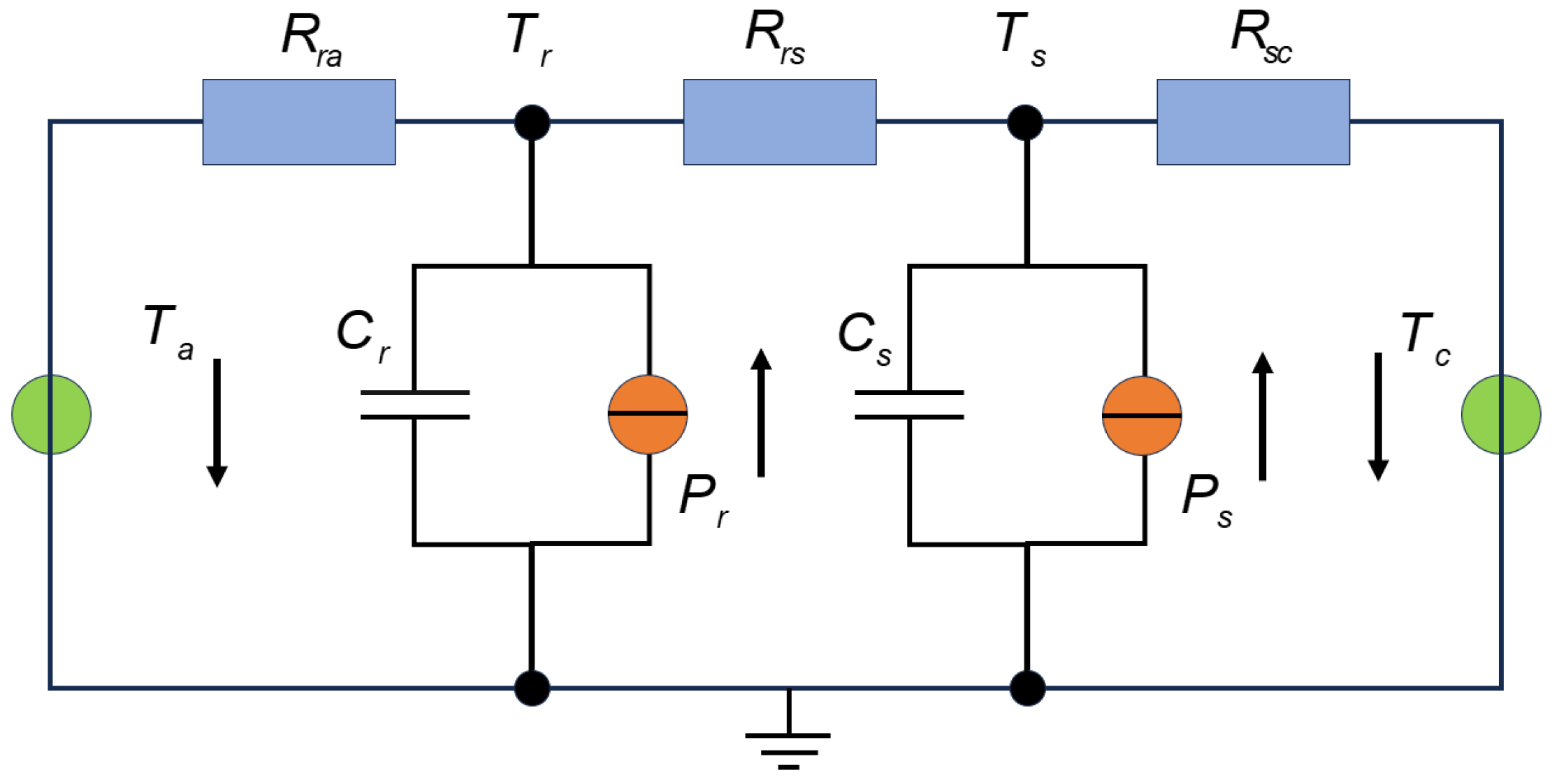
2.2. Traditional LPTN and Its Limitations
3. Methodology
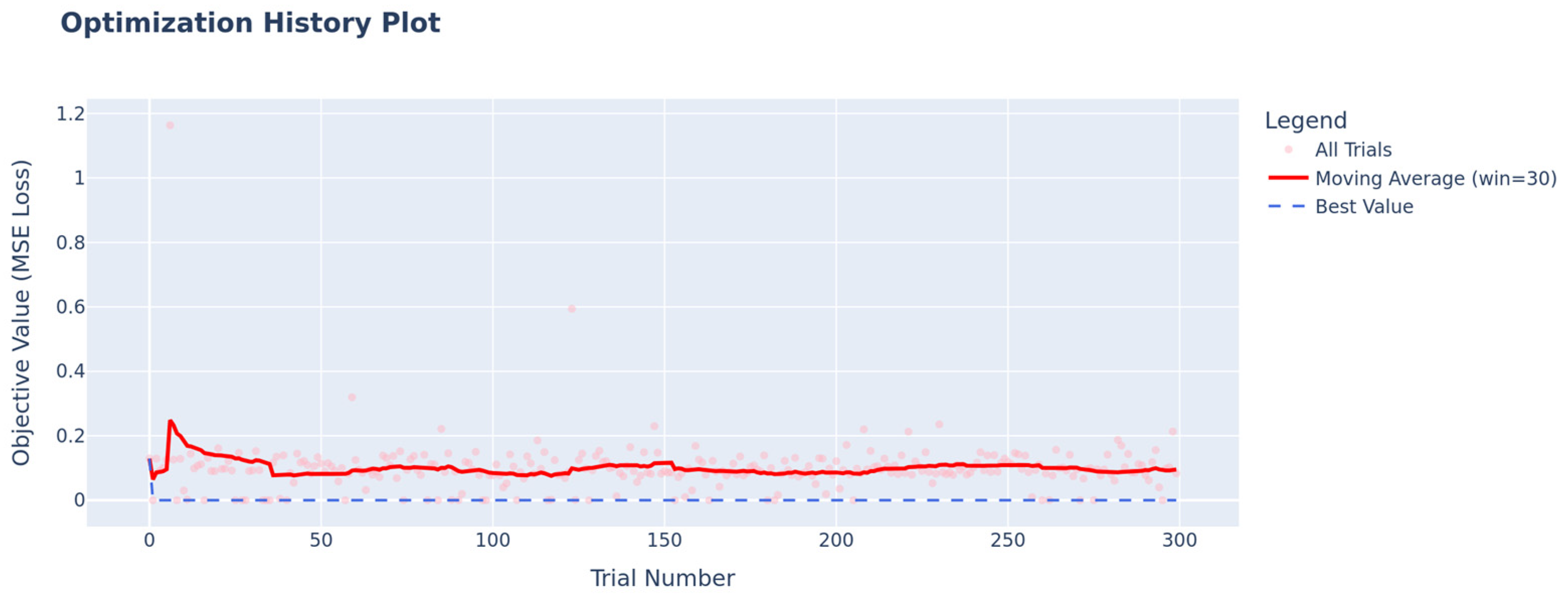
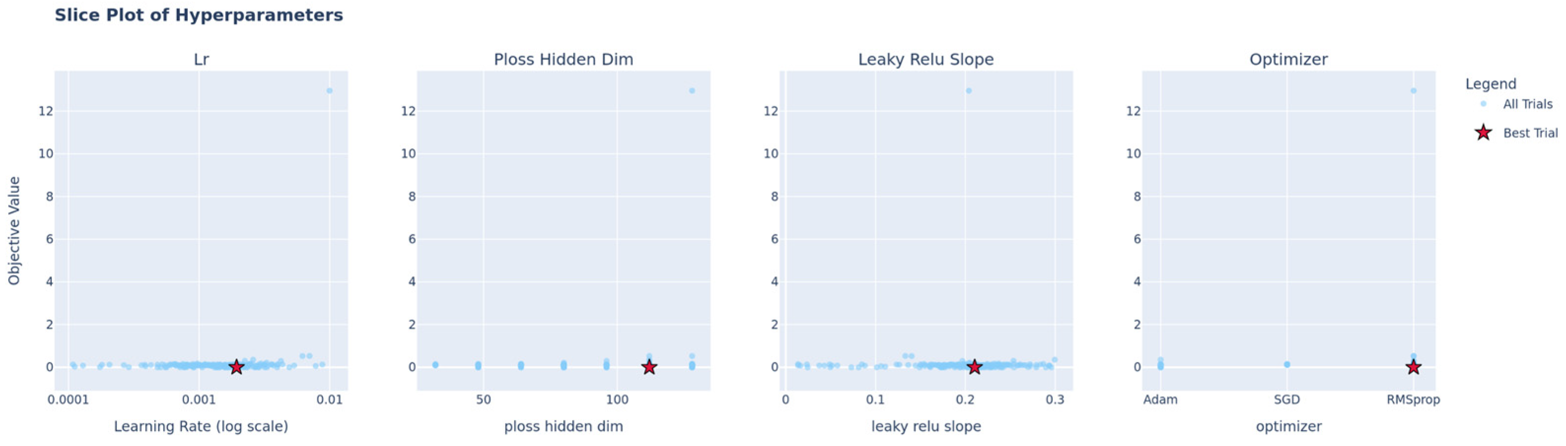
3.1. Hyperparameter Optimization
- Learning Rate (lr): A log-uniform distribution between 1 × 10⁻⁴ and 1 × 10⁻².
- Optimizer: A categorical choice from [‘Adam’, ‘RMSprop’, ‘SGD’].
- Hidden Dimension of Power Loss Net (ploss_hidden_dim): An integer value between 64 and 128.
- Slope of Leaky ReLU (leaky_relu_slope): A uniform distribution between 0.01 and 0.3.
3.2. Baseline Thermal Neural Network (TNN) Architecture
- (1)
- Thermal Capacitance Estimation Network: Corresponding to the parameter in Equation (3), this network is responsible for modeling the inverse thermal capacitance using end-to-end trainable constants.
- (2)
- Thermal Conductivity and Power Dissipation Estimation Network: Corresponding to parameters and in Equation (3), this sub-network processes the input measurement data and temperature estimates to output the thermal conductivity and power dissipation parameters.
3.3. State-Conditioned Squeeze-And-Excitation (SC-SE) Attention Mechanism
- Squeeze: This step is identical to the standard SE block. For a given sub-network’s intermediate feature map U, a global average pooling operation Fsq(·) is applied to compress spatial information into a channel descriptor vector z.
- State-Conditioning: The channel descriptor z is concatenated with the current temperature state vector θ[k] (A). This fused vector, denoted as [z; θ[k]], (B) now contains information about both the input-driven features and the system’s internal thermal state.
- Excitation: The fused vector is fed through a small multi-layer perceptron (MLP), Fex(·, W), to learn a set of channel-wise attention weights s (C).
- Re-weight: The final output of the module is obtained by multiplying the original feature map U with the learned attention weights s.
3.4. Enhanced Power Loss Estimation Module
- Deep Feature Extraction (MLP): We first employ a deep multi-layer perceptron (MLP) to capture the complex, nonlinear relationships between the input features ξ[k] (including operational conditions) and the current temperatures θ[k]. This stage produces an intermediate feature vector representing a preliminary estimation of the loss components. We utilize LeakyReLU activation functions in the hidden layers to prevent gradient saturation.
- State-Conditioned Attention: The intermediate loss features from the MLP are then fed into our proposed SC-SE attention module. This module applies state-conditioned, adaptive re-weighting to the different loss components. By using the current temperature state θ[k] as a direct conditioning signal, it allows the model to dynamically adjust the contribution of each loss type, yielding a more physically sound, re-weighted feature vector.
- Output Projection and Regularization: Finally, the re-weighted features are passed through a dropout layer for regularization, followed by a final linear layer that projects the features to the desired output dimension. A ReLU activation function is applied to ensure physically plausible, non-negative loss predictions, resulting in the final power loss vector π[k].
3.5. OLTEM: A Physics-Informed Recurrent Model
- Thermal Conductance Network (γ): Estimates thermal conductances, augmented with our SC-SE module.
- Inverse Thermal Capacitance Network (κ): A simpler MLP that learns inverse thermal capacitances.
- Enhanced Power Loss Network (π): Our enhanced, multi-stage module for accurately estimating power losses, also augmented with the SC-SE module.
- (a)
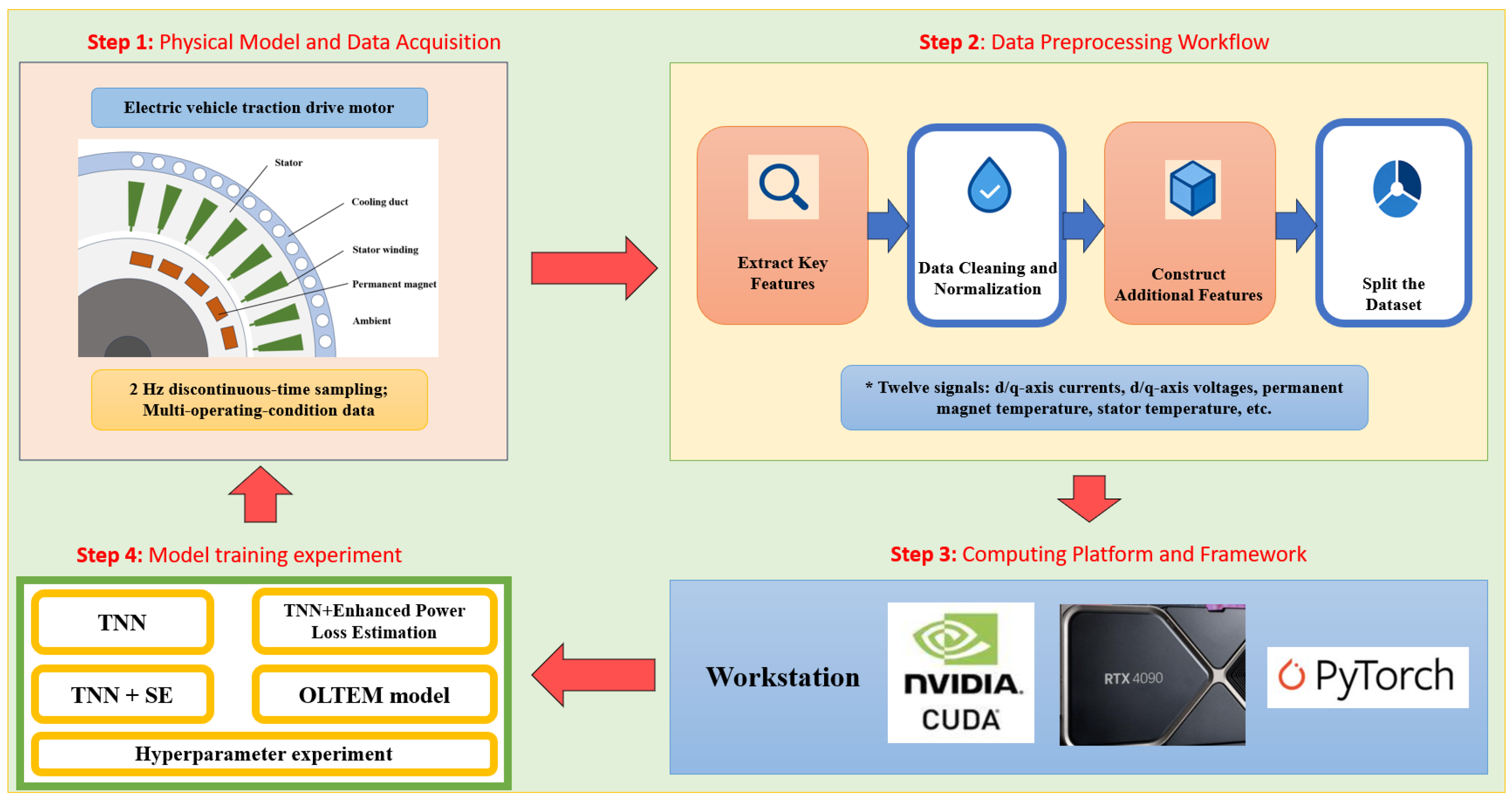
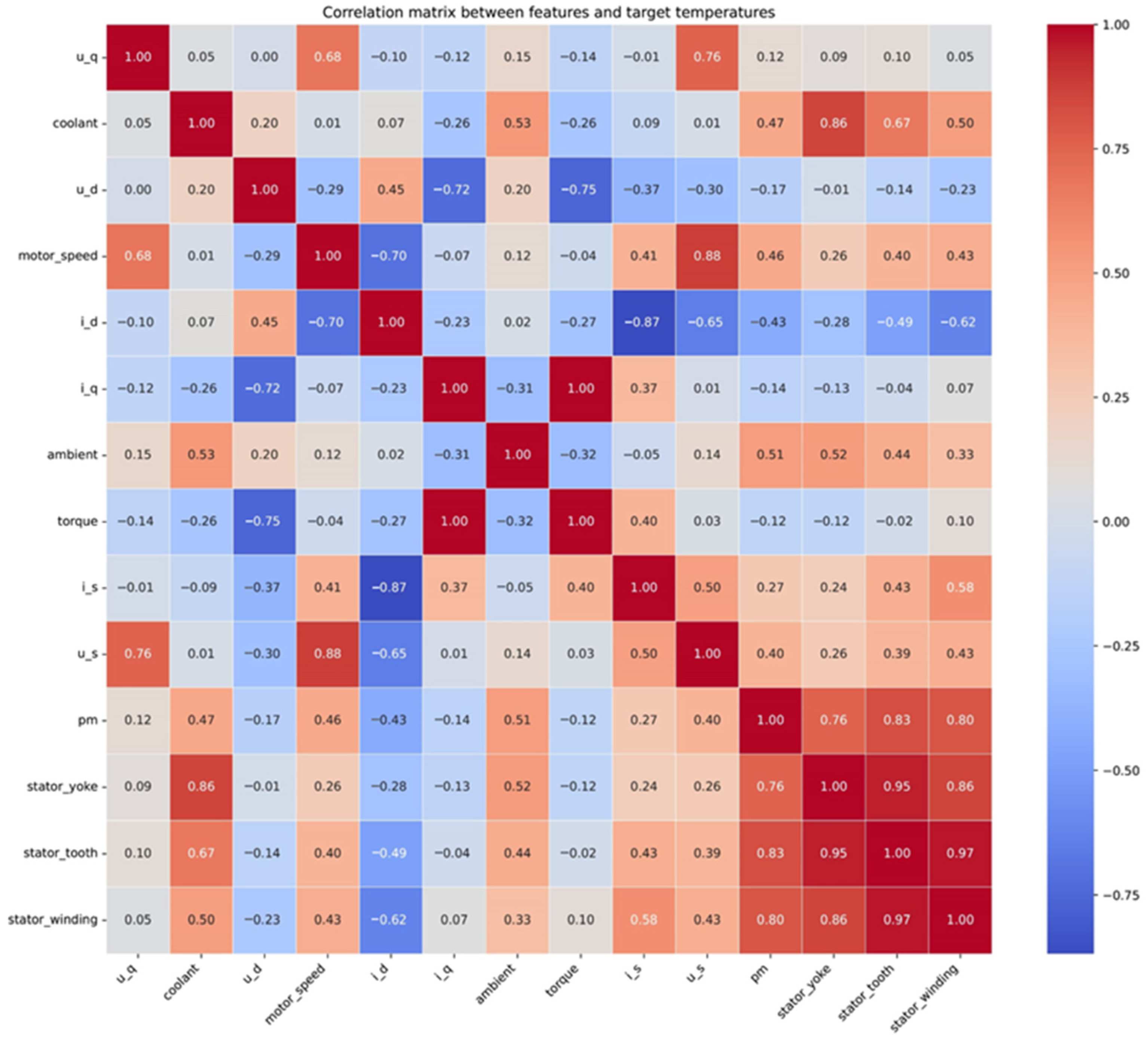
- Data Preprocessing: Initially, the raw data from the publicly available “Electric Motor Temperature” dataset on the Kaggle platform is cleaned, outliers are removed, and normalization is performed. To effectively capture the trends in motor operating conditions, two additional features are engineered from time-domain signals during the feature engineering phase: the current vector magnitude () and voltage vector magnitude () constructed from current and voltage signals, respectively. The dataset is then split into training and validation sets using profile id as the splitting criterion, with a ratio of 8:2. Additionally, a generalization set comprising three profile ids is retained within the overall dataset to ultimately assess the model’s ability to generalize.
- (b)
- Model Structure Setup: The model represents the temperature of each motor component as a node by introducing learnable inverse heat capacity parameters and a thermal conductance network, which simulate the system’s thermal dynamics through thermodynamic equations. The power loss module uses a deep network, physical constraints, and a dynamic load adjustment factor to handle complex conditions. Additionally, the SE module further highlights the significance of different input channels by assigning weights adaptively to each feature channel.
4. Experiments
4.1. Dataset
4.2. Evaluation Metrics and Baseline
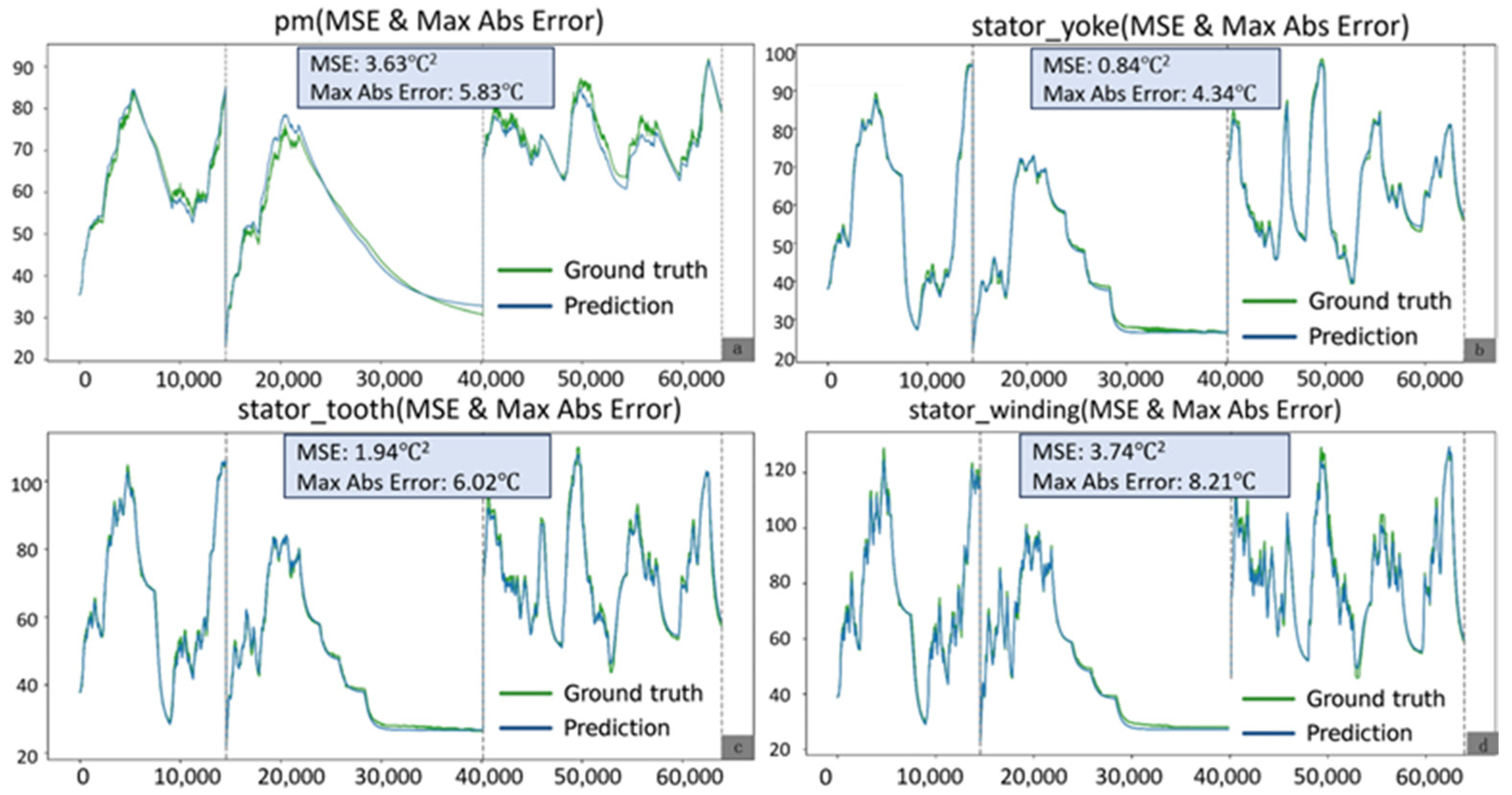
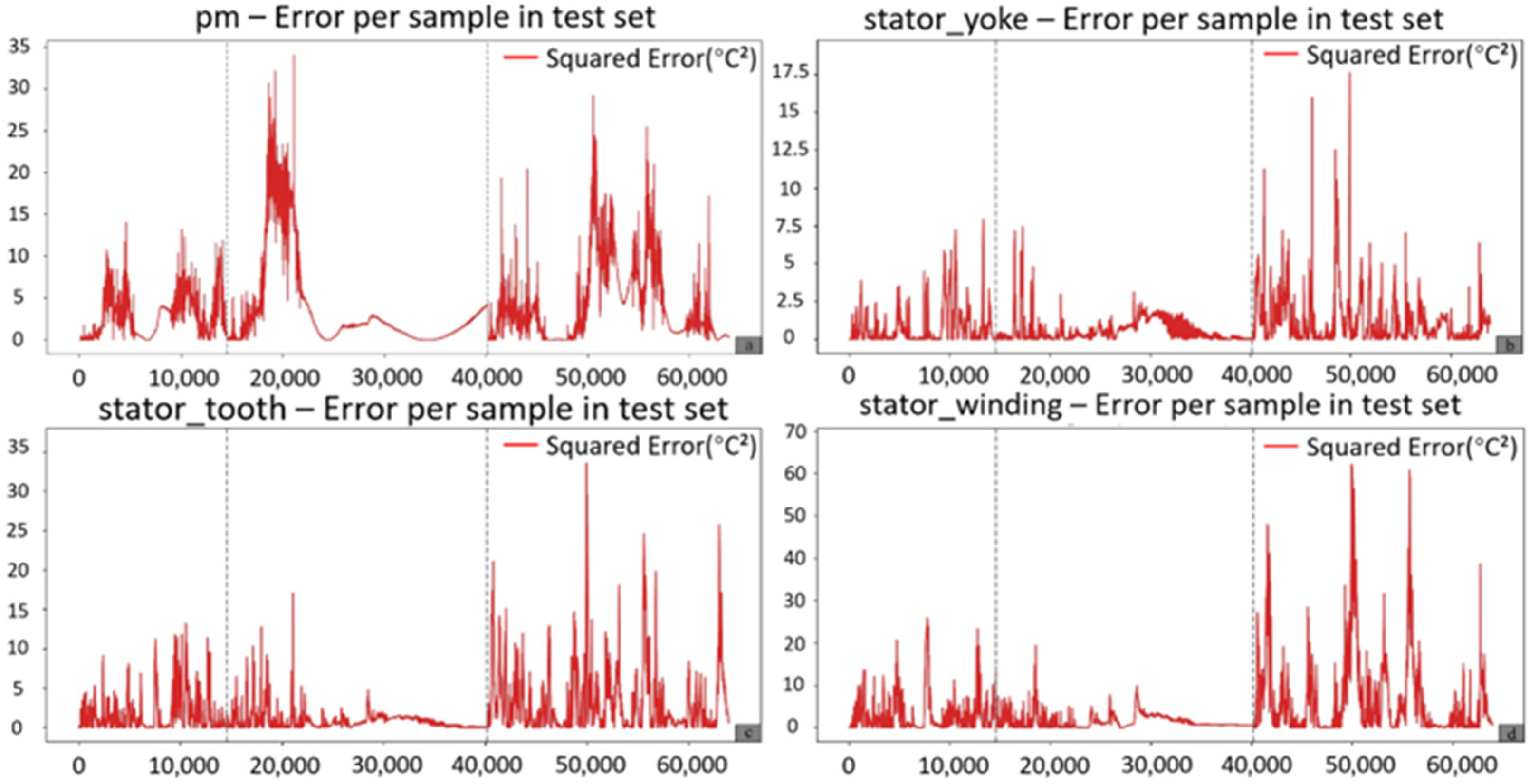
4.3. Experimental Evaluation and Comparative Analysis
5. Conclusions and Future Work
Author Contributions
Funding
Institutional Review Board Statement
Informed Consent Statement
Data Availability Statement
Acknowledgments
Conflicts of Interest
Abbreviations
| Specific heat capacity, J. kg−1·K−1 | |
| t | Time, s |
| p | Power loss per unit volume, W·m−3 |
| Heat capacity of the i-th node, dependent on ζ(t), J·K−1 | |
| Power loss of the i-th node, dependent on ζ(t), w | |
| Thermal resistance between nodes i and j, dependent on ζ(t), K·W−1 | |
| Normalized temperature estimate of the i-th node at time step k | |
| Hidden layer output of the l-th layer at time | |
| Hidden state weight matrix of the l-th layer (l ≥ 0) | |
| Input vector at time step k, including temperature and observations | |
| Flag for dedicated branch in π | |
| Initial learning rate | |
| Greek symbols | |
| Density, kg·m−3 | |
| Temperature, K−1 | |
| Thermal conductivity, W·m−1·K−1 | |
| Power loss of the i-th component at time step k, estimated by neural network, w−1 | |
| Thermal conductivity between nodes i and j at time step k, estimated by neural network, W·K−1 | |
| Inverse heat capacity of the i-th node at time step k, estimated by neural network, J−1·K−1 | |
| Subscripts | |
| p | Nanoparticle |
| i | Index of a node or component (e.g., the i-th node) |
| j | Index of a node or component (e.g., the j-th node) |
| k | Time step index or external node index |
| l | Neural network layer index |
| m | Number of auxiliary temperature nodes |
| n | Number of target temperature nodes |
| h | Related to hidden layers (e.g., ) |
| r | Related to recurrent connections (e.g., ) |
| s | Related to sampling or subsequences (e.g., , ) |
References
- Ahmed, S.; Siddiqi, M.R.; Ali, Q.; Yazdan, T.; Hussain, A.; Hur, J. Brushless Wound Rotor Synchronous Machine Topology Using Concentrated Winding for Dual Speed Applications. IEEE Access 2023, 11, 119560–119567. [Google Scholar] [CrossRef]
- Lin, H.; Wei, X.; Song, L.; Geng, H.; Li, L. Thermal Dissipation of High-Speed Permanent Magnet Synchronous Motor Considering Multi-field Coupling: Simulation Application and Experiment Realization. IEEE Access 2024, 12, 148625–148635. [Google Scholar] [CrossRef]
- König, P.; Sharma, D.; Konda, K.R.; Xie, T.; Höschler, K. Comprehensive review on cooling of permanent magnet synchronous motors and their qualitative assessment for aerospace applications. Energies 2023, 16, 7524. [Google Scholar] [CrossRef]
- Zhou, P.; Xu, Y.; Xin, F. Study of magneto-thermal problems in low-speed high-torque direct drive PMSM based on demagnetization detection and loss optimization of permanent magnets. IEEE Access 2023, 11, 92055–92069. [Google Scholar] [CrossRef]
- Fabian, M.; Hind, D.M.; Gerada, C.; Sun, T.; Grattan, K.T. Comprehensive monitoring of electrical machine parameters using an integrated fiber Bragg grating-based sensor system. J. Light. Technol. 2018, 36, 1046–1051. [Google Scholar] [CrossRef]
- Sharifi, T.; Eikani, A.; Mirsalim, M. Heat transfer study on a stator-permanent magnet electric motor: A hybrid estimation model for real-time temperature monitoring and predictive maintenance. Case Stud. Therm. Eng. 2024, 63, 105286. [Google Scholar] [CrossRef]
- Nasir, B.A. Sensor-less monitoring of induction motor temperature with an online estimation of stator and rotor resistances taking the effect of machine parameters variation into account. Int. J. Eng. Trends Technol. 2022, 70, 54–62. [Google Scholar] [CrossRef]
- Hasanzadeh, A.; Reed, D.M.; Hofmann, H.F. Rotor resistance estimation for induction machines using carrier signal injection with minimized torque ripple. IEEE Trans. Energy Convers. 2018, 34, 942–951. [Google Scholar] [CrossRef]
- Foti, S.; Testa, A.; De Caro, S.; Scelba, G.; Scarcella, G. Sensorless rotor and stator temperature estimation in induction motor drives. In Proceedings of the 2020 ELEKTRO, Taormina, Italy, 25–28 May 2020; IEEE: Piscataway, NJ, USA, 2020; pp. 1–6. [Google Scholar]
- Zhang, C.; Chen, L.; Wang, X.; Tang, R. Loss calculation and thermal analysis for high-speed permanent magnet synchronous machines. IEEE Access 2020, 8, 92627–92636. [Google Scholar] [CrossRef]
- Cao, L.; Fan, X.; Li, D.; Kong, W.; Qu, R.; Liu, Z. Improved LPTN-based online temperature prediction of permanent magnet machines by global parameter identification. IEEE Trans. Ind. Electron. 2022, 70, 8830–8841. [Google Scholar] [CrossRef]
- Huang, K.; Ding, B.; Lai, C.; Feng, G. Flux linkage tracking-based permanent magnet temperature hybrid modeling and estimation for PMSMs with data-driven-based core loss compensation. IEEE Trans. Power Electron. 2023, 39, 1410–1421. [Google Scholar] [CrossRef]
- Kirchgässner, W.; Wallscheid, O.; Böcker, J. Deep residual convolutional and recurrent neural networks for temperature estimation in permanent magnet synchronous motors. In Proceedings of the 2019 IEEE International Electric Machines & Drives Conference (IEMDC), San Diego, CA, USA, 12–15 May 2019; IEEE: Piscataway, NJ, USA, 2019; pp. 1439–1446. [Google Scholar]
- Kirchgässner, W.; Wallscheid, O.; Böcker, J. Estimating electric motor temperatures with deep residual machine learning. IEEE Trans. Power Electron. 2020, 36, 7480–7488. [Google Scholar] [CrossRef]
- Jing, H.; Chen, Z.; Wang, X.; Wang, X.; Ge, L.; Fang, G.; Xiao, D. Gradient boosting decision tree for rotor temperature estimation in permanent magnet synchronous motors. IEEE Trans. Power Electron. 2023, 38, 10617–10622. [Google Scholar] [CrossRef]
- MGarouani; Mothe, J.; Barhrhouj, A.; Aligon, J. Investigating the Duality of Interpretability and Explainability in Machine Learning. In Proceedings of the 2024 IEEE 36th International Conference on Tools with Artificial Intelligence (ICTAI), Herndon, VA, USA, 28–30 October 2024; pp. 861–867. [Google Scholar] [CrossRef]
- Kirchgässner, W.; Wallscheid, O.; Böcker, J. Thermal neural networks: Lumped-parameter thermal modeling with state-space machine learning. Eng. Appl. Artif. Intell. 2023, 117, 105537. [Google Scholar] [CrossRef]
- Hao, Z.; Liu, S.; Zhang, Y.; Ying, C.; Feng, Y.; Su, H.; Zhu, J. Physics-informed machine learning: A survey on problems, methods and applications. arXiv 2022, arXiv:2211.08064. [Google Scholar]
- Li, Y.; Xie, S.; Wang, J.; Zhang, J.; Yan, H. Sparse sample train axle bearing fault diagnosis: A semi-supervised model based on prior knowledge embedding. IEEE Trans. Instrum. Meas. 2023, 72, 1–11. [Google Scholar] [CrossRef]
- Zhang, T.; Chen, J.; He, S.; Zhou, Z. Prior knowledge-augmented self-supervised feature learning for few-shot intelligent fault diagnosis of machines. IEEE Trans. Ind. Electron. 2022, 69, 10573–10584. [Google Scholar] [CrossRef]
- Tang, P.; Zhao, Z.; Li, H. Transient Temperature Field Prediction of PMSM Based on Electromagnetic-Heat-Flow Multi-Physics Coupling and Data-Driven Fusion Modeling. SAE Int. J. Adv. Curr. Pract. Mobil. 2023, 6, 2379–2389. [Google Scholar]
- Liu, L.; Yin, W.; Guo, Y. Hybrid mechanism-data-driven iron loss modelling for permanent magnet synchronous motors considering multiphysics coupling effects. IET Electr. Power Appl. 2024, 18, 1833–1843. [Google Scholar] [CrossRef]
- Raouf, I.; Kumar, P.; Kim, H.S. Deep learning-based fault diagnosis of servo motor bearing using the attention-guided feature aggregation network. Expert Syst. Appl. 2024, 258, 125137. [Google Scholar] [CrossRef]
- Vo, T.T.; Liu, M.K.; Tran, M.Q. Harnessing attention mechanisms in a comprehensive deep learning approach for induction motor fault diagnosis using raw electrical signals. Eng. Appl. Artif. Intell. 2024, 129, 107643. [Google Scholar] [CrossRef]
- Gedlu, E.G.; Wallscheid, O.; Böcker, J. Permanent magnet synchronous machine temperature estimation using low-order lumped-parameter thermal network with extended iron loss model. In Proceedings of the 10th International Conference on Power Electronics, Machines and Drives (PEMD 2020), London, UK, 15–17 December 2020; IET: London, UK, 2020; Volume 2020, pp. 937–942. [Google Scholar]
- Rong, C.; Zhang, Q.; Zhu, Z.; Li, H.; Huang, Z.; Zhang, D.; Wu, T. Iron Loss Calculation and Thermal Analysis of High-Speed Permanent Magnet Synchronous Motors Under Various Load Conditions. In Proceedings of the 2023 26th International Conference on Electrical Machines and Systems (ICEMS), Zuhai, China, 5–8 November 2023; IEEE: Piscataway, NJ, USA, 2023; pp. 2158–2163. [Google Scholar]
- Ba, X.; Gong, Z.; Guo, Y.; Zhang, C.; Zhu, J. Development of equivalent circuit models of permanent magnet synchronous motors considering core loss. Energies 2022, 15, 1995. [Google Scholar] [CrossRef]
- Tüysüz, A.; Schaubhut, A.; Zwyssig, C.; Kolar, J.W. Model-based loss minimization in high-speed motors. In Proceedings of the 2013 International Electric Machines & Drives Conference, Chicago, IL, USA, 12–15 May 2013; IEEE: Piscataway, NJ, USA, 2013; pp. 332–339. [Google Scholar]
- Liu, Z.; Kong, W.; Fan, X.; Li, Z.; Peng, K.; Qu, R. Hybrid Thermal Modeling with LPTN-Informed Neural Network for Multi-Node Temperature Estimation in PMSM. IEEE Trans. Power Electron. 2024, 39, 10897–10909. [Google Scholar] [CrossRef]
- Wallscheid, O.; Böcker, J. Global identification of a low-order lumped-parameter thermal network for permanent magnet synchronous motors. IEEE Trans. Energy Convers 2015, 31, 354–365. [Google Scholar] [CrossRef]
- Jie, H.; Li, S.; Gang, S. Squeeze-and-Excitation Networks. In Proceedings of the IEEE Conference on Computer Vision and Pattern Recognition, Salt Lake City, UT, USA, 18–22 June 2018; p. 5. [Google Scholar]
- Liang, J.; Liang, K.; Shao, Z.; Niu, Y.; Song, X.; Sun, P.; Feng, J. Research on Temperature-Rise Characteristics of Motor Based on Simplified Lumped-Parameter Thermal Network Model. Energies 2024, 17, 4717. [Google Scholar] [CrossRef]
- Fan, Y.; Feng, W.; Ren, Z.; Liu, B.; Wang, D. Lumped Parameter Thermal Network Modeling and Thermal Optimization Design of an Aerial Camera. Sensors 2024, 24, 3982. [Google Scholar] [CrossRef] [PubMed]


| Hyperparameter | Optimum |
|---|---|
| Minimum validation MSE(C2) | 1.39 |
| Learning rate | 0.001937 |
| Optimizer | RMSprop |
| ploss_hidden_dim | 112 |
| Leaky ReLU slope | 0.2104 |
| Parameter Name | Description | Unit |
|---|---|---|
| u_q | Voltage q-axis component | V |
| u_d | Voltage d-axis component | V |
| coolant | Coolant temperature | °C |
| stator_yoke | Stator yoke temperature | °C |
| stator_tooth | Stator tooth temperature | °C |
| stator_winding | Stator winding temperature | °C |
| motor_speed | Motor speed | rpm |
| i_d | Current d-axis component | A |
| i_q | Current q-axis component | A |
| pm | Permanent magnet temperature | °C |
| ambient | Ambient temperature | °C |
| torque | Torque generated by the current | N·m |
| pm | stator_yoke | stator_tooth | stator_winding | |||||
|---|---|---|---|---|---|---|---|---|
(°C2) | (°C) | (°C2) | (°C) | (°C2) | (°C) | (°C2) | (°C) | |
| TNN | 5.16 | 6.6 | 2.32 | 6.1 | 3.38 | 6.9 | 6.38 | 9.8 |
| CNN-RNN | 4.36 | 5.3 | 1.51 | 6.2 | 2.15 | 5.2 | 5.22 | 9.0 |
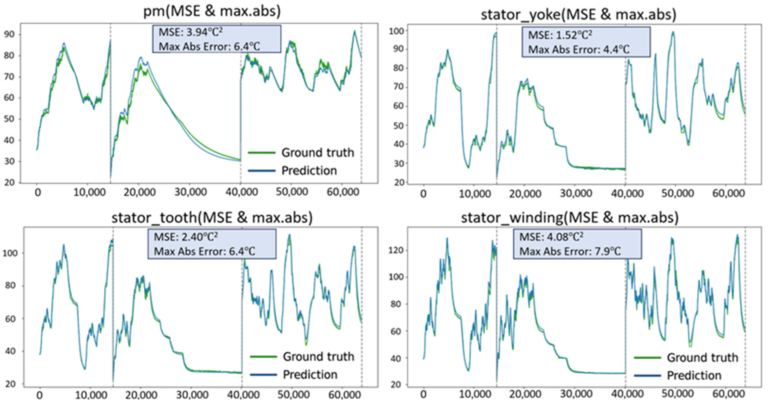
| OLTEM–SC-SE | 3.94 | 6.4 | 1.52 | 4.4 | 2.4 | 6.4 | 4.08 | 7.9 |
| OLTEM–Enhanced Power Loss Estimation Module | 4.58 | 6.3 | 1.99 | 5.1 | 3.04 | 6.2 | 4.37 | 8.6 |
| OLTEM | 3.77 | 5.7 | 0.91 | 5.4 | 2.11 | 7.3 | 3.31 | 9.1 |
Disclaimer/Publisher’s Note: The statements, opinions and data contained in all publications are solely those of the individual author(s) and contributor(s) and not of MDPI and/or the editor(s). MDPI and/or the editor(s) disclaim responsibility for any injury to people or property resulting from any ideas, methods, instructions or products referred to in the content. |
© 2025 by the authors. Licensee MDPI, Basel, Switzerland. This article is an open access article distributed under the terms and conditions of the Creative Commons Attribution (CC BY) license (https://creativecommons.org/licenses/by/4.0/).
Share and Cite
Sheng, Y.; Liu, X.; Chen, Q.; Zhu, Z.; Huang, C.; Wang, Q. OLTEM: Lumped Thermal and Deep Neural Model for PMSM Temperature. AI 2025, 6, 173. https://doi.org/10.3390/ai6080173
Sheng Y, Liu X, Chen Q, Zhu Z, Huang C, Wang Q. OLTEM: Lumped Thermal and Deep Neural Model for PMSM Temperature. AI. 2025; 6(8):173. https://doi.org/10.3390/ai6080173
Chicago/Turabian StyleSheng, Yuzhong, Xin Liu, Qi Chen, Zhenghao Zhu, Chuangxin Huang, and Qiuliang Wang. 2025. "OLTEM: Lumped Thermal and Deep Neural Model for PMSM Temperature" AI 6, no. 8: 173. https://doi.org/10.3390/ai6080173
APA StyleSheng, Y., Liu, X., Chen, Q., Zhu, Z., Huang, C., & Wang, Q. (2025). OLTEM: Lumped Thermal and Deep Neural Model for PMSM Temperature. AI, 6(8), 173. https://doi.org/10.3390/ai6080173