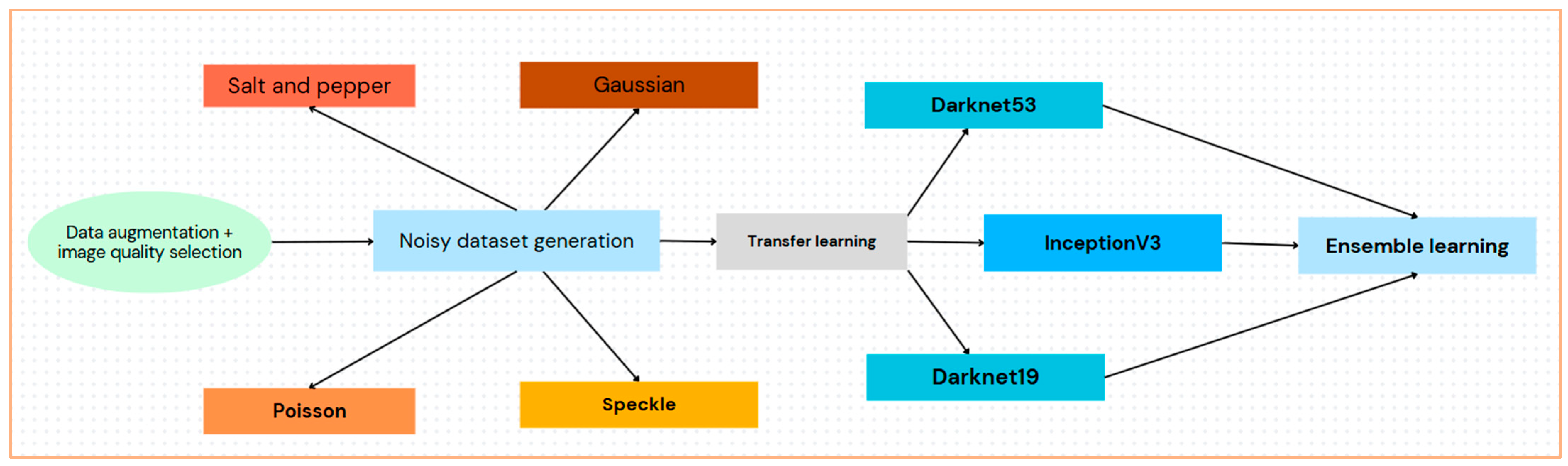
3. Materials and Methods
The methodology included quality selection, augmentation, noise modeling and generation, feature extraction via transfer learning, and classification by ensemble learning, as illustrated in
Figure 2.
Our proposed approach utilized an ensemble of pre-trained DNNs, overcoming the challenge of limited medical image data and noise existence challenges on medical images through augmentation and transfer learning.
Neural network performance is greatly impacted by image quality, and accuracy can be deteriorated by inconsistent training and testing data [
41,
42]. Data augmentation is a popular method for lowering overfitting in DNN training [
43,
44]. A variety of augmentation techniques are used to create various images, such as ultrasound images, including rotation, projective transformation, warping, and cropping. An upgraded image data store was utilized for automatic scaling to preserve homogeneity. Random vertical flipping, translation up to 30 pixels, and 10% scaling in both directions were additional modifications. By avoiding overfitting and dependence on image characteristics, these augmentations aid in enhancing model generalization.
For training and testing, we used a dataset that consists of a total of 4413 ultrasound images, classified into ‘normal’ (1821 images) and ‘stone’ (2592 images), gathered from a dataset that contains 5431 open-source normal kidney and kidneys with stones images plus a pre-trained kidney-stone-ultrasound model and API [
45] while maintaining privacy. Images were collected across multiple clinical sites, including mid-range portable devices (Mindray which are produced by Shenzhen Mindray Bio-Medical Electronics Co., Ltd., headquartered in Shenzhen, China, GE Logiq which are manufactured by GE HealthCare, in Wauwatosa, Wisconsin, United States, and Philips which are manufactured by Philips Healthcare, in Bothell, Washington, United States) and console systems. Gain was adjusted on a per-scan basis by operators to ensure optimal contrast between kidney parenchyma and stones. Displayed gain variations are visible in image brightness. Depth settings ranged from approximately 8 cm to 16 cm, depending on patient size and kidney location. Scans included transverse, longitudinal, and oblique views, chosen to best visualize stone echogenicity and acoustic shadows. The selected 4413 images in this study were the clearly labelled images as either ‘normal’ or ‘stone’ out of the 5431 images. The dataset was partitioned as follows: 60% was used for training, 20% was used for testing, and the remaining 20% was used for validation.
Images undergo preprocessing to correct distortions and lighting issues before object detection. This included resizing, grayscale conversion, and pixel normalization to match model input sizes. For instance, ResNet requires a 240 × 240 input size.
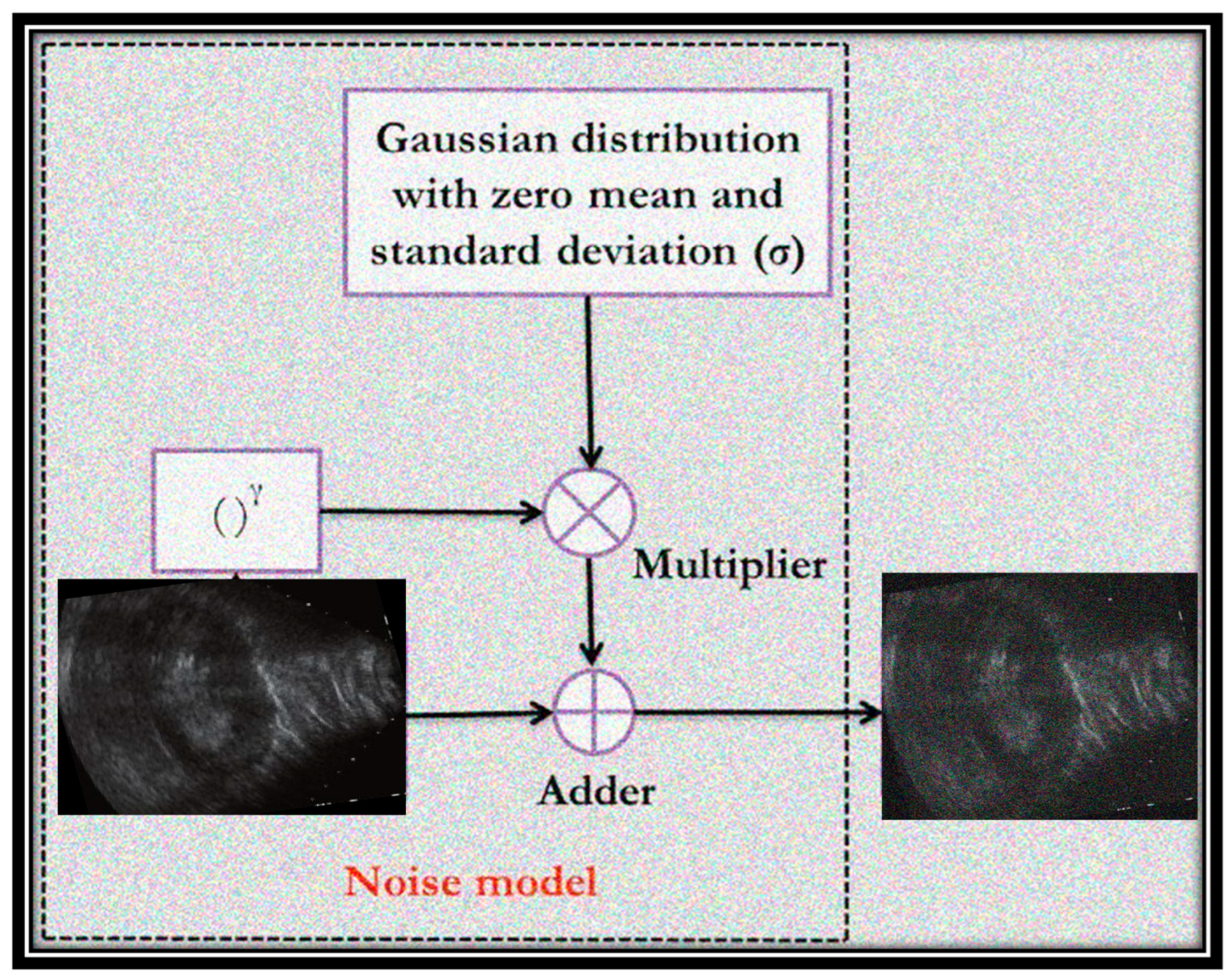
The images used in the dataset of this study were modified by adding different types of noise: speckle, salt and pepper, Poisson, and Gaussian.
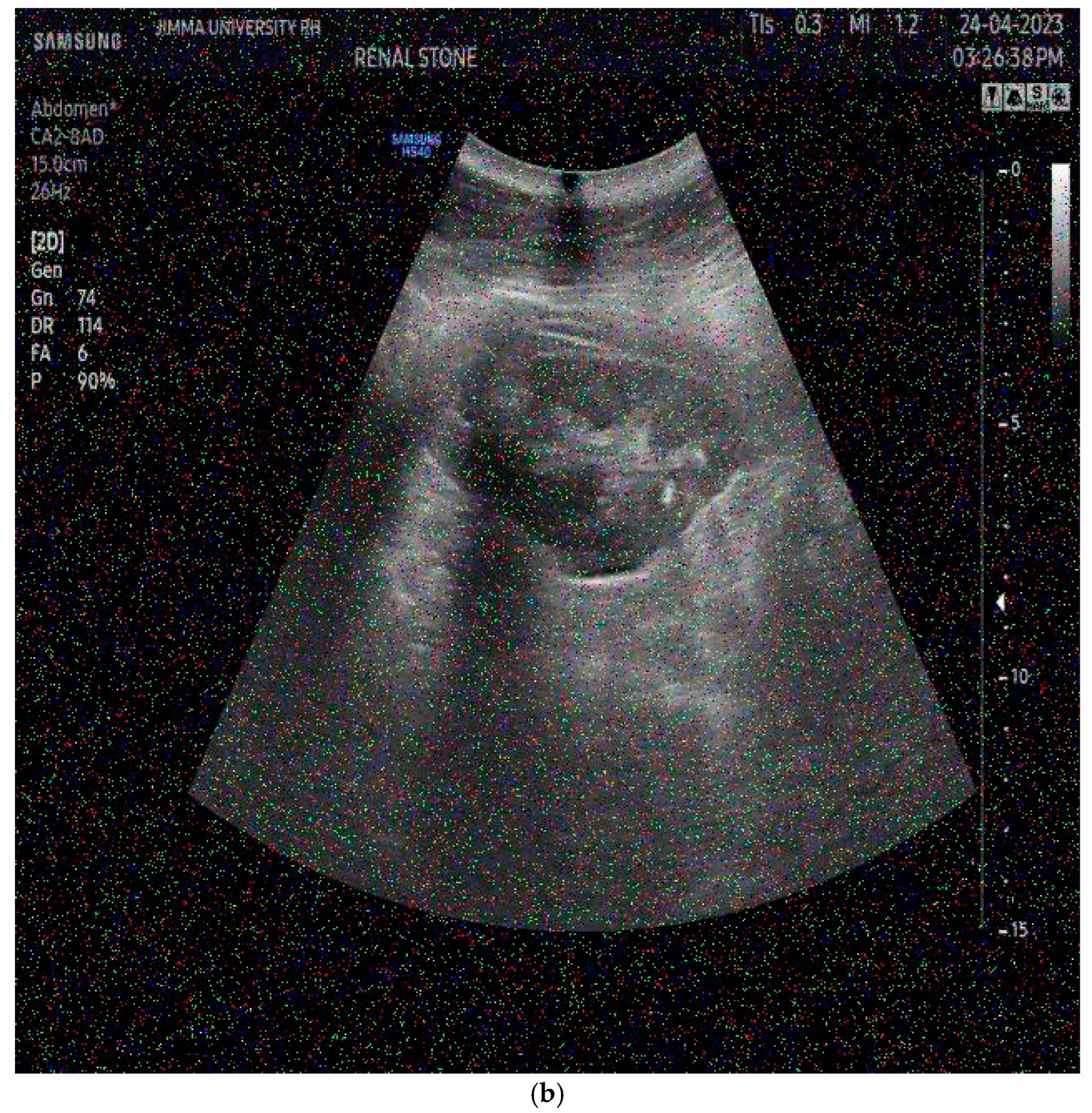
Figure 3 shows an example of a Gaussian distributed noise model with zero mean and a specific standard deviation that corrupts images with two example ultrasound images (before and after noise addition). The additional values of noisy pixels are added to the original image to create the noisy image. It can be noted that the randomly distributed pixels have random RGB values and colors.
To ensure reliability, the noise was added randomly, where each image was associated with one random noise type. Moreover, each noise was added with a random variance value to demonstrate high reliability and performance. Noise was added to both training and testing images.
Speckle noise is formed as follows:
where
fn (
x,
y) is the image after adding the speckle noise,
f (
x,
y) is the image without added noise, and
η(
x,
y) is a zero-mean and zero-variance Gaussian distribution. The term
γ refers to the multiplicative noise model when its value is 1. The variance or density values of speckle noise, as well as other noise types, were chosen randomly for each image, ranging from 0.01 to 0.1.
Salt and pepper noise replaces some pixels in the image with either 0 or 255. It can be expressed as follows:
where
Ns value is the maximum pixel value (salt noise) and
Np value is the minimum pixel value (pepper noise). The expression
x(
i,
j) is the pixel value after corruption with the added noise.
γ refers to the value of noisy density.
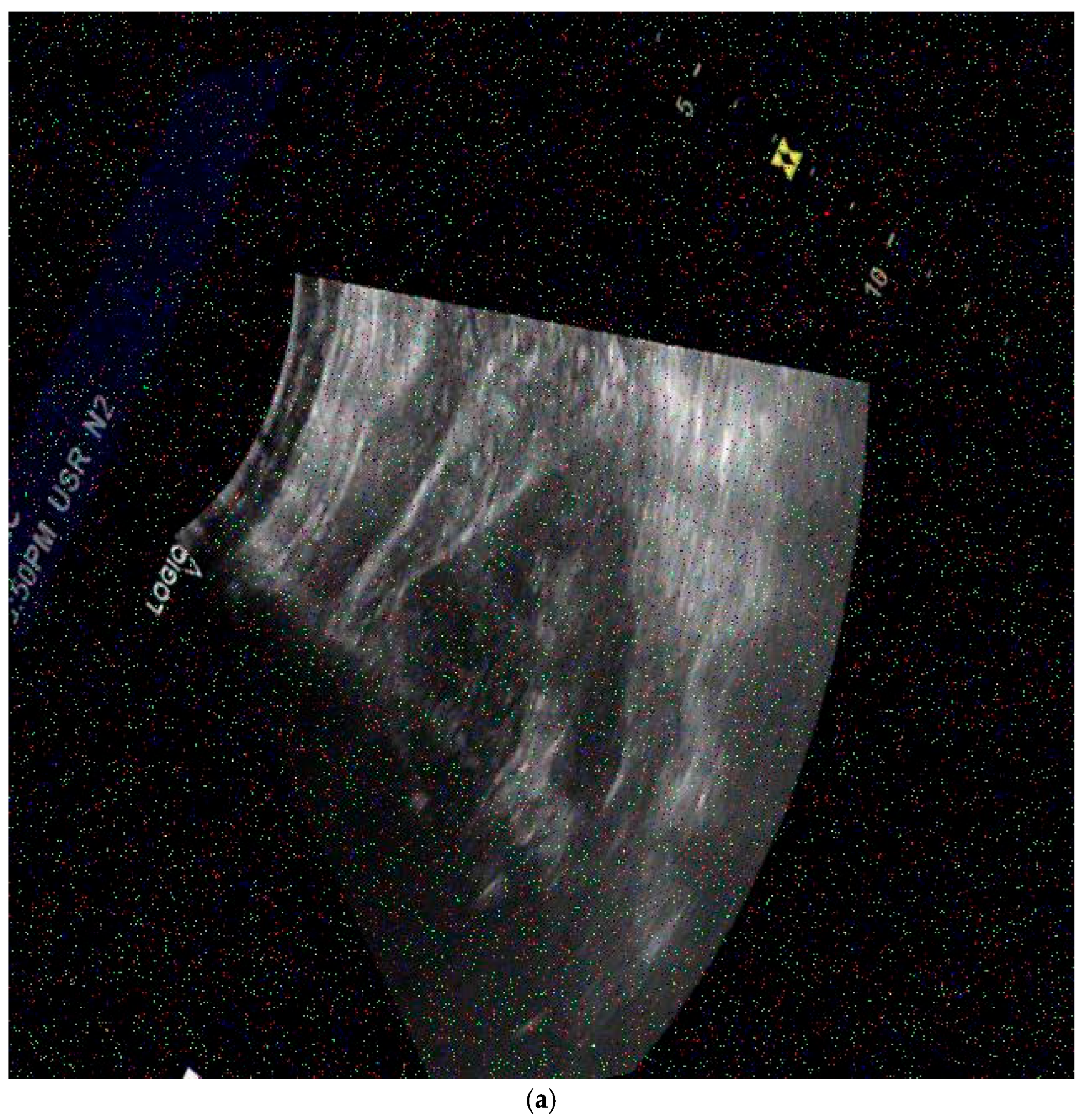
Figure 4 shows examples of noisy generated ultrasound images that were used for training or testing. The noise type is random, as well as the variance/density values.
The peak signal to noise ratio (PSNR) is a quality measurement calculated value that is used to evaluate images in the area of image processing. PSNR can be obtained by the logarithm of the mean squared error (MSE) value of an image. Since grayscale images are 2D, the value of MSE is found concerning the
M ×
N dimensions of the image, calculated as follows:
where
M,
N, and
O refer to channels;
I() refers to the pixel value at
x,
y; and
I′ is the output image.
PSNR can be calculated as follows:
where
m is the largest scale value.
In our experiments, we added the noise to simulate real-world degradation in ultrasound images. For each image, one of four noise types, Gaussian, Poisson, salt and pepper, or speckle, was randomly applied. The selection was performed by a uniform discrete distribution, which ensures equal probability (25%) for each noise type. For Gaussian, salt and pepper, and speckle noise, the noise level (variance or density) was drawn uniformly at random from the interval [0.01,0.1]. Poisson noise does not take a variance parameter and was applied in its default configuration. This random noise generation procedure was applied independently to each image in both the training and testing sets, ensuring a uniform and unbiased distribution of noise types and intensities across the dataset. This approach provides sufficient variability while also ensuring that the methodology is reproducible, as the ranges used are explicitly defined.
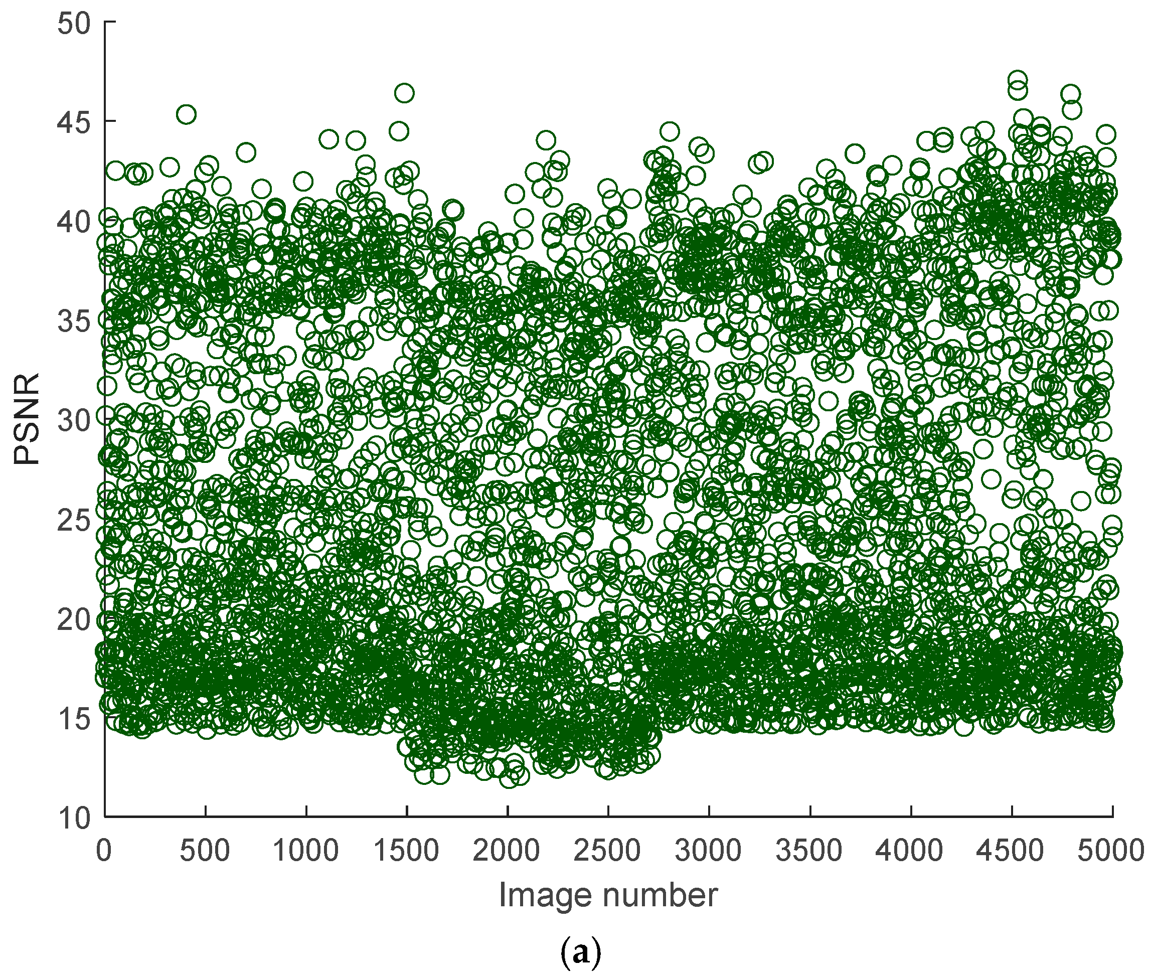
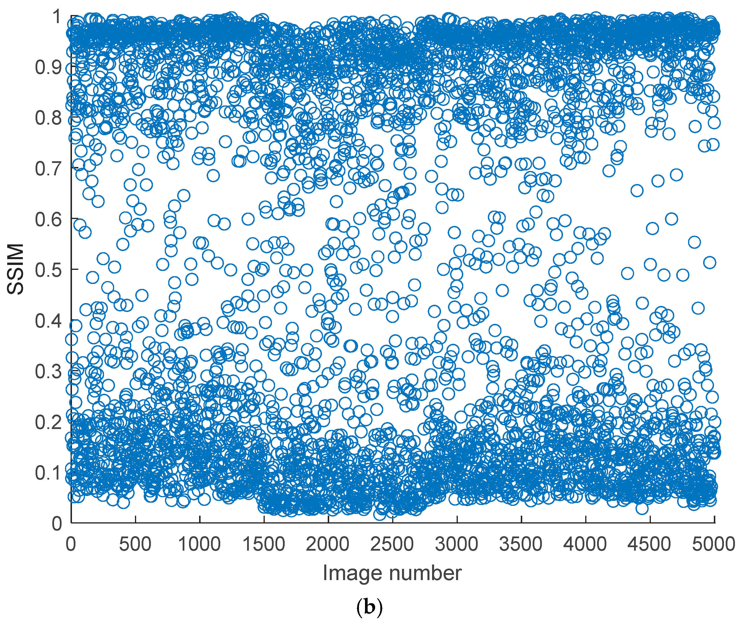
Figure 5 shows the measured PSNR and Structural Similarity Index (SSIM) values of some noisy kidney ultrasound images concerning the original corresponding ultrasound images. Based on the figure, the trends of PSNR and SSIM reveal significant variability in quality and structural integrity. PSNR values range from 10 dB to 50 dB, indicating a broad spectrum of image fidelity. High PSNR values (>40 dB) suggest near-lossless quality, likely from small noise intensity and distribution, while lower values (20–30 dB) are typical for lossy compression or mild noise. An extremely low PSNR (<20 dB) points to severe distortions, such as synthetic corruptions. PSNR’s limitations are evident, it fails to penalize blur or perceptual distortions adequately and is sensitive to global intensity shifts, which may not align with human perception. This makes PSNR more suitable for quantifying noise reduction in technical applications rather than assessing visual quality.
On the other hand, SSIM values are consistently low, ranging from 0.1 to 0.7, with most scores below 0.5. This indicates moderate to severe structural degradation across the dataset, with no images approaching the ideal score of 1. The stability of SSIM trends, compared to PSNR, suggests systemic structural distortions, possibly from a preprocessing step or inherent dataset issues. SSIM’s sensitivity to luminance, contrast, and structure makes it better correlate with human judgment, particularly for localized distortions like edge artifacts. However, the absence of high SSIM outliers implies that the dataset lacks pristine images. The divergence between PSNR and SSIM is notable; some images with a moderate PSNR (30–40 dB) exhibit a low SSIM (~0.3), highlighting PSNR’s inability to capture structural degradation, such as blur or texture loss. Conversely, noisy but structurally intact images may have a low PSNR but a moderate SSIM.
The joint analysis of PSNR and SSIM reveals critical insights into the dataset’s composition and potential biases. For instance, a high PSNR with a low SSIM often occurs in blurry denoised images, where noise reduction sacrifices texture details. A low PSNR with a moderate SSIM might reflect noisy but structurally preserved images, such as those with film grain.
Transfer learning can be utilized effectively for classification and detection. To learn general characteristics, a network is trained on a sizable collection of tagged natural images via transfer learning, and then those features are applied to classify other datasets. In our approach, DNN models, trained with images from a source domain, are used to classify kidney ultrasound images into either normal or stones for multiple cases. Features extracted during training are passed to a SoftMax classifier. We used three pre-trained DNNs, Darknet19, Darknet53, and Inceptionv3, to classify kidney ultrasound images into either two categories (normal and stones) or four categories: the first case is for the original dataset, the second case is when noise was added to all images (normal and stones), and the third case is the original dataset (normal and stones), besides the noisy dataset (noisy normal and noisy stones).
The pre-trained models help extract features from the kidney images, which are then used for classification. Since the method uses an ensemble of these models, the predictions from all three networks are combined to produce the final result.
The ensemble method improves classification by combining predictions from multiple models [
46,
47], reducing variance [
48] and bias [
49]. This approach ensembles three pre-trained DNNs for accurate kidney ultrasound image classification. Majority voting is used, where each model votes on a test instance, and the final prediction is based on the majority vote, enhancing overall model performance.
Our goal was to create a lightweight, computationally efficient ensemble. Inceptionv3 and Darknet53 have a deep architecture with 48 and 53 layers, respectively, while Darknet19 has fewer layers, requiring less computational power.
Table 1 compares three convolutional neural network architectures—InceptionV3, Darknet19, and Darknet53—across four critical hyperparameters directly influencing model performance and practical deployment. These parameters include network depth, parameter memory footprint, total trainable parameters, and required input image dimensions. Each architecture presents unique trade-offs between computational complexity, feature extraction capability, and hardware requirements, making them suitable for clinical scenarios.
The comparison reveals important technical trade-offs that inform clinical implementation decisions. Darknet19 emerges as the optimal choice for edge devices and point-of-care applications due to its compact size and efficient operation. InceptionV3 provides a middle ground, offering enhanced feature detection capabilities while remaining within reasonable computational limits. Darknet53 serves as a premium solution for high-accuracy diagnostic workstations where hardware resources are abundant. The ensemble approach combining all three networks likely capitalizes on their complementary strengths, using Darknet19 for initial screening, InceptionV3 for intermediate processing, and Darknet53 for the final confirmation of challenging cases.
These architectural differences also highlight important considerations for clinical workflow integration. The memory requirements directly impact deployment feasibility, with Darknet53’s 159 MB footprint potentially limiting its use in mobile applications. Input resolution requirements affect preprocessing pipelines, where InceptionV3’s 299 × 299 images may require a more substantial transformation of source images than the 256 × 256 standards of the Darknet variants. The parameter counts correlate with model expressiveness, explaining why Darknet53 achieves a high accuracy despite its greater resource consumption.
The deep learning models used in medical image classification, including those in this study, are primarily pre-trained on large-scale, natural image datasets such as ImageNet (ILSVRC). This dataset, which includes over 1.2 million images from 1000 object categories, serves as the source domain for transfer learning. While ImageNet images are from non-medical, natural scenes, the models learn generalizable low- and mid-level visual features that are useful for downstream tasks in medical imaging, the target domain.
InceptionV3, GoogLeNet, and EfficientNetB0 were pre-trained on ImageNet and adapted for medical use by replacing their final classification layers with domain-specific output heads. These models benefit from their architectural ability to capture multi-scale spatial features, which are particularly useful when identifying structures like kidney stones or tissue textures in ultrasound images.
Darknet19 and Darknet53 were also pre-trained on ImageNet. These models are particularly adept at real-time object localization and detection, which translates well into identifying distinct echogenic regions, such as renal stones in ultrasound scans. In medical adaptation, their classification layers are modified and fine-tuned on annotated medical data.
AlexNet and ResNet variants (ResNet18, ResNet50, and ResNet101) were also trained on ImageNet. The ResNet family, known for its residual learning capabilities, helps in training deeper models without vanishing gradient issues. These models transfer well to ultrasound imaging tasks due to their ability to extract deep hierarchical features that capture both low-level texture and high-level anatomical patterns.
MobileNetV2 also originates from ImageNet training. Its depth-wise separable convolutions make it computationally efficient, allowing adaptation to medical scenarios where lightweight models are essential, especially in point-of-care or portable ultrasound systems.
Vision Transformers (ViTs) are pre-trained on large datasets like ImageNet-21k or JFT-300M. In the medical domain, they are fine-tuned to learn spatial and contextual dependencies, which can be beneficial for tasks requiring attention to specific anatomical regions, such as stone localization or tissue classification in grayscale images.
In adapting all these models to the medical domain, transfer learning plays a central role. It involves retaining the learned convolutional or transformer-based features from the source domain and fine-tuning the models on a target medical dataset. Additionally, domain adaptation techniques, such as image preprocessing, data augmentation (rotation, scaling, shifting), and regularization, are applied to bridge the domain gap between natural and medical images. This adaptation enhances performance, especially when working with relatively small annotated medical datasets compared to ImageNet-scale datasets.
4. Simulation Results and Discussion
In this section, the experimental settings are demonstrated, including the used dataset, the performance outcomes, and the comparisons with other related works.
The experiments were performed using the following specifications. A Core i7 Intel PC with 2.8 GHz and 4 TB SSD storage were used. The operating system of the PC was 64 bit with 16 GB of RAM. The computational tasks were performed using an NVIDIA 1050 GPU.
The dataset is publicly available [
45], containing 4413 images classified into ‘normal’ (1821 images) and ‘stone’ (2592 images). The dataset was gathered from a clinic while maintaining patient privacy. Some images were rotated, translated, or with varying viewpoints and projections. Moreover, the intensity and lighting of some images were low, representing significant challenges. The size of each image was 640 × 640.
An augmented image data store was used to resize the images. Additionally, augmentation methods were used, such as random flipping, random translation, and random scaling in both height and width, to help reduce overfitting by ensuring learning general patterns instead of memorizing details.
The training configuration utilizes a mini-batch size of 10. This choice balances between convergence speed and computational efficiency.
The initial learning rate was set to 0.0003 to ensure stable convergence and prevent the model from overshooting the optimal weights.
Training data were shuffled at every epoch to ensure that the model does not learn the order of the samples and generalizes better. All models in this study were trained and used with the same options and settings to ensure fairness in performance evaluations.
Training and testing were performed using five cases described as follows:
The original kidney images without added noise (normal kidney images and images with kidney stones), besides the dataset with added random Gaussian noise.
The dataset without added noise (normal kidney images and images with kidney stones), besides the dataset with added random speckle noise.
The dataset without added noise (normal kidney images and images with kidney stones), besides the dataset with added random Poisson noise.
The dataset without added noise (normal kidney images and images with kidney stones), besides the dataset with added random salt and pepper noise.
The dataset without added noise (normal kidney images and images with kidney stones), besides the dataset with added random noise using a random type from any of the four noise types (Gaussian, Poisson, speckle, or salt and pepper).
The evaluations were assessed using metrics such as precision, recall, accuracy, specificity, and F1 score. The F1 score is used when there is a trade-off between precision and recall, especially in scenarios where minimizing false positives or false negatives is critical. It represents the harmonic means of precision and recall, providing a balanced metric that accounts for both measures. The F1 score is useful in maintaining an equilibrium between these metrics to ensure a comprehensive evaluation of the model’s performance.
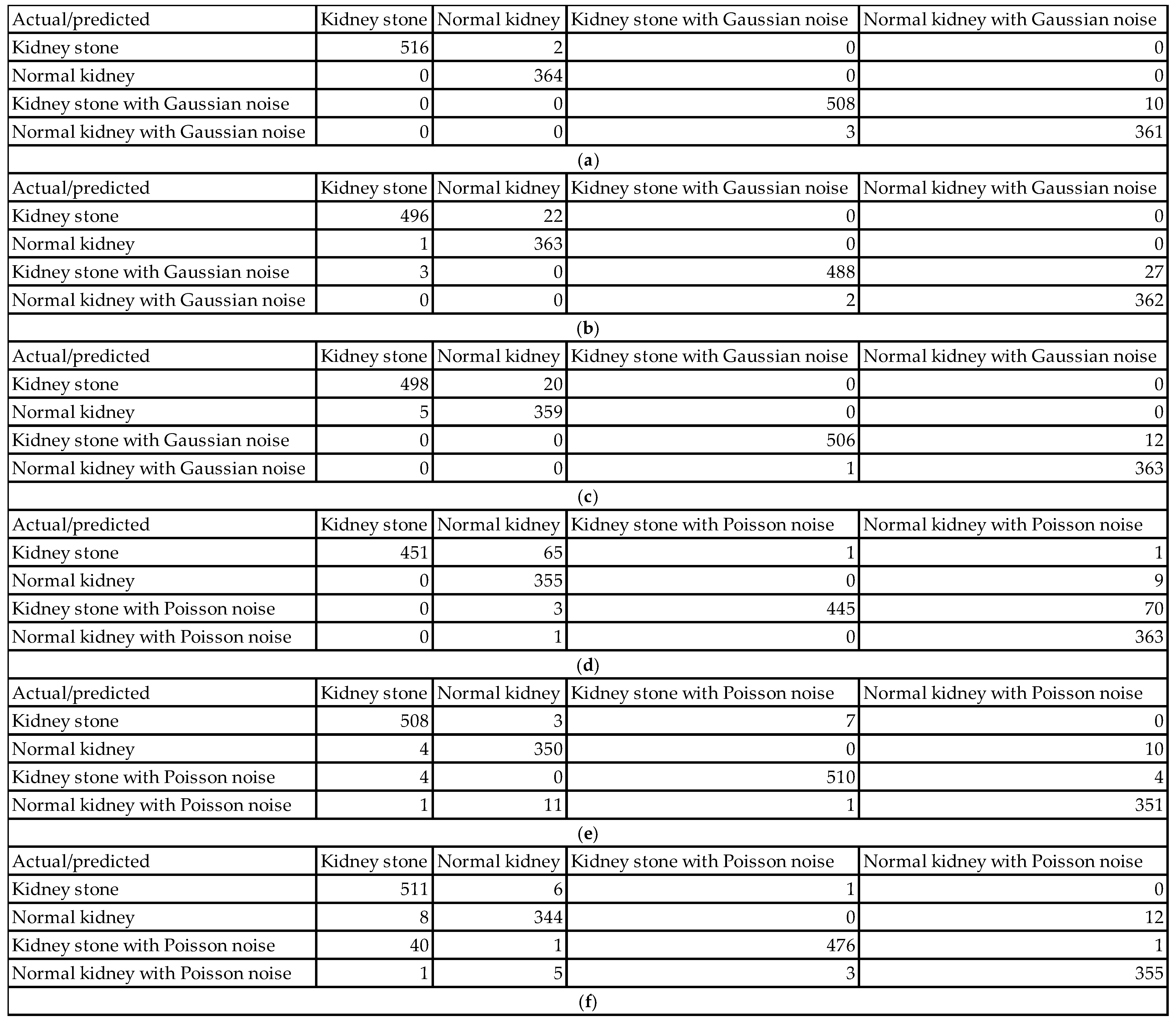
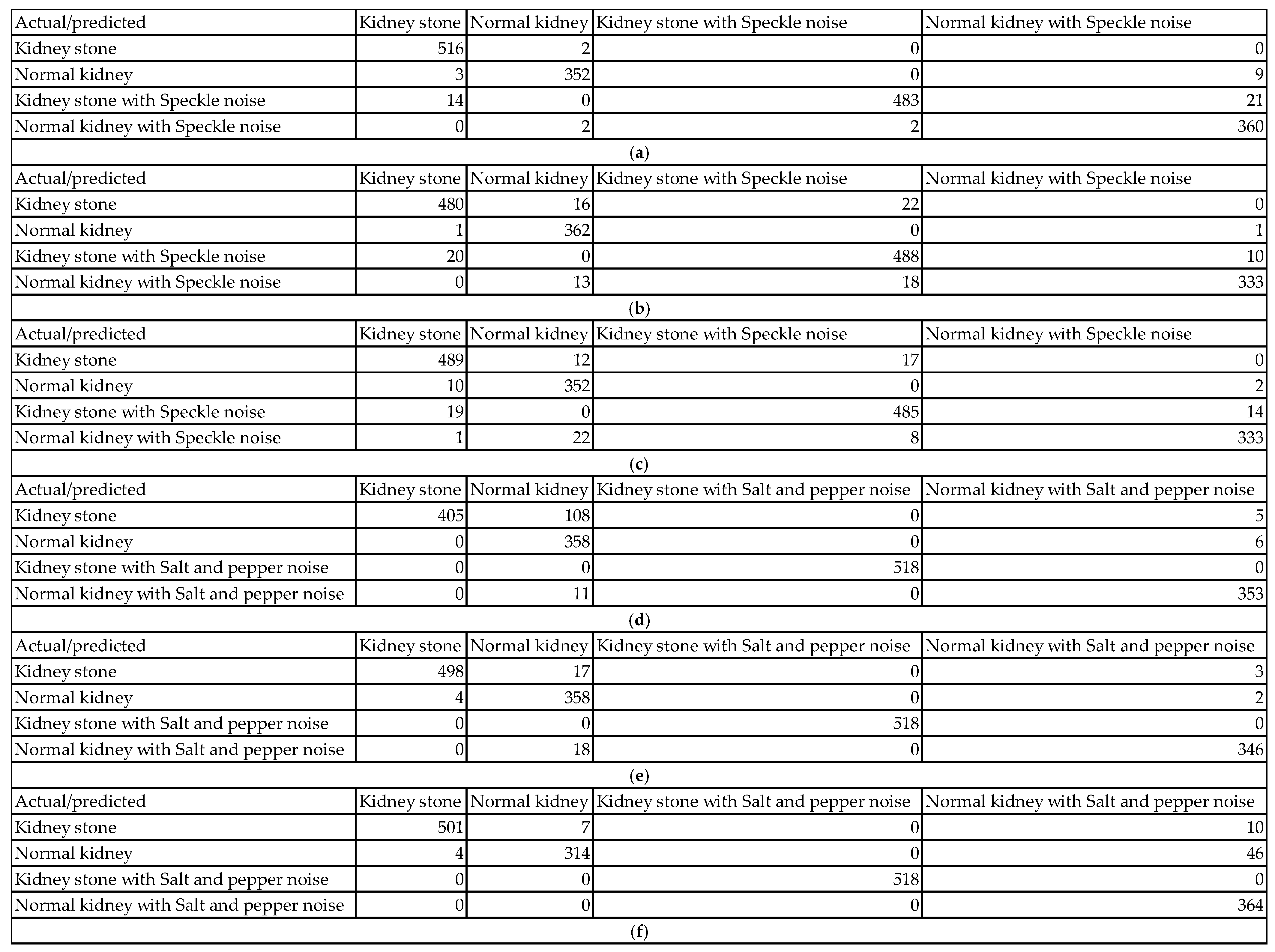
Figure 6 and
Figure 7 show examples of the obtained confusion matrices for the classification results of the dataset (using InceptionV3, Darknet19, and Darknet53), besides the dataset and added Gaussian or Speckle noises.
The classification performance evaluation in
Figure 6 using confusion matrices for InceptionV3, Darknet19, and Darknet53 models on a kidney ultrasound dataset, comprising both original and Gaussian-noise-augmented images, revealed clear distinctions in accuracy and robustness. Each confusion matrix summarizes the model’s predictions across four classes: kidney stone cases, normal kidney cases, and their counterparts with Gaussian noise. The results highlight how each model handles clean versus noisy inputs and its ability to differentiate between pathological and healthy conditions.
InceptionV3 achieved the highest performance among the three models. It classified 516 out of 518 kidney stone cases and all 364 normal kidney cases correctly. On noisy data, it accurately classified 508 of 518 kidney stone cases with Gaussian noise and 361 of 364 normal kidney cases with Gaussian noise. Misclassifications were minimal, with only 13 errors in total, most of which involved noisy data being incorrectly labeled within its noisy class. This reflects InceptionV3’s exceptional ability to generalize well even in the presence of Gaussian noise. Its deep and sophisticated architecture allows it to extract meaningful features despite variations in image quality, making it highly reliable for medical image classification.
Darknet19, on the other hand, demonstrated a noticeable drop in performance. It correctly classified 496 kidney stone cases and 363 normal kidney cases from the original dataset, but misclassified 22 kidney stone cases as normal kidneys and one normal kidney case as a kidney stone. For the Gaussian noise images, the model correctly labeled 488 of the kidney stone cases but misclassified 27 as noisy normal kidneys. Three normal kidney cases with Gaussian noise were also incorrectly predicted. With a total of 55 misclassifications, Darknet19 showed reduced robustness to noise and a higher tendency to confuse kidney stone and normal categories.
Darknet53 delivered a better performance than Darknet19 but still fell short of InceptionV3. It correctly classified 498 kidney stone cases and 359 normal kidney cases in the original dataset, with 5 normal kidneys being misclassified. For the noisy subset, the model correctly labeled 506 noisy kidney stone cases but misclassified 12 as noisy normal kidneys. Additionally, one normal kidney case with Gaussian noise was mislabeled. The total number of misclassifications was 38, reflecting moderate robustness to noise and good but not optimal classification ability. Its deeper architecture compared to Darknet19 seems to improve generalization, yet it still exhibits vulnerability to class confusion in noisy scenarios.
The impact of various types of noise can be assessed using their confusion matrices in
Figure 6 and
Figure 7. Each noise type affects the models in unique ways, influencing classification accuracy and class confusion differently.
When Gaussian noise is added, the model demonstrates relatively mild degradation in accuracy. For example, in one Gaussian noise case, the model correctly classified 516 out of 518 kidney stone images (99.6% sensitivity) and 364 out of 364 normal kidney images (100% sensitivity). Most errors occur as slight confusions between clean images and their Gaussian noise counterparts within the same class. For instance, 10 kidney stones with Gaussian noise images were misclassified as normal kidney with Gaussian noise, representing only about 1.9% misclassification in that class. This minor confusion shows the model remains largely robust to Gaussian noise, effectively identifying pathology despite the noise. The confusion mainly involves differentiation between clean and noisy samples rather than mixing across classes.
In contrast, Poisson noise shows a more pronounced negative effect on classification accuracy. One confusion matrix reveals that only 451 out of 518 kidney stone images (87%) were correctly classified. Similarly, kidney stone with Poisson noise images had 445 correct classifications out of 518 (85.9%), but 70 images (13.5%) were misclassified as normal kidney with Poisson noise. Normal kidney classes also show confusion, with up to 11 misclassifications out of 364 samples in some cases. These figures reflect a significant drop in sensitivity and an increase in false negatives and false positives under Poisson noise. The model’s ability to distinguish pathological and normal cases deteriorates noticeably, indicating that Poisson noise disrupts critical image characteristics more severely than Gaussian noise.
Speckle noise also causes measurable declines in classification accuracy. For example, in one speckle noise condition, kidney stone images were correctly classified in 480 out of 518 cases (92.7%), while 16 images were misclassified as normal kidney and 22 as kidney stone with speckle noise. Normal kidney images had 362 correct classifications out of 364 (99.5%), but some were confused with noisy classes. The kidney stone with speckle class had 488 correct out of 518 (94.2%) but experienced some misclassification into normal kidney classes. These results indicate increased intra- and inter-class confusion, particularly due to speckle noise altering essential texture information, thus moderately impairing the model’s discrimination power.
Salt and pepper noise caused the most severe degradation in classification performance, particularly for normal kidney classes. In one matrix, only 314 out of 364 normal kidney samples (86.3%) were correctly classified, with 46 (12.6%) misclassified as normal kidney with salt and pepper noise and 4 (1.1%) as kidney stone. Kidney stone images remained more robust, with 501 out of 518 samples correctly classified (96.7%), and only 108 misclassifications as normal kidney in some instances. The impulse nature of salt and pepper noise, introducing random black and white pixels, severely disrupts pixel intensities, leading to significant drops in accuracy for normal kidney detection. This noise strongly affects the model’s sensitivity and specificity for this class, highlighting a class-dependent vulnerability.
For our proposed ensemble model, the accuracy is 98.19% for the dataset including the added Poisson noise. The ensemble model accuracy is 98.98% for the case of the dataset including the added Gaussian noise. The ensemble model accuracy is 98.58% for the case of the dataset including the added salt and pepper noise. The ensemble model accuracy is 97.85% for the case of the dataset including the added speckle noise.
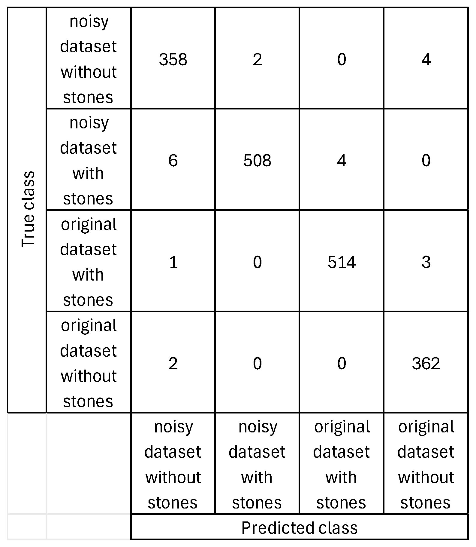
Figure 8 shows the obtained confusion matrix based on the classification results for our proposed system for the fifth case (the dataset and the dataset with random added noise type). Using these confusion matrix values, performance is further evaluated using error, recall, specificity, precision, false positive rate, F1 score, Matthew’s correlation coefficient, and kappa. The performance parameters values are the following: accuracy of 98.75%, error of 1.25%, recall of 98.77%, specificity of 99.59%, precision of 98.62%, false positive Rate of 0.41%, F1 score of 98.7%, Matthew’s correlation coefficient of 98.28%, and kappa of 96.67%. These performance parameter values indicate a very precise classification of both positive and negative cases, regardless of the conditions of the images in the dataset and the varying properties such as intensity levels, noise, rotation, viewpoint, translation, and lighting.
In order to handle class imbalance, random oversampling was used to balance and test the performance of the proposed system using 2592 images for each label of the four categories. The corresponding obtained ensemble accuracy after balancing is 98.07%.
The proposed model demonstrates high performance on both noisy and original ultrasound data, accurately distinguishing between the presence and absence of kidney stones. This high level of accuracy indicates that the model can be reliable for deployment in real-time ultrasound analysis. Furthermore, its robustness to noise suggests that effective preprocessing techniques or training with augmented/noisy data are needed. As a result, the model holds potential for diagnostic decision support, helping to reduce false positives and missed detections in kidney stone classification for ultrasound images.
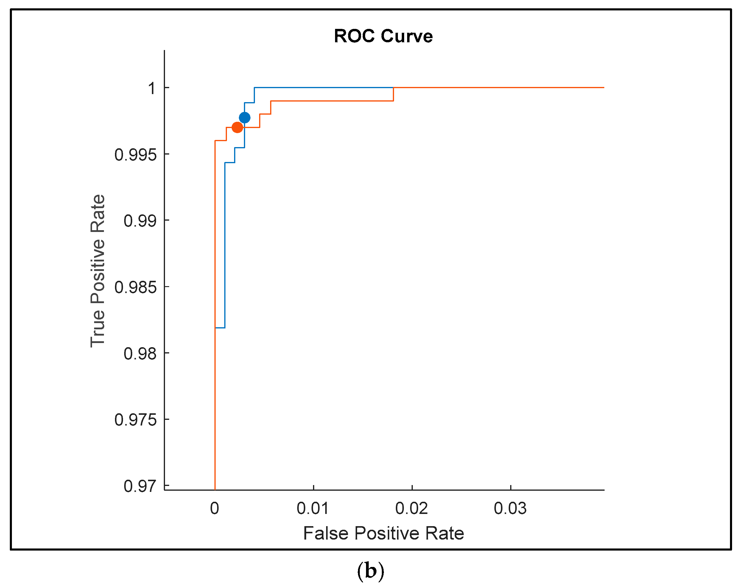
The receiver operating characteristic (ROC) curves shown in
Figure 9 for the classification results of ultrasound images with added random noise (Gaussian, Poisson, speckle, and salt and pepper) provide an insightful comparison of the performance of three deep learning models: Darknet19, InceptionV3, and Darknet53. These curves reflect each model’s ability to distinguish between different classes under noisy conditions, where robustness is critical.
The ROC curve for Darknet19 shows good performance, with the curve quickly rising to the top-left corner of the plot, indicating a very low false positive rate and a high true positive rate. However, the smoothness of the curve suggests fewer threshold variations, likely due to the model’s relatively simpler architecture. The model achieves a true positive rate very close to 1 and a false positive rate close to 0.02, which demonstrates good discrimination even with added noise, but it is not as refined as more advanced networks. The area under the curve (AUC) appears high (close to 0.99), confirming the model’s general effectiveness, though perhaps with slightly reduced flexibility under more complex noise distributions.
InceptionV3, as expected, delivers the most refined and stable ROC curve. It consistently shows high true positive rates across a broader range of false positive thresholds. The curve’s smooth, tight progression toward the top-left corner with minimal deviation indicates a high level of confidence and robustness in classification, even when images are corrupted with complex noise types. The closeness to the upper-left corner and the tightly packed steps suggest fine granularity in decision thresholds and minimal misclassification. The AUC for InceptionV3 likely approaches 1.0, confirming its generalization capabilities and adaptability to noisy medical images. This performance affirms InceptionV3’s advantage in deep feature extraction and noise resilience.
Darknet53 also exhibits high performance, with a steep rise and a curve hugging the top-left axis, very similar to InceptionV3. However, slight deviations and reduced step smoothness suggest a marginally lower precision or slightly higher variability in classification under noise. The curve still maintains a high true positive rate and nearly negligible false positives. It performs better than Darknet19 and nearly matches InceptionV3, showing that its deeper architecture allows for better feature representation and better handling of noise. The AUC is again very high, close to 1.0, indicating a high classification reliability.
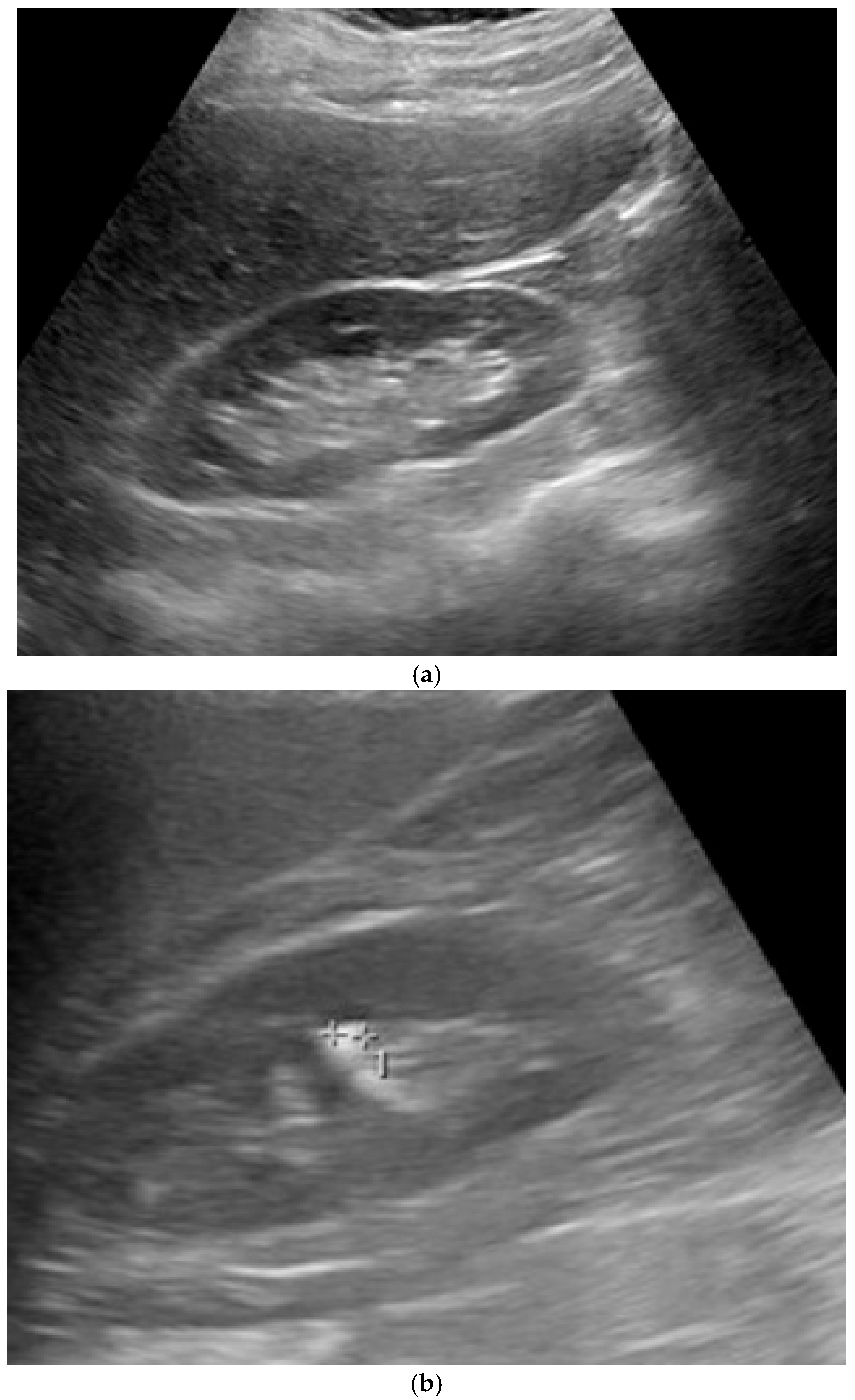
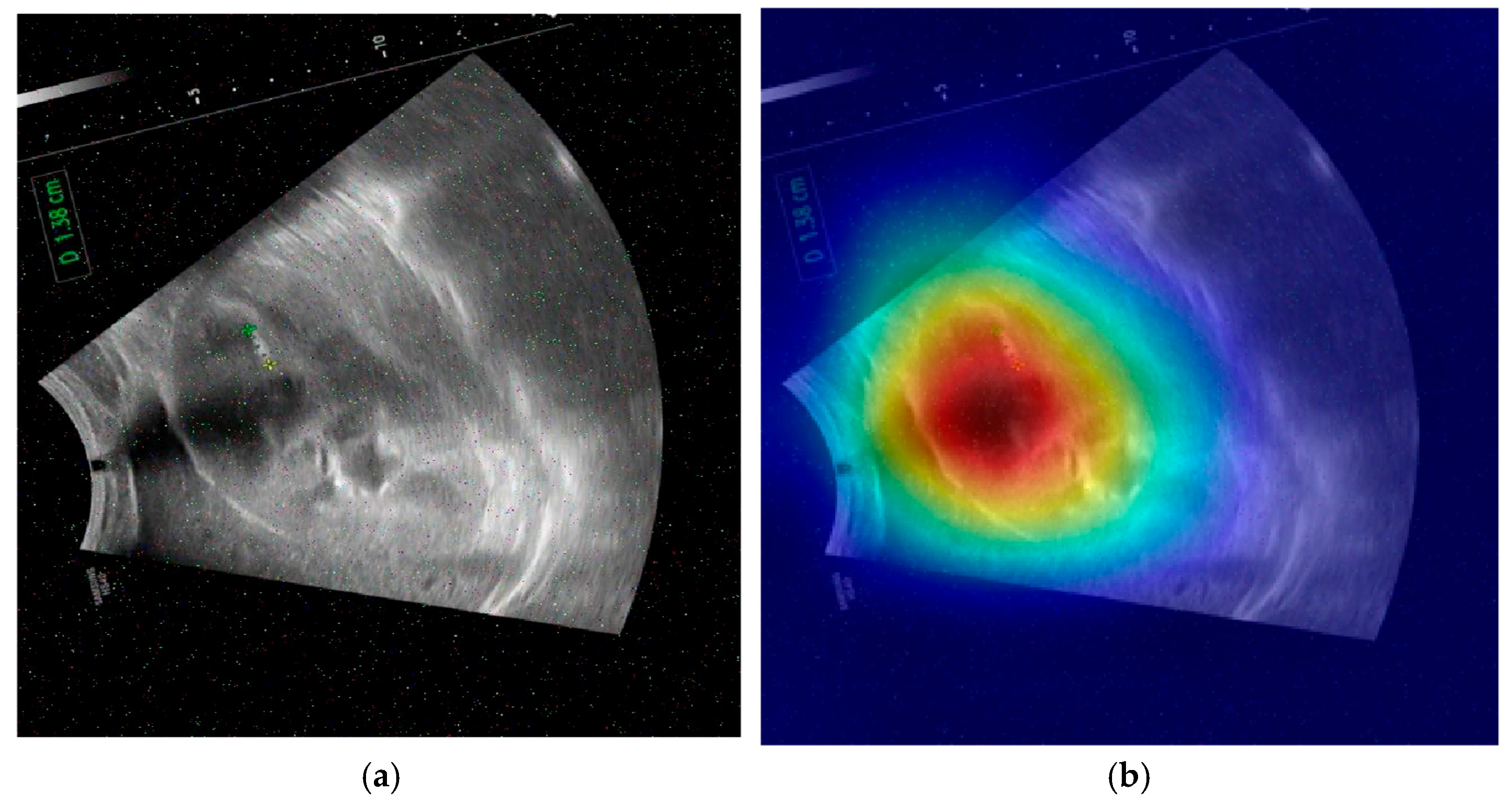
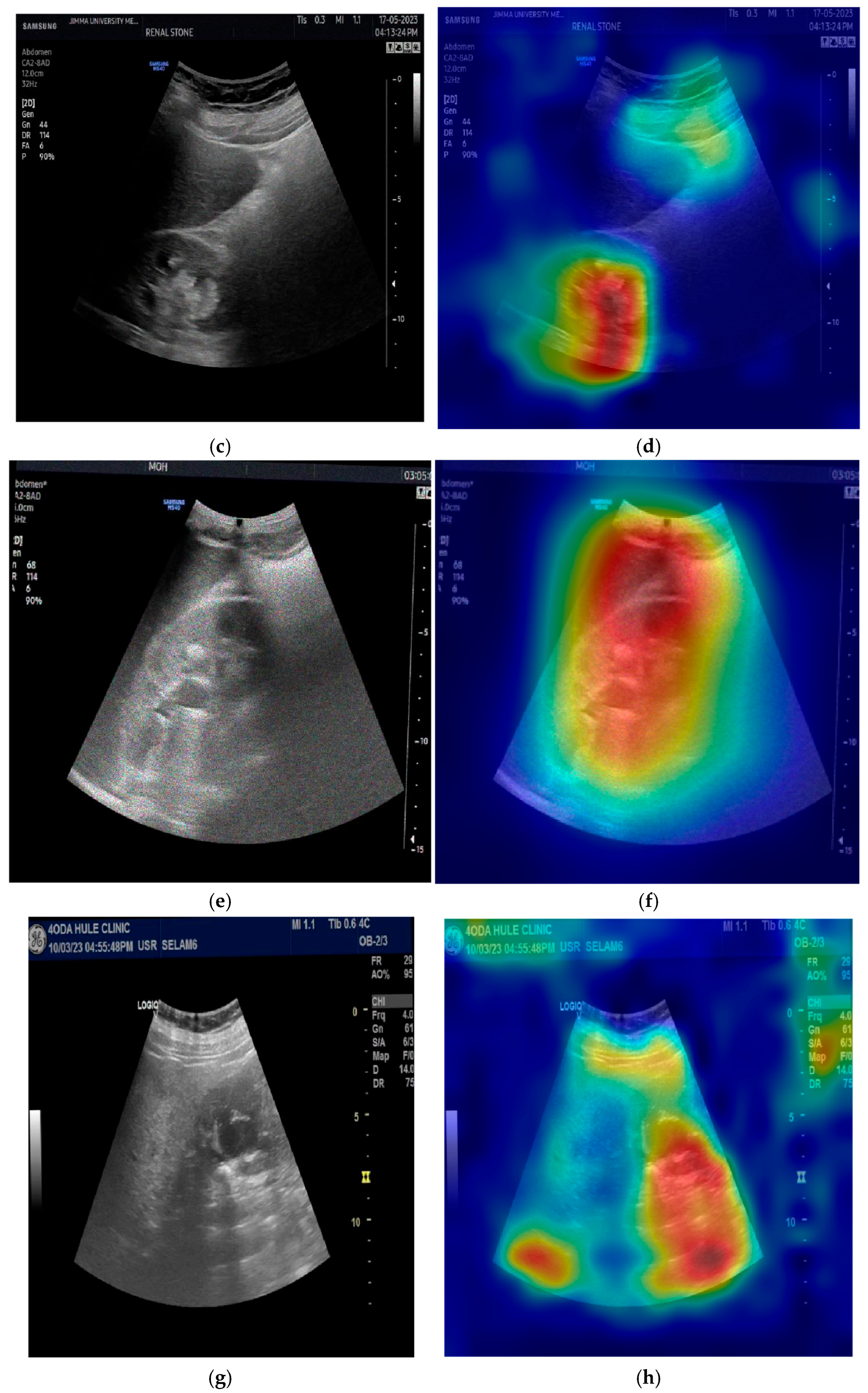
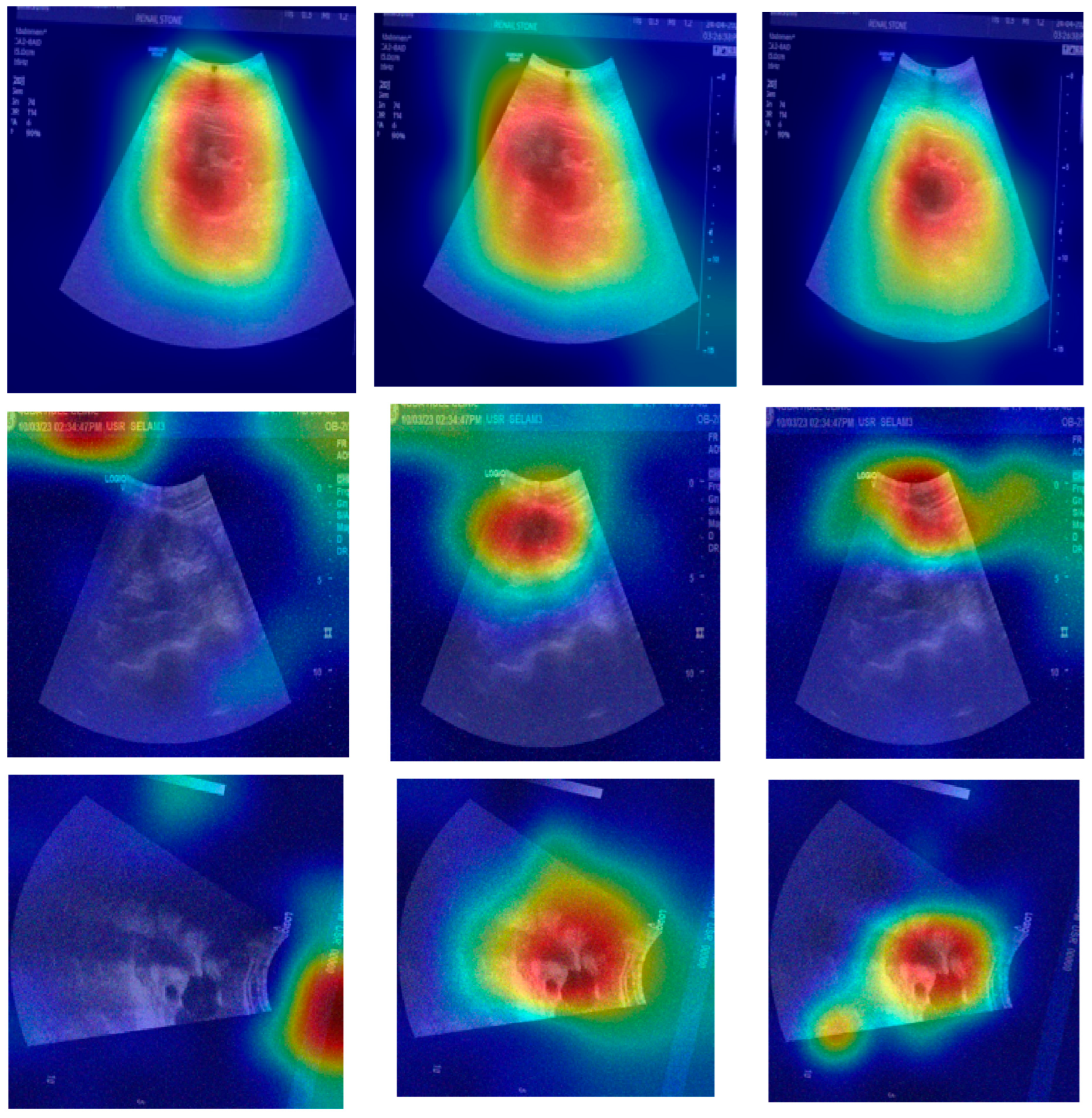
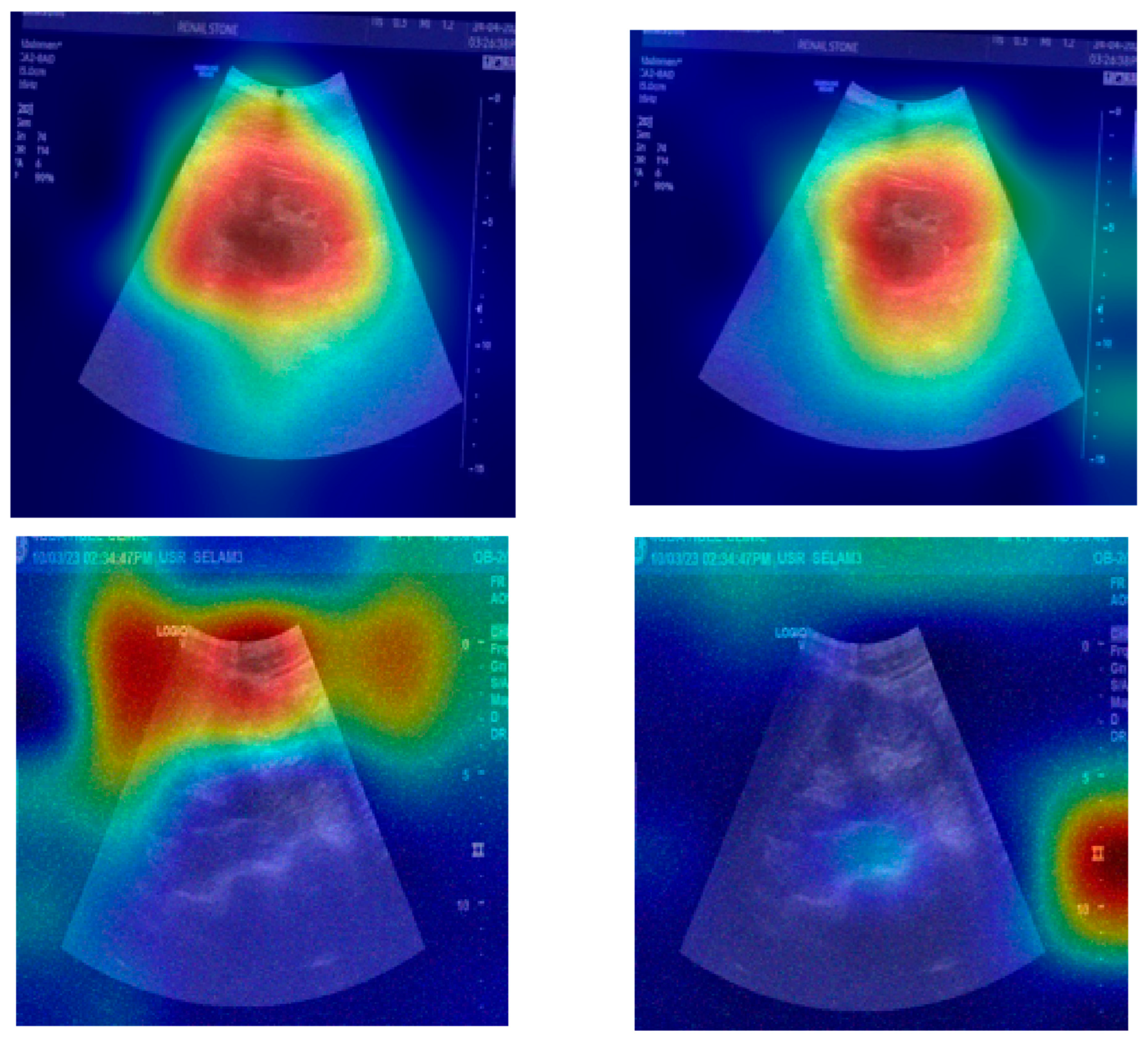
The provided set of images in
Figure 10 displays ultrasound scans of kidneys, with each grayscale image accompanied by the Grad-CAM (Gradient-weighted Class Activation Mapping) visualization. These overlays are commonly used in deep learning to highlight the regions of the image that contributed most to a model’s classification decision. In the medical domain, such tools are essential for interpreting how and why a neural network reaches a particular diagnosis, especially in scenarios like renal stone detection.
Figure 10a shows a standard grayscale ultrasound of a kidney. A noticeable hyperechoic (brighter) area can be seen, which is suggestive of a renal stone. These stones typically appear as bright echoes with posterior acoustic shadowing due to their dense composition. This clinical presentation aligns with what radiologists expect when diagnosing urolithiasis using ultrasound imaging. The corresponding Grad-CAM visualization in the top-right panel overlays a heatmap on this image, where the most intense red zone aligns with the suspected stone. The model focuses its attention on the suspicious region, which suggests that its prediction is based on clinically relevant features. This alignment between the model’s attention and medically significant structures enhances the interpretability and trustworthiness of the AI system.
Figure 10c presents another kidney ultrasound in a different orientation. This image also shows a dense echogenic area near the center, again raising suspicion of a renal stone. The structure’s location and appearance suggest a calculus located near the renal pelvis. The corresponding Grad-CAM map indicates that the deep learning model directs its attention to this same region, evidenced by the red coloration on the heatmap. This correlation between the model’s highlighted region and the likely pathology indicates that the neural network is learning to focus on diagnostically meaningful cues rather than spurious patterns or background noise.
These images and their Grad-CAM overlays demonstrate a level of model interpretability. The deep learning system appears to attend to the correct anatomical regions, those most relevant for diagnosing renal stones. This is vital not only for performance but also for clinical acceptance. Physicians need to understand and trust the reasoning behind automated classifications, especially in healthcare settings.
The visualizations suggest that the model has learned to focus on clinical features, such as echogenic foci and their acoustic shadows, which are indicative of renal stones. This demonstrates the potential for AI-assisted diagnosis in medical imaging.
The proposed method was tested on another dataset in [
50]. That other dataset contains 2776 kidney stone ultrasound images and 2161 normal kidney ultrasound images sourced from low- to mid-range clinical portable units (Philips Lumify and Clarius) used in academic ultrasound labs. The depth varied between 6 cm and 14 cm, with common settings around 10 cm. The dataset included standard renal protocol views (transverse and longitudinal) and some oblique and angled views.
The total number of images was 9874, with random-added noise. Based on the classification results using the proposed ensemble method, the obtained accuracy value with the dataset in [
50] was 98.38%.
The proposed method outperforms existing DNNs in [
24,
25,
26,
27,
28,
29]. Moreover, it also outperforms other recent approaches related to detecting kidney stones on ultrasound images [
33,
34,
35,
36,
37], achieving a classification accuracy of 99.43% on high-quality images (the original dataset images) and 99.21% on the original dataset images with added noise. The method achieved a maximum classification accuracy of 98.75% on the original dataset, besides the original dataset with added noise images (four total classes, the fifth case).
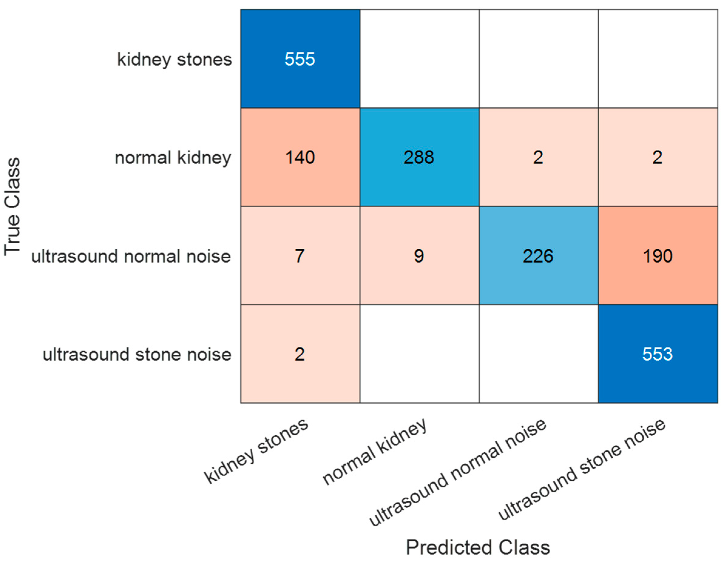
The method was compared with ViTs. ViTs have emerged as a transformative approach in the field of computer vision, offering an alternative to traditional CNNs. Originally developed for natural language processing, the transformer architecture has been adapted to visual tasks by treating images as sequences of patches, similar to tokens in text. The confusion matrix shown in
Figure 11 represents the classification performance of a ViT model on the dataset, in addition to the dataset with the added noise. Ultrasound images categorized under ultrasound normal noise posed a significant challenge for the model. While 226 images were correctly classified, 190 were misclassified as ultrasound stone noise. This indicates that the ViT model struggles to differentiate between noise-induced artifacts in healthy tissue and actual pathological signs, possibly due to the subtlety of differences under distortion. Based on the confusion matrix, the obtained accuracy value is 82.17%.
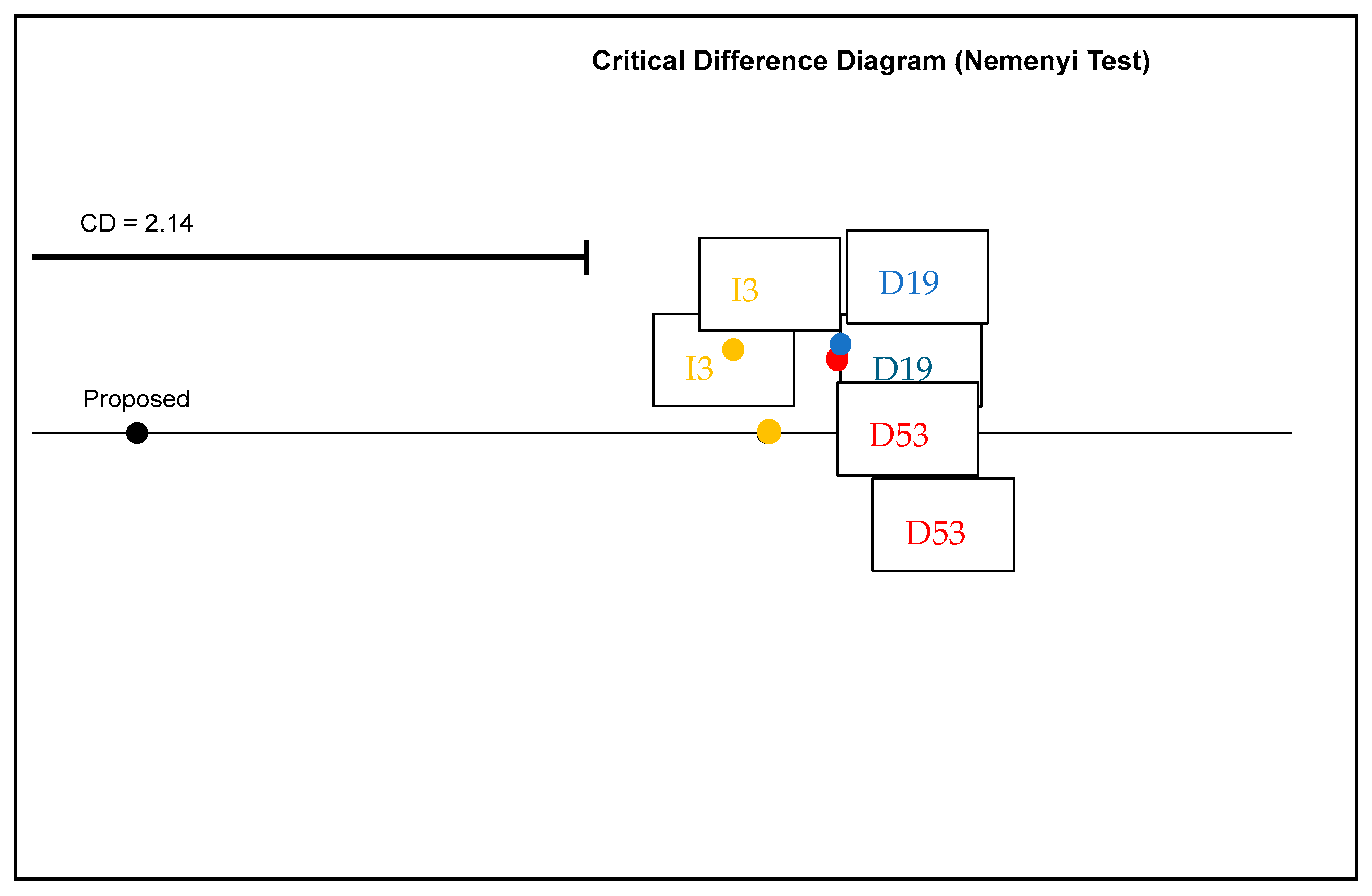
Figure 12 represents a critical difference diagram generated using the Nemenyi post hoc test, which is applied to statistically compare multiple classifiers over multiple datasets. This helps in determining whether the differences in average performance rankings are statistically significant.
The models were benchmarked using the critical difference diagram, as shown in
Figure 12: the proposed model, InceptionV3 (I3), Darknet19 (D19), and Darknet53 (D53). They were plotted along a horizontal axis according to their average rank, with lower ranks (left side) indicating a better performance. The proposed model was placed furthest to the left, suggesting it had the best average rank and thus performed best overall across the tested datasets. I3, D19, and D53 were positioned to the right of the proposed model, indicating a comparatively lower performance.
The critical difference (CD) is specified as 2.14. This value represents the minimum difference in average rank required for the performance between two models to be considered statistically significant at a certain confidence level (α = 0.05). In this case, the distance between the proposed model and the other models (I3, D19, and D53) appears to exceed the CD threshold, indicating that the proposed model is statistically significantly better than I3, D19, and D59.
This conclusion is strengthened by the fact that no connecting line joins the proposed model to I3, D19, or D59, suggesting that the Nemenyi test identified a significant difference between their ranks. Consequently, the diagram supports the claim that the proposed model not only performed high in terms of average rank but also this is statistically validated.
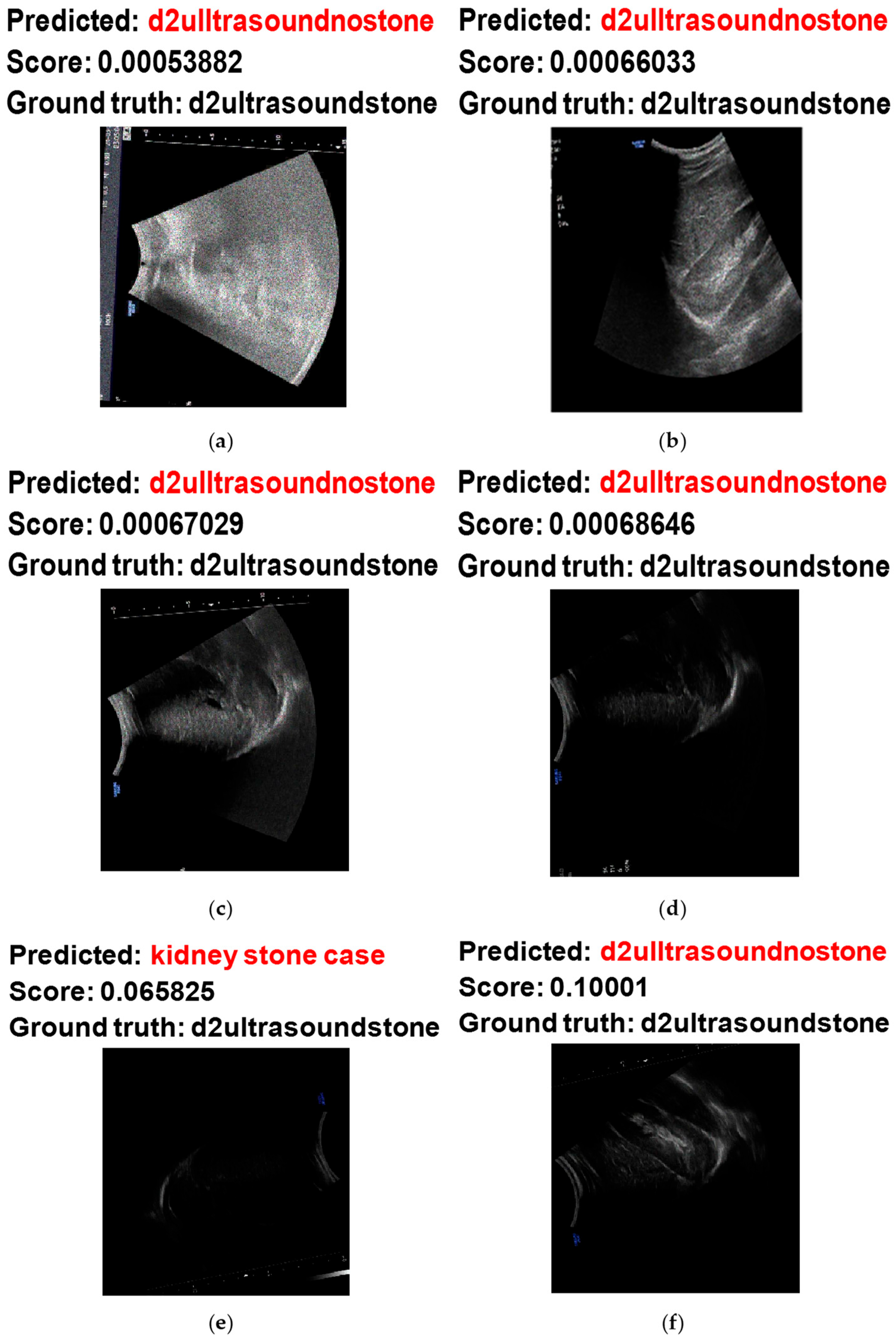
Figure 13 shows some examples of the hardest images to classify when using the proposed system. Based on
Figure 13a,b, the model misclassified the noisy ultrasound images with stones as noisy ultrasound images without stones. This misclassification occurred on these images because of the high concentration of noisy pixels, which made the classification challenging. On the other hand, the misclassification of
Figure 13c,d occurred due to low image intensity from the scan, making it difficult to obtain useful and visual features to decide.
Figure 13e,f shows the misclassification of noisy ultrasound images with stones as noisy images without stones. These two images also have low intensity values from the scanning.
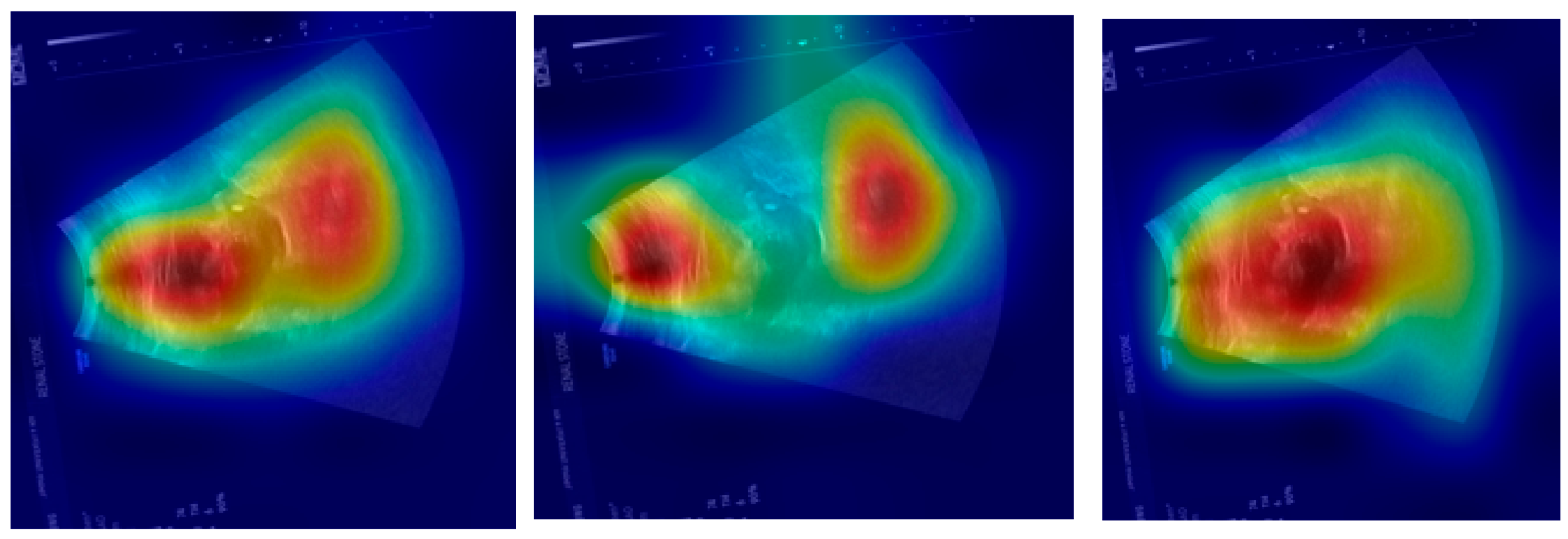
Figure 14,
Figure 15 and
Figure 16 show Grad-CAM visualizations to compare interpretability across different models. In
Figure 14, AlexNet highlights outer regions in the first, second, and third image examples. Darknet faces some difficulties in highlighting relevant regions in the second image. In
Figure 15, EfficientNet points at some outer regions in the second and third image examples. Googlenet maps outer regions with lower focus in the second, third, and fourth example images. Shufflenet highlights outer regions with a lower focus in the second image case. In
Figure 16, both ResNet and Mobilenet show a high focus on outer regions in the second image.
Table 2 shows the obtained FP and FN cases based on the results in
Figure 8. Based on the analysis of the confusion matrix with class-specific labeling, the model’s performance varies across different types of conditions. The original dataset with stones is the most accurately classified class. It has the lowest overall error rate of 1.52%, indicating that the model has a very high confidence and accuracy when predicting this class. The false positive rate for this class is only 0.44%, and the false negative rate is 0.77%, reflecting that the model seldom misses actual cases belonging to it.
The noisy dataset without stones has the highest error rate at 4.00%, which is significantly higher than the others. This class also shows the highest false negative rate (1.65%), which means the model often misses identifying true samples from this category. Additionally, the false positive rate is 0.85%, which contributes to the overall difficulty the model faces when distinguishing this noisy negative class from others.
The noisy dataset with stones performs well, with a false positive rate of only 0.22%, the lowest among all classes, which means that very few samples from other classes are incorrectly classified as noisy stone images. However, its false negative rate is 1.93%, the highest among all classes, indicating the model sometimes fails to recognize true positive instances from this group. This leads to a total error rate of 2.30%.
The original dataset without stones has a low false negative rate of 0.55% and a false positive rate of 0.66%. Its total error rate stands at 2.42%, placing it better than the noisy negative class but behind the original dataset with stones in terms of overall reliability.
The model performs best when dealing with non-noisy data, especially the original dataset with stones, and struggles more when distinguishing noisy non-stone images, likely due to the visual similarities introduced by noise.
The presented performance comparison tables (
Table 3 and
Table 4) evaluate various kidney image classification techniques, offering critical insights into the evolution of medical image analysis methodologies.
Table 3 presents a comprehensive comparison that encompasses both traditional machine learning approaches and deep learning methods, while
Table 4 focuses specifically on deep neural network architectures. These tables collectively demonstrate advancements in classification accuracy, robustness to noise, and the impact of dataset scale on model performance.
Table 3 reveals progression in classification accuracy from traditional machine learning techniques to modern deep learning approaches. The earliest methods ([
33,
34]) utilizing K-nearest neighbors (KNNs) and support vector machines (SVMs) achieve modest accuracies of 56.35% and 64.04%, respectively. These conventional methods, while computationally efficient, are limited by their reliance on handcrafted features and struggle with the complex patterns in medical imaging. The inclusion of meta-heuristic optimization in [
34] provides a marginal improvement, highlighting the challenges of traditional computer vision techniques in medical image analysis.
The transition to deep learning marks a significant leap in performance, with [
35]’s off-the-shelf CNN features achieving 92.31% accuracy. This substantial improvement underscores the power of learned feature representations over manual feature engineering. The ensemble MSVM model in [
36] shows an anomaly; its performance slightly improves (from 84.89% to 85.15%) with added noise, suggesting potential inherent regularization effects or robustness in the ensemble structure. The work by Zheng et al. [
37] demonstrates the value of combining traditional texture features with deep learning, achieving 91.73% accuracy despite using a relatively small dataset of 270 images.
Recent advancements are particularly noteworthy. Sudharson and Kokil’s [
51] ensemble deep neural network achieved 96.54% accuracy, while Asaye et al.’s [
52] machine learning approach reached 98.4%. These results highlight the benefits of sophisticated model architecture and careful feature engineering. The proposed ensemble method, combining Darknet19, Darknet53, and InceptionV3, sets a new benchmark with 99.43% accuracy and maintains 98.75% performance under noisy conditions. This exceptional performance can be attributed to several factors: the strengths of the constituent models, comprehensive noise augmentation during training (including salt and pepper, speckle, Poisson, and Gaussian noise), and the substantial training dataset of 8826 images, nearly double the size of most comparative studies.
Table 4 provides a focused comparison of deep learning architectures, all evaluated on the same dataset size (4940 images) except for the proposed method. The performance spectrum reveals important architectural insights. SqueezeNet [
25] achieves the lowest accuracy (72.31%), demonstrating the challenges of maintaining performance with extreme model compression. InceptionV1 (GoogLeNet) [
24] shows 86.73% accuracy, while ResNet [
26] and ShuffleNet [
28] perform notably better at 93.46% and 93.65%, respectively, illustrating the benefits of residual connections and efficient channel shuffling operations.
The proposed method’s 98.75% accuracy outperforms these established architectures, despite using the same evaluation framework. This stems from some aspects: the ensemble approach leverages Darknet19’s efficiency, Darknet53’s depth and feature extraction capabilities, and InceptionV3’s multi-scale processing. The comprehensive noise augmentation strategy during training (employing multiple noise types with random variances) has enhanced the model’s robustness, as evidenced by its performance in
Table 3’s noise-added scenario.
The progression from traditional methods to deep learning, and further to ensemble approaches, demonstrates a clear evolution in medical image analysis. Several key observations emerge:
Dataset size impact: The correlation between dataset size and performance is evident, though not absolute. While [
51] achieves 96.54% with 4940 images, the proposed method’s larger dataset (8826 images) emphasizes the importance of data scale in deep learning to maximize testing on numerous cases.
Noise robustness: The proposed method’s minimal accuracy drops (0.68%) under noisy conditions compared to other techniques demonstrates the effectiveness of its multi-noise augmentation strategy. This is particularly valuable for medical imaging, where acquisition artifacts are common.
Architectural aspect: The ensemble approach capitalizes on complementary model strengths, Darknet’s object detection capabilities combined with Inception’s multi-scale processing. This synergy explains the significant performance leap over individual architecture.
While high accuracy is promising, the real test lies in clinical deployment. The method’s robustness to various noise types suggests a good generalization potential.
Several areas warrant further investigation, such as the ensemble’s computational requirements versus its performance benefits, the potential for knowledge distillation to reduce model size while maintaining accuracy, extension to other medical imaging modalities, and a detailed analysis of false positive/negative rates in clinical scenarios.
Table 5 presents a comparison between the proposed ensemble deep learning model and some widely used existing deep neural networks on the same dataset (original images and the images with added random noise types).
The proposed ensemble model achieves an accuracy of 98.75%. This result clearly illustrates the strength of using an ensemble approach combining Darknet53, Darknet19, and InceptionnetV3, where the combined predictions of multiple models lead to more robust and accurate outcomes. Specifically, Darknet53 contributes deep hierarchical features, Darknet19 provides lightweight and fast inference capabilities, and InceptionNetV3 brings multi-scale feature extraction.
Conventional CNNs like AlexNet perform low (78.34%), primarily due to their shallow architecture and limited capacity to model complex patterns in noisy data. More modern models like GoogLeNet and ResNet50/101 show improved results, with accuracies ranging from 87.89% to 90.61%, yet they still fall short of the proposed method. ResNet18 achieves 94.39%, outperforming its deeper variants, which might indicate better generalization or less overfitting on this dataset. EfficientnetB0 and MobileNet V2, which are designed for performance–efficiency trade-offs, result in accuracy of 92.49% and 91.55%, respectively, though still not matching the ensemble’s accuracy.
Newer and more powerful models, such as Swin, showed a high performance with an accuracy that is close to the proposed system’s accuracy (97.79%), while ConvNext did not demonstrate a high performance (33.07%).
The results underscore the unique value of ensemble learning, combining Darknet53, Darknet19, and InceptionnetV3 in medical image analysis, especially for challenging data like ultrasound. While single models may perform well in isolation, they often have specific weaknesses, such as susceptibility to noise or difficulty capturing certain patterns, that can be mitigated through model fusion. In clinical settings, even small gains in accuracy can translate to significant improvements in diagnostic confidence and patient care. Therefore, the proposed ensemble model’s performance (98.75%) makes it a candidate for integration into computer-aided diagnostic tools for kidney disease detection via ultrasound.
The study in [
53] presents a lightweight, real-time capable object detection model for thyroid nodules. It builds upon the YOLOv8 framework by integrating a Coordinate Attention-based C2fA module and custom loss functions to improve accuracy. The authors report improvements in mean average precision, reaching 43.6%, with a detection precision of 54% and recall of 58.2%. The model also achieves fast inference times of approximately 7.7 milliseconds per image, which is advantageous for real-time clinical settings.
In comparison, the proposed study focuses on the classification of kidney ultrasound images under both clean and noisy conditions using an ensemble of Darknet19, Darknet53, and Inceptionv3. This ensemble approach achieves a higher classification accuracy of 98.75%. Performance metrics derived from confusion matrices, such as recall (98.77%), specificity (99.59%), F1 score (98.7%), and kappa (96.67%), indicate superior classification reliability. These results suggest that the kidney ultrasound system provides a highly accurate identification of pathological conditions, even in the presence of noise.
In terms of computational efficiency, the two approaches diverge. The study in [
53] is designed for speed and resource efficiency, making it suitable for real-time applications in clinical settings. Its compact architecture and optimized design yield fast inference times and minimal computational overhead. On the other hand, the kidney classification system employs an ensemble of heavier networks, which results in increased time consumption. While exact timing benchmarks are not reported, the use of three deep models suggests a trade-off: the model favors high accuracy and noise robustness over real-time performance.
Noise handling is a key strength of our study. The study in [
53] focuses on enhancing detection performance under natural conditions without explicitly introducing noise. Our study applied four distinct types of noise with randomly selected variances to simulate imaging degradations. This testing under noisy conditions demonstrates the proposed model’s strong resilience to various artifacts in ultrasound imaging. The minimal performance degradation confirms the model’s robustness.
Regarding interpretability, our study leverages Grad-CAM to visualize regions in ultrasound images that influence the model’s predictions. This helps ensure clinical relevance by demonstrating that the model focuses on diagnostically important regions, such as echogenic kidney stones. These visualizations enhance transparency and can build trust with medical practitioners. In contrast, the YOLOv8-based thyroid detection model does not incorporate explicit interpretability tools, such as attention maps or Grad-CAM, which limits its transparency.
Both models offer valuable contributions tailored to different clinical needs. The study in [
53] focuses on fast and efficient thyroid nodule detection and shows improvements in precision and recall with architectural enhancements. Our study demonstrates a high classification performance and resilience to various noise types, supported by Grad-CAM. While it may demand more computational resources, its robustness and clinical transparency make it highly suitable for diagnostic decision support systems in environments where noise is a significant challenge.
Each approach reflects a different priority: the study in [
53] focuses on real-time detection and architectural efficiency, while our study emphasizes accuracy, robustness, and interpretability in classification tasks. These differences underline the complementary nature of the two studies in advancing the state of medical image analysis using deep learning.


