Geo-Statistics and Deep Learning-Based Algorithm Design for Real-Time Bus Geo-Location and Arrival Time Estimation Features with Load Resiliency Capacity

Abstract

This paper introduces a groundbreaking decentralized approach for real-time bus monitoring and geo-location, leveraging advanced geo-statistical and multivariate statistical methods. The proposed long short-term memory (LSTM) model predicts bus arrival times with confidence intervals and reconstructs missing positioning data, offering cities an accurate, resource-efficient tracking solution within typical infrastructure limits. By employing decentralized data processing, our system significantly reduces network traffic and computational load, enabling data sharing and sophisticated analysis. Utilizing the Haversine formula, the system estimates pessimistic and optimistic arrival times, providing real-time updates and enhancing the accuracy of bus tracking. Our innovative approach optimizes real-time bus tracking and arrival time estimation, ensuring robust performance under varying traffic conditions. This research demonstrates the potential of integrating advanced statistical techniques with decentralized computing to revolutionize public transit systems.

1. Introduction

The rapid advancement of intelligent transportation systems (ITSs) has revolutionized urban mobility, particularly in the domain of public transit. Real-time bus monitoring and geo-location prediction have emerged as critical components in enhancing the efficiency, reliability, and user experience of public transportation systems. Recent studies have demonstrated significant progress through the integration of machine learning, deep learning, and real-time data analytics. For instance, Ouyang et al. [1] proposed a long short-term memory (LSTM) based model incorporating historical and real-time data for passenger flow prediction as in [2], achieving superior accuracy compared to traditional methods. Similarly, Yuan et al. [3] developed a deep feature extraction framework using Recurrent Neural Networks (RNNs) and Deep Neural Networks (DNNs) to predict dynamic bus travel times, outperforming conventional machine learning models by 4.82%. Despite these advancements, existing approaches often rely on centralized architectures that can lead to high computational loads, network congestion, and delays in processing large-scale spatiotemporal data. To address these limitations, this paper introduces a groundbreaking decentralized approach for real-time bus monitoring and geo-location, leveraging advanced geo-statistical and multivariate statistical methods. Our system significantly reduces network traffic and computational overhead by decentralizing data processing, enabling data sharing and sophisticated analysis across distributed nodes.

A key innovation of our approach lies in its ability to estimate pessimistic and optimistic arrival times using the Haversine formula, providing real-time updates that enhance the accuracy of bus tracking under varying traffic conditions. This method ensures robust performance even in scenarios with incomplete or sparse GPS data, a common challenge in urban environments. By integrating advanced statistical techniques with decentralized computing, our system optimizes real-time bus tracking and arrival time prediction [4,5], offering a scalable and efficient solution for modern public transit systems. This research builds upon prior works, such as those conducted by Yin et al. [6], who constructed prediction intervals for bus travel times based on road segment sharing and multiple routes’ driving style similarity, and Rashvand et al. [7], who utilized neural networks for real-time bus departure prediction with an accuracy of under 80 s deviation. However, unlike these centralized models, our decentralized framework addresses the scalability and latency issues inherent in traditional systems, paving the way for a new generation of ITS solutions. The remainder of this paper is organized as follows: Section 2 reviews related works in real-time bus monitoring and geo-location prediction. Section 3 details the methodology and architecture of our decentralized system. Section 4 presents experimental results and performance evaluations. Finally, Section 5 concludes the paper and outlines future research directions.

2. Literature Review

The field of intelligent transportation systems (ITSs) has seen significant advancements in recent years, particularly in areas such as passenger flow prediction, bus travel time prediction, and location-based services. These advancements are driven by the integration of big data analytics, deep learning models, and real-time data processing techniques. Recent studies highlight the evolving landscape of Mobility as a Service (MaaS) in Italy, emphasizing both practical implementations and theoretical frameworks. The paper [8] presents empirical insights from pilot studies across diverse Italian regions, demonstrating how MaaS integration can influence user behavior and system scalability. Complementing this, the paper [9] proposes a sustainable MaaS (S-MaaS) framework, integrating transport system models with sustainability goals to guide future urban mobility planning. Together, these works underscore the importance of combining real-world experimentation with robust methodological foundations to advance MaaS adoption and its alignment with environmental and societal objectives.

2.1. Passenger Flow Prediction

Ouyang et al. [1] introduced an LSTM-based method that considers both historical and real-time data for passenger flow prediction. Their model incorporates feature extraction using Xgboost, information coding based on historical and real-time data, and decoding through a multi-layer neural network. The authors claim their approach achieves better accuracy compared to traditional LSTM and other baseline methods. Similarly, Yuan et al. [3] developed a deep feature extraction framework combining Recurrent Neural Networks (RNNs) and Deep Neural Networks (DNNs) for dynamic bus travel time prediction, while [10] used fixed-wing UAV. Their method uses spatiotemporal characteristics and attention mechanisms, achieving a 4.82% improvement over traditional machine learning models.

2.2. Travel Time and Location Prediction

In the realm of travel time prediction, Yin et al. [6,11] proposed a model based on road segment sharing, multiple routes’ driving style similarity, and the bootstrap method. This approach constructs prediction intervals for bus travel times, demonstrating better quality when using fused datasets from multiple routes. Meanwhile, Rashvand et al. [7] leveraged neural networks for real-time bus departure prediction, achieving an accuracy of under 80 s deviation, which significantly improves reliability in smart IoT public transit applications. Location prediction has also advanced with the use of deep learning techniques. Xiao et al. [12,13,14] proposed a hybrid LSTM neural network for vehicle location prediction, effectively reducing trajectory information loss and improving prediction accuracy. Nawaz et al. [15] addressed GPS trajectory completion using a bidirectional convolutional recurrent encoder-decoder architecture with an attention mechanism, which outperformed state-of-the-art benchmark methods.

2.3. Optimization and Scheduling

Yu et al. [16] focused on optimizing urban bus network scheduling by integrating passenger waiting and onboard times into a synchronous optimization model as in [17]. They demonstrated that this approach reduces passenger time costs by 21.5% and operational costs by 13.7%. Rosca et al. [18] designed a Public Urban Transport Scheduling System (PUTSS) using artificial intelligence to allocate fleets based on real-time passenger counts and congestion levels, achieving a global accuracy rate of 89.81%.

2.4. Challenges and Future Directions

While significant progress has been made in transportation modeling, several critical challenges remain unresolved. First, while existing systems increasingly incorporate real-time data, their robustness and scalability under diverse environmental conditions require further enhancement. Second, current models typically rely on predictable patterns, leaving them vulnerable to sudden disruptions; developing more adaptive frameworks capable of handling anomalies is essential. Additionally, the predominant focus on single-mode transportation systems presents limitations—integrating multi-modal data could yield more holistic insights and significantly improve overall network efficiency. With the push toward sustainable cities, optimizing energy consumption in transportation systems remains an open challenge that warrants further investigation. Spatial navigation systems often struggle to adapt in real time to unpredictable urban conditions, such as sudden traffic congestion, extreme weather, or accidents. For example, flooding or road closures can render precomputed routes obsolete. Effective navigation requires integrating live traffic sensors, weather forecasts, and crowd-sourced data to dynamically reroute passengers while balancing efficiency and safety.

3. Material and Methods

This chapter outlines the materials and methodologies employed in our study. We begin by describing the datasets used, including their sources, preprocessing steps, and key features. Next, we present the mathematical models for distance calculation and arrival time estimation, detailing their theoretical foundations and implementation. Finally, we introduce the neural network architecture—specifically, the LSTM-based framework—highlighting its design choices, hyperparameters, and training process. Together, these components form the basis for our experimental analysis and results. A mathematical notation overview is reported in the Appendix D.

3.1. Bus Activity Management Software Components

The Operational Support System (OSS) serves as the backbone of fleet management, providing real-time vehicle tracking, performance diagnostics, and driver assistance through onboard telematics and IoT sensors. The Passenger Information System (PIS) delivers dynamic, multi-channel updates to riders, including live arrival predictions, service alerts, and personalized journey planning via mobile apps and digital displays. Finally, the Network Planning System (NPS) optimizes routes, schedules, and resource allocation using predictive analytics and demand modeling, ensuring efficient long-term transit network design. Together, these integrated systems enable data-driven transportation management while improving both operator workflows and the passenger experience.

3.2. Bus Data Collector

To ensure continuous learning, the bus system will gather data every minute. Specifically, it retrieves the $k^{th}$ measurement’s minute $m^{\left(k\right)}$, hour ($h^{\left(k\right)}$), and day of the week ($d^{\left(k\right)}$) from the local OSS server, along with the start station ($i^{\left(k\right)}$), stop station ($j^{\left(k\right)}$), bus speed ($s^{\left(k\right)}$), and corresponding latitude (${\varphi }^{\left(k\right)}$) and longitude (${\lambda }^{\left(k\right)}$). This steady flow of information enables constant analysis and adaptation. Ultimately, the dataset ${\mathbb{D}}_N$ is built, comprising N observations recorded at hour h and between the specified start and stop stations.

$${\mathbb{D}}_N=\left\{(d^{\left(k\right)},h^{\left(k\right)},m^{\left(k\right)},s^{\left(k\right)};i^{\left(k\right)},j^{\left(k\right)},{\varphi }^{\left(k\right)},{\lambda }^{\left(k\right)});k=1\dots N\right\}$$

(1)

3.2.1. Dataset Descriptive Statistics

Table 1. Dataset descriptive statistics overview table.

Statistic	Speed (km/h)	Latitude	Longitude
Mean	19.160920	34.245540	−6.552059
Standard Deviation	10.979964	0.007078	0.006190
Minimum	0.000000	34.234180	−6.562787
Maximum	33.500000	34.257655	−6.542176

presents descriptive statistics for the latitude, longitude, and speed features. It summarizes key statistical measures such as mean, standard deviation, minimum, and maximum values for these attributes, offering a comprehensive overview of their distribution and variability within Appendix A.

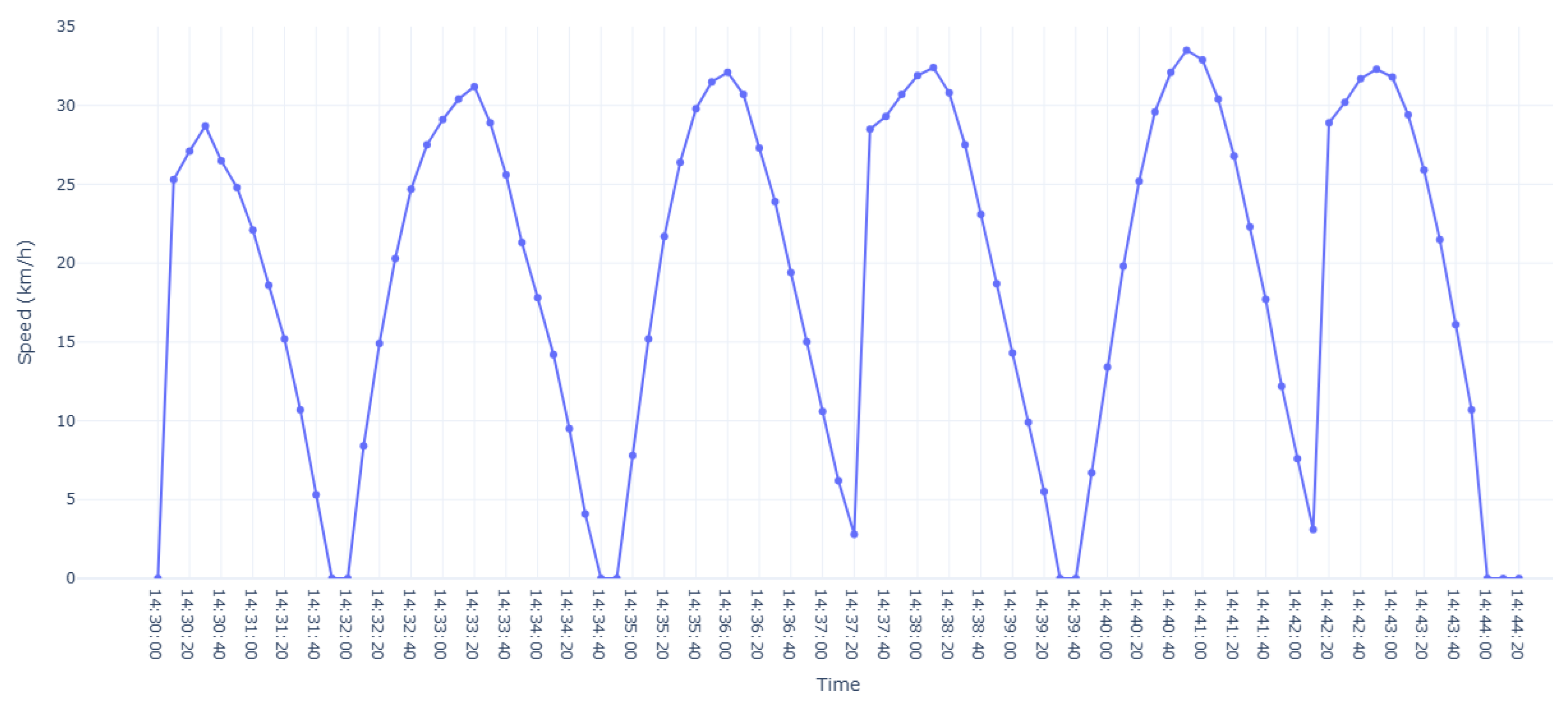
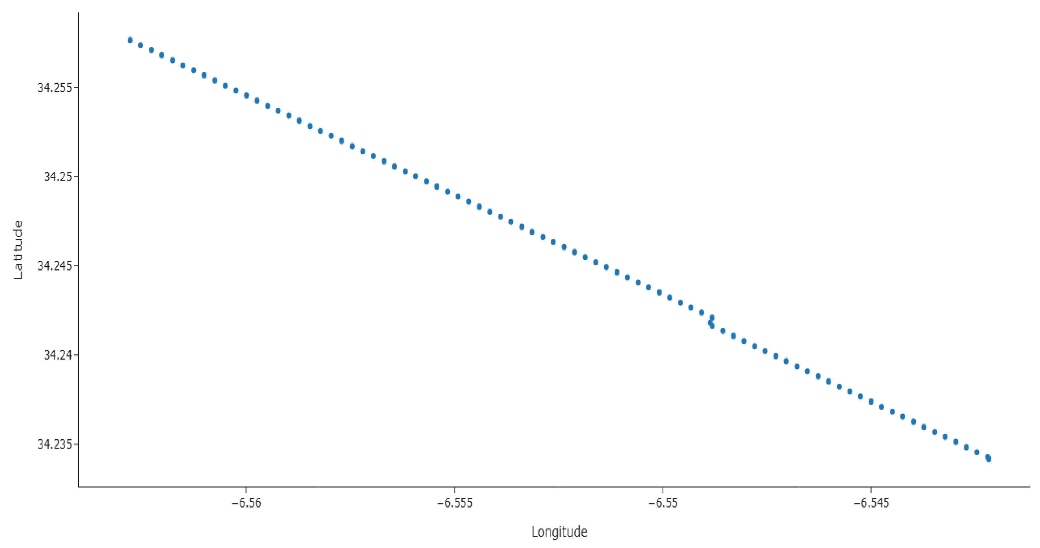
3.2.2. Data Visualization

Figure 1 illustrates the evolution of the bus speed over time during the 15 min test line. The plot highlights periods of acceleration, deceleration, and two complete stops (speed = 0 km/h), reflecting realistic traffic conditions including congestion and scheduled pauses. Speed variations are aligned with the bus’s positional data, demonstrating smooth transitions before and after stops.

Figure 2 shows the topology on the latitude/longitude plane, highlighting spatial distributions, where the sizes of the points are proportional to the speed. The diagonal distribution reflects the primary route’s orientation in the urban grid, which follows a northeast–southwest corridor due to the city’s layout. Appendix C shows the topology in a 2D map for better visualization.

Figure 3 illustrates a front-view visualization of the 3D topology. It provides a clear representation—seen from the front or back perspective—of the structure and arrangement of the dataset’s morphological features, enabling a detailed analysis of its topology.

Figure 4 illustrates a left–right view visualization of the 3D topology. It provides a clear representation—seen from the left or right perspective.

3.3. Speed Confidence Interval Estimation

In this section, we detail the process of modeling bus speed by calculating the average speed for each hour of the day and subsequently constructing confidence intervals to quantify the uncertainty associated with these average speed estimates.

3.3.1. Average and Variance Speed Calculation

To begin, we categorize the speed data based on the hour. This entails grouping all speed measurements recorded within the same hour of the day. For each hour, the average speed is calculated, represented as $\overline{S}(h,d)$, using the formula:

$$\overline{S}(h,d)={\displaystyle \frac{1}{n_h}}\sum _{k=1}^{n_h}{s}^{\left(k\right)}$$

(2)

Here, $n_h$ denotes the total number of speed observations during hour h, and $s_k$ refers to the individual speed measurements recorded within that hour. This calculated average speed, $\overline{S}(h,d)$, provides an estimate of the typical bus speed for that specific hour. To evaluate the variability of the speed data around the computed average, we determine the sample variance, $V_h\left(s\right)$, for each hour using the formula:

$$V_h\left(s\right)={\displaystyle \frac{1}{n_h-1}}\sum _{k=1}^{n_h}{(s^{\left(k\right)}-\overline{S}(h,d))}^2$$

(3)

The sample variance, $V_h\left(s\right)$, measures the dispersion of the data. Following this, the standard error of the mean, $SE(h,d)$, is derived using the formula:

$$SE(h,d)=\sqrt{{\displaystyle \frac{V_h\left(s\right)}{n_h}}}$$

(4)

The standard error, $SE(h,d)$, reflects the precision of the estimated mean speed, with a smaller standard error indicating a more accurate estimate.

3.3.2. Confidence Interval Construction

To estimate a plausible range for the true mean speed at each hour, we construct confidence intervals. For small sample sizes ($n_h<30$), we apply the normal distribution to account for the increased uncertainty inherent in smaller datasets. The confidence interval, $I_{SPEED}(h,d)$, is calculated as:

$$I_{SPEED}=\left[\overline{S}(h,d)-Z_{\alpha /2}.SE(h,d),\overline{S}(h,d)+Z_{\alpha /2}.SE(h,d)\right]$$

(5)

where $Z_{\alpha /2}$ is the critical Z-value from the normal distribution corresponding to a confidence level of $1-\alpha$ (e.g., $Z=1.96$ for a 95% confidence level). The confidence interval, $CI(h,d)$, provides a range within which the true mean speed for hour h and day d between two stations is likely to lie. A smaller sample size increases the interval’s width, reflecting greater uncertainty in the estimate.

3.3.3. Remaining Time to Arrival Estimation

While standard GIS tools can calculate distances between geographic coordinates in urban environments, this approach creates dependencies on external third-party systems. Our framework offers flexibility by supporting both approaches—users may either integrate with existing GIS solutions or utilize our internal distance computation system, which we describe in detail in the following section.

At the time of prediction, the system receives the bus’s current latitude ${\varphi }_1$ and longitude ${\lambda }_2$, along with the destination station’s latitude ${\varphi }_2$ and longitude ${\lambda }_2$. To accurately estimate the remaining travel time, we compute the great-circle distance between these two points using the Haversine formula. This formula accounts for the Earth’s curvature, providing a more precise distance calculation than simple Euclidean distance, especially for longer routes. The computed distance, along with the bus’s current speed and historical traffic data, will be used to refine the estimated time of arrival. The Haversine formula calculates the great-circle distance between two points on a sphere:

$$d=2rarcsin\left(\sqrt{{sin}^2\left({\displaystyle \frac{\Delta \varphi }{2}}\right)+cos\left({\varphi }_1\right)cos\left({\varphi }_2\right){sin}^2\left({\displaystyle \frac{\Delta \lambda }{2}}\right)}\right)$$

(6)

In this context, d represents the distance between the two points, while r is the Earth’s radius, approximately 6371 km. The variables ${\varphi }_1$ and ${\varphi }_2$ denote the latitudes of the two points, and ${\lambda }_1$ and ${\lambda }_2$ correspond to their respective longitudes. Additionally, $\Delta \varphi$ and $\Delta \lambda$ are defined as the differences in latitude (${\varphi }_2-{\varphi }_1$) and longitude (${\lambda }_2-{\lambda }_1$), respectively.

Given that the time to do a distance is the speed time, the distance is divided by the time, so the confidence interval of the arrival times, combining Equations (5) and (6), is given by Equation (7) below:

$$I_{TIME}=\left[{\displaystyle \frac{d}{\overline{S}(h,d)-Z_{\alpha /2}.SE(h,d)}},{\displaystyle \frac{d}{\overline{S}(h,d)+Z_{\alpha /2}.SE(h,d)}}\right]$$

(7)

3.4. Cost-Effective LSTM-Based Predictive Geo-Location Approach

To ensure efficient server utilization and avoid overloading the system with continuous geo-location data, we implemented a data transmission strategy combined with a reconstruction framework based on time series models. This section outlines the approach in detail.

3.4.1. Data Transmission Protocol

Each bus in the network transmits its speed and geo-location data, including latitude measurement time, ($\varphi$) and longitude ($\lambda$), for a duration of five minutes, followed by a five-minute pause during which no data are sent. This intermittent transmission strategy significantly reduces server load while ensuring sufficient data are available for analysis. In this case, we generate synthetic data—as presented in Appendix A—to simulate the transmission protocol. This synthetic dataset simulates the movement of a bus in Kenitra, Morocco, over 15 min, with measurements taken every 10 s. It includes four columns: timestamp for time-stamped entries, latitude and longitude for geospatial coordinates simulating the bus’s route, and ‘speed’ representing the bus’s velocity, varying between 10 and 50 km/h to emulate realistic fluctuations. The dataset consists of 120 rows, capturing realistic temporal and spatial patterns for predictive modeling. It is designed to train an LSTM model for forecasting the next 5 min speed and location, with the first 5 min serving as training data and the second for validation.

3.4.2. Reconstruction of Missing Data with LSTM Network

The missing data for the five-minute transmission gaps are reconstructed using an (LSTM) neural network. LSTMs are highly effective for this purpose due to their ability to model temporal dependencies and capture non-linear patterns in sequential data. The (LSTM) model is designed to predict two key outputs: latitude and longitude. Its architecture includes a single LSTM layer with 50 units, which captures temporal dependencies within the data, followed by a dense output layer with three units. These output units correspond to the three predicted values: speed, latitude, and longitude. The model is compiled using the Adam optimizer for efficient training and Mean Squared Error (MSE) as the loss function to minimize prediction errors. The input data for the model is organized into sequences derived from the five-minute intervals during which data are actively collected. Each sequence contains time-series data for speed (s), latitude ($\varphi$), and longitude ($\lambda$), ensuring that all features are adequately represented. The target output for the model includes the predicted values of speed and coordinates for each time step within the missing five-minute intervals. To enhance the model’s performance, the input data is preprocessed and normalized prior to training.

To enable real-time adaptation and integration of new information, the LSTM model incorporates an online learning framework. As new data batches are received from the buses, the model is updated incrementally through a training process. This involves reshaping the new input data into the required format, training the model for one epoch with each batch, and validating its performance using historical data. This process ensures the model remains responsive to dynamic changes in the data distribution. During periods where data is missing—such as the five-minute gaps in data transmission—the trained LSTM model predicts the missing speed and geo-location data step-by-step. These predictions are validated against historical records to confirm their reliability. The output from the model provides a reconstructed sequence of speed (s), latitude ($\varphi$), and longitude ($\lambda$), effectively filling in the gaps and enabling continuous monitoring of the buses’ movements.

3.4.3. LSTM Network Settings

Our proposed LSTM network—whose mechanism is explained in Appendix B—exhibits a robust configuration with a total of 4,115,952 parameters, occupying 15.70 MB of memory. All parameters in the network are trainable, ensuring adaptability and optimization during training processes. Notably, the network does not include any non-trainable parameters, thus maximizing its efficiency for the intended tasks. For a comprehensive overview,

Table 2. Latitude and longitude prediction neural network configuration.

Layer (Type)	Output Shape	Params Number
Lstm (LSTM)	(None, 50)	10,800
Dense (Dense)	(None, 1000)	51,000
Dense (Dense)	(None, 1000)	1,001,000
Dense (Dense)	(None, 1000)	1,001,000
Dense (Dense)	(None, 1000)	1,001,000
Dense (Dense)	(None, 1000)	1,001,000
Dense (Dense)	(None, 1000)	1,001,000
Dense (Dense)	(None, 1000)	51,000
Dense (Dense)	(None, 2)	102

below outlines the parameter details, highlighting the memory allocation and structural components of the network.

The structure begins with an LSTM layer (50 units) followed by seven dense layers—five large hidden layers (1000 neurons each) followed by two smaller dense layers (1000 and 2 neurons, respectively). This configuration provides substantial representational capacity, with the final layer’s 2-unit output specifically to predict the latitude and longitude.

Mean Squared Error (MSE) is a metric used to measure the average squared difference between actual and predicted values. It is computed as:

$$\mathrm{MSE}={\displaystyle \frac{1}{n}}\sum _{i=1}^n{(y_i-{\widehat{y}}_i)}^2$$

(8)

where n is the number of data points, $y_i$ is the actual value for the ith data point, and ${\widehat{y}}_i$ is the predict for the ith data point. Within our deep neural network architecture, the ReLU (Rectified Linear Unit) activation function, as referenced in (9), was utilized in both the hidden layers and the output layer. Renowned for its efficiency in deep learning, ReLU introduces non-linearity while addressing the vanishing gradient issue, thereby enhancing the model’s ability to uncover intricate data patterns. By integrating ReLU in the initial layers, the network was enabled to identify and extract a wide array of features effectively.

$$ReLU\left(x\right)=max(0,x)$$

(9)

4. Results and Discussions

This section covers the LSTM model’s training dynamics and validation performance, followed by its practical deployment for real-time bus tracking and arrival prediction in urban networks.

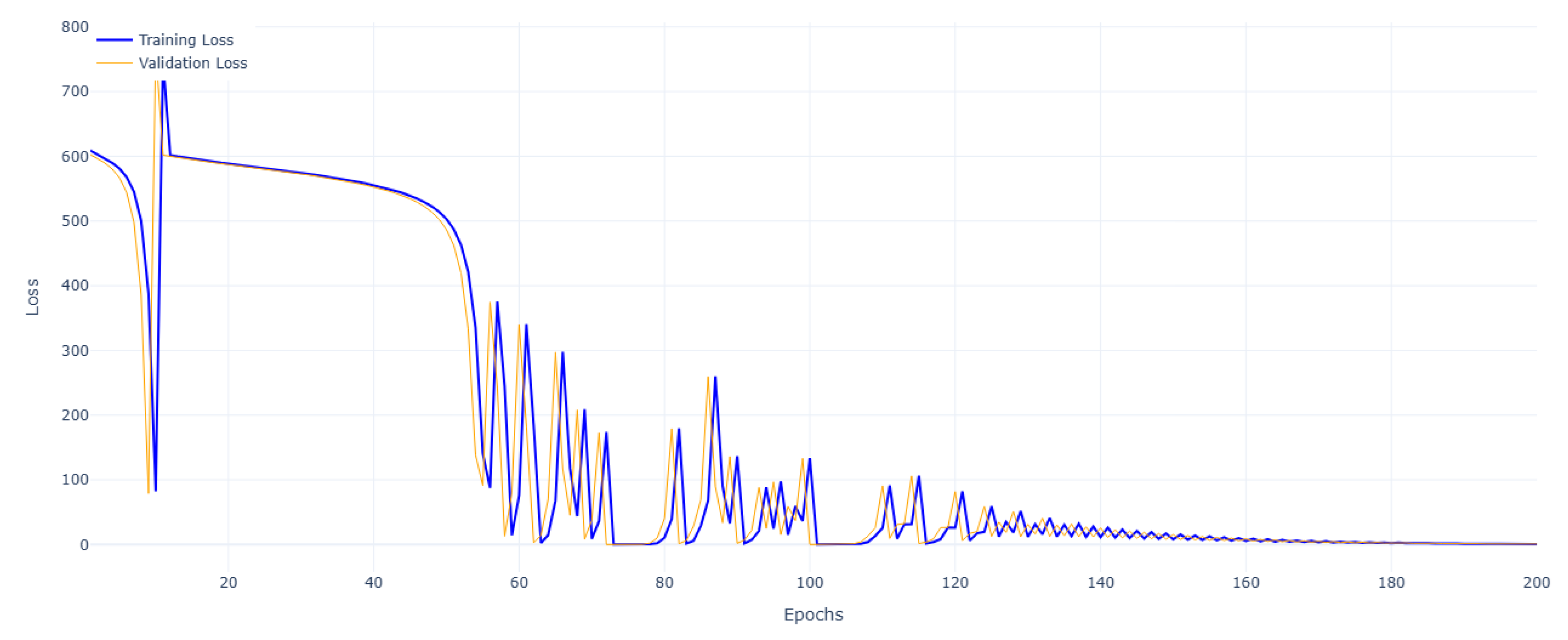
4.1. Network Training and Validation Loss Evolution

The training and validation loss curves in the Figure 5 demonstrate the successful training of the LSTM-based model for real-time bus geo-location and arrival time prediction. It means that the obtained model will allow us to predict the next coordinates and speed based on historical latitude, longitude, and speed data points. Over 200 epochs were used, and both losses rapidly decrease from high initial values (600–700) to near-zero levels, with the training loss stabilizing slightly faster than the validation loss. The close alignment and minimal fluctuations between the two curves indicate strong generalization without significant overfitting, while the logarithmic scale highlights the model’s ability to achieve high precision. Notably, the model converges around 150–200 epochs, reaching optimal performance where it effectively balances learning from the training data and generalizing to unseen validation data. These results underscore the algorithm’s robustness and load resiliency capacity, validating its effectiveness in delivering accurate predictions under varying operational conditions.

4.2. Practical Use of Developments

The practical implementation of our geo-statistics and deep learning hybrid algorithm addresses critical gaps in urban mobility systems through three key functionalities: real-time bus geo-location, arrival time estimation with confidence intervals, and missing data reconstruction. The load-resilient architecture maintains prediction accuracy during variable demand conditions, from low-traffic periods to rush hour congestion.

Transport agencies benefit from enhanced operational visibility, as the system compensates for common GPS signal losses in urban canyons and high-density areas. The geo-statistical components enable spatial analysis of delay patterns, supporting data-driven decisions for route optimization and resource allocation.

Designed for integration with existing telematics infrastructure, the solution provides cities with an upgrade path to advanced predictive capabilities without substantial capital investment. The algorithm’s efficient processing requirements make it suitable for deployment across diverse urban transport networks, from mature smart cities to developing mobility systems.

5. Conclusions and Perspectives

In conclusion, this study presents a transformative decentralized framework for real-time bus geo-location and arrival time estimation, integrating advanced geo-statistical methods, multivariate analysis, and deep learning through LSTM networks. By reducing network traffic and computational overhead via decentralized data processing, the system achieves exceptional scalability and load resiliency. The incorporation of the Haversine formula further enhances accuracy by enabling precise arrival time predictions under diverse traffic conditions. As evidenced by the training and validation results, the model demonstrates robust convergence, generalization, and high predictive performance, validating its suitability for real-world applications. This research underscores the immense potential of combining statistical innovation with decentralized computing to address critical challenges in public transit systems, paving the way for smarter, more efficient urban mobility solutions. One promising direction is the integration of real-time traffic data and weather conditions to further refine arrival time predictions under dynamic urban scenarios. Additionally, exploring federated learning techniques could enhance privacy and data security while maintaining decentralized processing advantages. Expanding the model to multi-modal transportation networks, incorporating metro systems and ride-sharing services, could contribute to a more holistic intelligent transit ecosystem. Finally, investigating the potential of reinforcement learning approaches for adaptive route optimization may further improve the efficiency and responsiveness of public transportation networks.

References

1. Ouyang, Q.; Lv, Y.; Ma, J.; Li, J. An LSTM-Based Method Considering History and Real-Time Data for Passenger Flow Prediction. Appl. Sci. 2020, 10, 3788. [Google Scholar] [CrossRef]
2. Abduljabbar, R.; Dia, H.; Tsai, P.W.; Liyanage, S. Short-Term Traffic Forecasting: An LSTM Network for Spatial-Temporal Speed Prediction. Future Transp. 2021, 1, 21–37. [Google Scholar] [CrossRef]
3. Yuan, Y.; Shao, C.; Cao, Z.; He, Z.; Zhu, C.; Wang, Y.; Jang, V. Bus Dynamic Travel Time Prediction: Using a Deep Feature Extraction Framework Based on RNN and DNN. Electronics 2020, 9, 1876. [Google Scholar] [CrossRef]
4. Lee, C.; Yoon, Y. A Novel Bus Arrival Time Prediction Method Based on Spatio-Temporal Flow Centrality Analysis and Deep Learning. Electronics 2022, 11, 1875. [Google Scholar] [CrossRef]
5. Du, Y.; Wang, C.; Qiao, Y.; Zhao, D.; Guo, W. A geographical location prediction method based on continuous time series Markov model. PLoS ONE 2018, 13, e0207063. [Google Scholar] [CrossRef] [PubMed]
6. Yin, Z.; Wang, B.; Zhang, B.; Shen, X. Prediction Intervals for Bus Travel Time Based on Road Segment Sharing, Multiple Routes’ Driving Style Similarity, and Bootstrap Method. Appl. Sci. 2024, 14, 2935. [Google Scholar] [CrossRef]
7. Rashvand, N.; Hosseini, S.S.; Azarbayjani, M.; Tabkhi, H. Real-Time Bus Departure Prediction Using Neural Networks for Smart IoT Public Bus Transit. IoT 2024, 5, 650–665. [Google Scholar] [CrossRef]
8. Meloni, I.; Musolino, G.; Piras, F.; Rindone, C.; Russo, F.; Sottile, E.; Vitetta, A. Mobility as a Service: Insights from pilot studies across different Italian settings. Transp. Eng. 2024, 18, 100294. [Google Scholar] [CrossRef]
9. Vitetta, A. Sustainable Mobility as a Service: Framework and Transport System Models. Information 2022, 13, 346. [Google Scholar] [CrossRef]
10. Zhou, Y.; Tang, D.; Zhou, H.; Xiang, X. Moving Target Geolocation and Trajectory Prediction Using a Fixed-Wing UAV in Cluttered Environments. Remote Sens. 2025, 17, 969. [Google Scholar] [CrossRef]
11. Chekol, A.G.; Fufa, M.S. A survey on next location prediction techniques, applications, and challenges. EURASIP J. Wirel. Commun. Netw. 2022, 2022, 29. [Google Scholar] [CrossRef]
12. Xiao, Y.; Nian, Q. Vehicle Location Prediction Based on Spatiotemporal Feature Transformation and Hybrid LSTM Neural Network. Information 2020, 11, 84. [Google Scholar] [CrossRef]
13. Song, H.Y. A future location prediction method based on lightweight LSTM with hyperparamater optimization. Sci. Rep. 2023, 13, 17928. [Google Scholar] [CrossRef] [PubMed]
14. Stojković, P.; Tadić, P. Object Location Prediction in Real-time using LSTM Neural Network and Polynomial Regression. arXiv 2023, arXiv:2311.13950. [Google Scholar] [CrossRef]
15. Nawaz, A.; Huang, Z.; Wang, S.; Akbar, A.; AlSalman, H.; Gumaei, A. GPS Trajectory Completion Using End-to-End Bidirectional Convolutional Recurrent Encoder-Decoder Architecture with Attention Mechanism. Sensors 2020, 20, 5143. [Google Scholar] [CrossRef] [PubMed]
16. Yu, X.; Cao, H.; Cao, K.; Zou, L.; Zhu, L. Considering the Optimization Design of Urban Bus Network Scheduling. Appl. Sci. 2024, 14, 6337. [Google Scholar] [CrossRef]
17. Gemma, A.; Cipriani, E.; Crisalli, U.; Mannini, L.; Petrelli, M. A Bus Network Design Model under Demand Variation: A Case Study of the Management of Rome’s Bus Network. Sustainability 2024, 16, 803. [Google Scholar] [CrossRef]
18. Rosca, C.M.; Stancu, A.; Neculaiu, C.F.; Gortoescu, I.A. Designing and Implementing a Public Urban Transport Scheduling System Based on Artificial Intelligence for Smart Cities. Appl. Sci. 2024, 14, 8861. [Google Scholar] [CrossRef]
Figure 1. Speed evolution over time.
Ai 06 00142 g001
Figure 2. Dataset topology visualization on latitude/longitude plan.
Ai 06 00142 g002
Figure 3. Front-view dataset 3D topology visualization.
Ai 06 00142 g003
Figure 4. Left-right-view dataset 3D topology visualization.
Ai 06 00142 g004
Figure 5. LSTM neural network training and validation loss evolution over epochs.
Ai 06 00142 g005