LineMVGNN: Anti-Money Laundering with Line-Graph-Assisted Multi-View Graph Neural Networks

Abstract

Anti-money laundering (AML) systems are important for protecting the global economy. However, conventional rule-based methods rely on domain knowledge, leading to suboptimal accuracy and a lack of scalability. Graph neural networks (GNNs) for digraphs (directed graphs) can be applied to transaction graphs and capture suspicious transactions or accounts. However, most spectral GNNs do not naturally support multi-dimensional edge features, lack interpretability due to edge modifications, and have limited scalability owing to their spectral nature. Conversely, most spatial methods may not capture the money flow well. Therefore, in this work, we propose LineMVGNN (Line-Graph-Assisted Multi-View Graph Neural Network), a novel spatial method that considers payment and receipt transactions. Specifically, the LineMVGNN model extends a lightweight MVGNN module, which performs two-way message passing between nodes in a transaction graph. Additionally, LineMVGNN incorporates a line graph view of the original transaction graph to enhance the propagation of transaction information. We conduct experiments on two real-world account-based transaction datasets: the Ethereum phishing transaction network dataset and a financial payment transaction dataset from one of our industry partners. The results show that our proposed method outperforms state-of-the-art methods, reflecting the effectiveness of money laundering detection with line-graph-assisted multi-view graph learning. We also discuss scalability, adversarial robustness, and regulatory considerations of our proposed method.

1. Introduction

Money laundering is the process of disguising the origins of illegally obtained funds to make them appear legitimate. Existing anti-money laundering (AML) systems can be generally categorized into two groups: rule-based methods and machine learning-based methods. Rule-based methods are popular among commercial institutions due to simple and easy-to-code rules predefined by domain experts [1]. However, it is time-consuming and labor-intensive to keep updating the rules under ever-evolving data. Machine learning-based anti-money laundering (AML) systems leverage large volumes of historical transaction data to learn models. For instance, support vector machine, logistic regression, k-means clustering, k-nearest neighbors, random forests, MLP, etc. [2]. In recent years, graph neural networks (GNNs) have emerged as the de facto tool for graph learning tasks. Example application domains of GNNs for fraud detection tasks include credit card transactions, e-payment data, and cryptocurrency transactions [3].

Some GNNs for digraphs (directed graphs) are suitable for money laundering detection tasks since transaction graphs are directed. However, some not naturally supporting edge features are unsuitable for node-and-edge-attributed transaction graphs. This type of graph is common for account-based transaction graphs, in which nodes and edges represent accounts and transactions, respectively.

Recent state-of-the-art (SOTA) GNNs for digraphs can be categorized into spectral methods [4,5,6,7,8,9,10] and spatial methods [11,12,13]. Spectral GNNs perform graph convolutions by applying graph signal filters in the spectral domain, while spatial GNNs aggregate feature information from neighboring nodes directly in the spatial domain.

Although most of the recent works focus on the spectral methods, spectral GNNs for digraphs may not be suitable for attributed account-based transaction graphs, because (1) they do not naturally support multi-dimensional edge features, and (2) they have limited scalability due to their spectral nature. Usually, full graph propagation is needed during training, and the number of required graph propagations depends on the degree of the polynomial graph filter.

In contrast, spatial GNNs for digraphs may be more suitable for transaction graphs due to the nature of being attributed and directed. However, there is a lack of exploration of spatial GNNs for digraphs. Several relevant papers did not empirically validate the extension of GNNs to digraphs [13,14,15], and some do not apply to transaction graphs due to different reasons, such as graph structural constraints [12], or aggregation from only out-neighbors [13]. Dir-GNN [11] is a generic spatial digraph GNN framework, but the use of separate sets of learnable parameters for in- and out-neighbors may be redundant for some domains such as transaction data. Our experimental results show a good model performance despite parameter sharing. However, we design our models within this framework due to its genericness.

In addition, specifically for AML detection, identifying suspicious accounts by the relevant transactions depends on cash flow information. Nevertheless, such information may not be effectively captured by SOTA GNNs for digraphs such as DiGCN [7], MagNet [6], SigMaNet [5], FaberNet [4], and Dir-GNN [11]. As an illustrative example shown in Figure 1, suppose a series of path-like transactions exist in a transaction graph. The corresponding accounts can be considered suspicious when they serve as temporary repositories for funds [16]. Identifying these suspicious accounts requires identifying suspicious transactions, and identifying a suspicious transaction requires information from (past) receipt and (future) payment transactions, such as comparing the transaction time and the transaction amounts, to acquire the money flow information. Although stacking GNN layers allows information propagation, the edge-to-edge (transaction-to-transaction) information exchange is indirect and less detailed. Also, the first GNN message passing will be meaningless since raw edge (transaction) attributes are aggregated without comparing with other relevant transactions. Early propagation of edge (transaction) information and edge updates before the first iteration of GNN message passing can ease the learning of a GNN model for suspicious account detection.

To capture inter-edge interactions, line graphs of edge adjacencies $L\left(G\right)$ can be leveraged for edge feature propagation. The line graph $L\left(G\right)$ is transformed from the input graph G, where $L\left(G\right)$ encodes the directed edge adjacency structure of G using the non-backtracking matrix, allowing information to propagate along the directed edges while preserving orientation. We propose LineMVGNN which aggregates and propagates transaction information in the line graph before node (account) feature updates in the input graph G.

Our main contributions are as follows:

• MVGNN is introduced as a lightweight yet effective model within the Dir-GNN framework due to its genericness. It supports edge features and considers both in- and out-neighbors in an attributed digraph, such as a transaction graph.
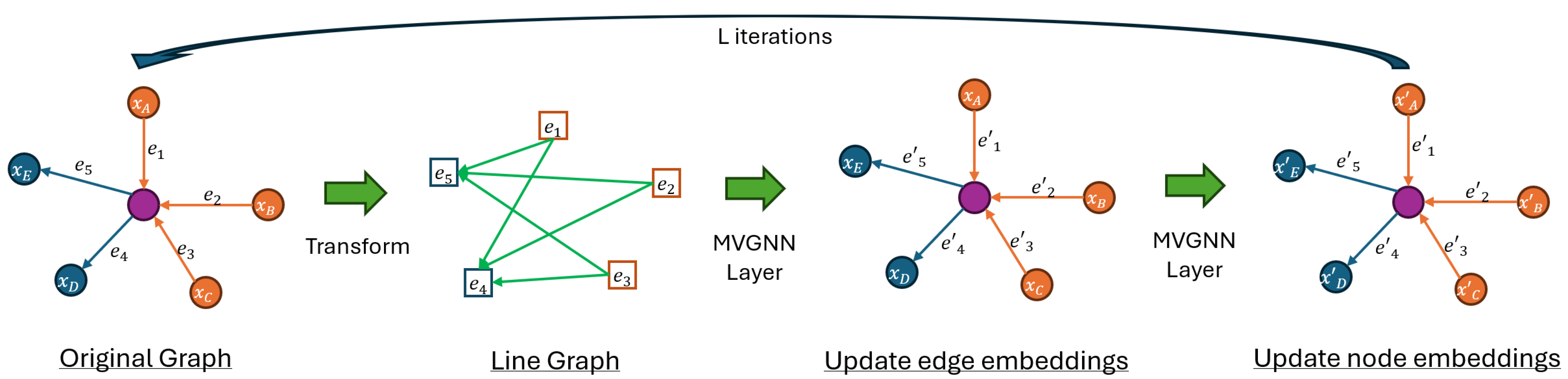
• LineMVGNN is proposed, extending MVGNN by utilizing the line graph view of the original graph for the effective propagation of transaction information (edge features in the original graph).
• Extensive experiments are conducted on the Ethereum phishing transaction network and the financial payment transaction (FPT) dataset.

The remainder of this paper is organized as follows. Section 2 provides an overview of related work in anti-money laundering (AML) and graph neural networks (GNNs) for directed graphs. Section 3 introduces the problem statement and the mathematical framework for our proposed method, including its two-way message passing mechanism and line graph view. Section 4 presents the experimental setup, datasets, and results, comparing LineMVGNN with SOTA methods. Section 5 discusses the limitations of the proposed method and potential future work. Finally, Section 6 concludes the paper with a summary of contributions.

2. Related Work

2.1. GNNs for Digraphs

2.1.1. Spectral Methods

Recently, researchers have extended spectral convolutions to directed graphs [8,9,10]. In particular, DiGCN [7] uses an approximate digraph Laplacian based on personalized PageRank [17] and incorporates kth-order proximity to produce k receptive fields; MagNet [6] utilizes a complex Hermitian matrix, namely the magnetic Laplacian, to encode both undirected structure and directional information; SigMaNet [5] unifies the treatment of undirected and directed graphs with arbitrary edge weights by introducing the Sign-Magnetic Laplacian to extend spectral graph convolution theory to graphs with positive and negative weights; FaberNet [4] utilizes advanced complex analysis and spectral theory to extend spectral convolutions to directed graphs. Nevertheless, spectral GNNs might not be appropriate for edge-attributed transaction graphs, because they do not inherently accommodate multi-dimensional edge characteristics and their scalability is restricted by their spectral characteristics. Typically, full graph propagation is needed during training, with the necessary number of propagations contingent on the degree of the polynomial graph filter.

2.1.2. Spatial Methods

Though the extension of spatial models to directed graphs is suggested in several classical papers, empirical experiments are not conducted [13,14,15]. GGS-NNs [13] handles directed graphs but only aggregates from out-neighbors. It neglects in-neighbor information and edge features. Although DAGNN [12] supports edge features, it is limited to directed acyclic graphs. Extended from the Message Passing Neural Network (MPNN) framework [14], Dir-GNN [11] is a spatial GNN that accounts for edge directionality by separately aggregating messages from in-neighbors and out-neighbors. Although the importance of the two types of messages is differentiated by a hyperparameter, Dir-GNN cannot capture the element-wise interaction between these two types of messages. It also lacks efficiency as it doubles the number of parameters to separately aggregate the two types of messages.

Overall, both spectral and spatial methods fail to effectively address the challenges of transaction-based tasks due to their inability to propagate edge-level information effectively. This limitation is critical for tasks like AML detection, where transaction-level details, such as cash flow patterns, are essential for identifying suspicious activities. Spectral methods are further hindered by their lack of support for multi-dimensional edge features and scalability issues, while spatial methods may struggle to capture nuanced interactions between in- and out-neighbors, leading to inefficiencies and suboptimal performance.

2.2. Edge Feature Learning and Line Graphs

Combining node and edge feature learning has been suggested by some researchers [14,18]. Recently, LGNN [19] operates on line graphs of edge adjacencies, leveraging a non-backtracking operator to enhance performance on community detection tasks. However, the model is restricted to undirected graphs. Multiple works also leverage line graphs for learning edge embeddings, but only for link prediction [20,21].

Although node and edge feature information usually complement each other, edge feature propagation and learning for node classification tasks remain relatively unexplored. To incorporate multi-dimensional edge features for node feature updates, Zhang et al. [22] proposes a graph representation learning framework that generates node embeddings by aggregating local edge embeddings. Nevertheless, the learned edge embeddings do not effectively capture the interactions between edges, since the edge embeddings are learned from the concatenation of the edge features and the features of the corresponding end nodes.

To capture inter-edge interactions and enhance node embeddings, line graphs of edge adjacencies can be leveraged, but this remains relatively unexplored for node classification tasks. CensNet [23] co-embeds nodes and edges by switching their roles using line graphs, but is limited to undirected graphs without parallel edges because of the use of spectral graph convolution. LineGCL [24] transforms the original graph into a line graph to enhance the representation of edge information and facilitate the learning of node features by contrastive learning, but it assumes no edge features in the original graph.

3. Proposed Method

3.1. Problem Statement

Consider a directed transaction graph $G=(\mathcal{V},\mathcal{E})$, where $\mathcal{V}$ is the set of nodes $\{v_1,\dots ,v_n\}$ and $\mathcal{E}$ is the set of edges $\{e_1,\dots ,e_m\}$. Each node represents an account and each edge represents a transaction. An edge’s source node and destination node represent the payer and payee of the corresponding transaction, respectively. Each node v is attributed with $x_v$ and each edge is attributed with $e_{vw}$. Each node is either licit or illicit, and is represented by 0 and 1, respectively. A subset of nodes are unlabeled. We aim to learn a model that predicts the label $y_v$ of each unlabeled node v.

3.2. Two-Way Message Passing

Information from both the in- and out-neighbors and edges is important for node classification. In a digraph, however, messages from the out-neighbors and edges are usually ignored in traditional GNNs such as GCN [25], GraphSAGE [26], GIN [27], etc. In addition, edge attributes are present in some real-world data, and they can be significantly more informative than node attributes. Therefore, we build our simple MVGNN (Multi-View Graph Neural Network) model within the Dir-GNN framework [11]. As illustrated in Figure 2, the model considers messages from both in-neighbors and out-neighbors. Our MVGNN differs from Dir-GNN by (1) parameter sharing between message aggregation functions for in- and out-neighbors, and (2) the message combination function for the two types of messages. Details are provided below.

At the $(l+1)$-th MVGNN layer, aggregation of messages $m_{v_{in}}^{(l+1)}$ and $m_{v_{out}}^{(l+1)}$ can be expressed by the following:

$$\begin{array}{c}\hfill m_{v_{in}}^{(l+1)}=\sum _{w_k\in N_{in}\left(v\right)}{M}_{in}^{(l+1)}\left([h_w^{\left(l\right)}\parallel e_{vw}]\right),\end{array}$$

(1)

$$\begin{array}{c}\hfill m_{v_{out}}^{(l+1)}=\sum _{w_k\in N_{out}\left(v\right)}{M}_{out}^{(l+1)}\left([h_w^{\left(l\right)}\parallel e_{vw}]\right),\end{array}$$

(2)

where $M_{in}^{\left(l\right)}$ and $M_{out}^{\left(l\right)}$ are fully connected layers with ReLU activation, $N_{in}\left(v\right)$ and $N_{out}\left(v\right)$ denote the in- and out-neighbors of node v, $e_{vw}$ denotes the features of an edge between node v and w, and ∥ denotes concatenation.

The node embeddings are updated with these messages by the equation below:

$$h_v^{(l+1)}=U^{(l+1)}\left(h_v^{\left(l\right)},C^{(l+1)}\left(m_{v_{in}}^{(l+1)},m_{v_{out}}^{(l+1)}\right)\right),$$

(3)

where the vertex update function $U^{(l+1)}$ is a fully connected layer with ReLU activation. For the message combination function $C^{(l+1)}$, we experiment with 2 different methods. For brevity and clarity, superscript is omitted, i.e., $C^{(l+1)}$, $m_{v_{in}}^{(l+1)}$, and $m_{v_{out}}^{(l+1)}$ will become C, $m_{v_{in}}$, and $m_{v_{out}}$ respectively.

Combine by Weighted Sum. To differentiate the importance of messages from in-neighbors and out-neighbors, similarly to [11], we propose a variant MVGNN-add, which multiplies weight scalars with $m_{v_{in}}$ and $m_{v_{out}}$:

$$C\left(m_{v_{in}}^{(l+1)},m_{v_{out}}^{(l+1)}\right)={\alpha }_{l+1}{m}_{v_{in}}^{(l+1)}+(1-{\alpha }_{l+1})m_{v_{out}}^{(l+1)},$$

(4)

where ${\alpha }_{l+1}\in \mathbb{R}$ is a learnable scalar (instead of a hyperparameter as in [11]).

Combine by Concatenation. To better model the element-wise interaction between messages from these two types of neighbors, MVGNN-cat is proposed (instead of using weighted sum as in [11]). The two types of messages are concatenated and then passed to a linear layer $F^{(l+1)}$:

$$C\left(m_{v_{in}}^{(l+1)},m_{v_{out}}^{(l+1)}\right)=F^{(l+1)}\left([m_{v_{in}}^{(l+1)}\parallel m_{v_{out}}^{(l+1)}]\right).$$

(5)

To boost model efficiency, we share parameters for aggregation maps, message combination maps, and vertex update functions for both types of neighbors in our experiments. In other words, the primary power of distinguishing between in- and out-messages lies in the learnable parameter $\alpha$, or the linear layer F. In experiments, this proposed model remains competitive.

In short, at a high level, the $(l+1)$-th MVGNN layer can be expressed as follows:

$$h_v^{(l+1)}={\mathrm{MVGNNLayer}}^{(l+1)}\left(\{h_u^{\left(l\right)},h_w^{\left(l\right)},e_{vu}^{\left(l\right)},e_{vw}^{\left(l\right)}|u\in {\mathcal{N}}_{in}\left(v\right),w\in {\mathcal{N}}_{out}\left(v\right)\}\right),$$

(6)

where MVGNNLayer $=\{\mathrm{MVGNNLayer}-\mathrm{add}$, and $\mathrm{MVGNNLayer}-\mathrm{cat}\}$, $e_{vu}^{\left(l\right)}$ and $e_{vw}^{\left(l\right)}$ are edge embeddings. Since there are no edge updates, $e_{vu}^{\left(l\right)}=e_{vu}$ and $e_{vw}^{\left(l\right)}=e_{vw}$. “MVGNNLayer-add” denotes message combination by weighted sum defined in Equation (4), while “MVGNNLayer-cat” denotes message combination by concatenation followed by a linear layer.

To prevent over-smoothing neighbors’ information, similar to [28], personalized PageRank-based aggregation mechanism of GNN [29] is adopted to obtain the final aggregated embedding $z_v$ of node v:

$$\begin{array}{c}\hfill z_v=\sum _{l=1}^{L-1}{\beta }_l{h}_v^{\left(l\right)}+\left(1-\sum _{l=1}^{L-1}{\beta }_l\right)\times h_v^{\left(L\right)},\end{array}$$

(7)

where ${\beta }_l\in \mathbb{R}$ is a learnable parameter. Subsequently, a fully connected layer maps each $z_v$ to a prediction vector $y_v$.

3.3. Line Graph View

Whether a transaction is illicit also depends on the previous transactions due to the significance of the money flow. To facilitate capturing this information, we leverage line graphs to perform edge feature propagation. To the best of our knowledge, few studies have leveraged line graphs in anti-money laundering. One example is LaundroGraph [30] which represents edges as nodes and implements a GNN on the line graph.

The original transaction graph G is transformed into a line graph $G^{\prime }=\mathcal{L}\left(G\right)$, in which each node $t(v,w)\in G^{\prime }$ corresponds to edge $e_{vw}\in G$ (transaction from w to v). In the line graph $G^{\prime }$, a directed edge $e_{t(v,w)t(u,s)}^{\prime }$ exists if $u=w$ (i.e., the payee u of transaction $t(u,s)$ is the payer w of transaction $t(v,w)$).

Figure 3 and Algorithm 1 show how our proposed LineMVGNN leverages the line graph view and propagates edge features. In the line graph $G^{\prime }$, edge feature propagation is performed with $G^{\prime }$ before each message passing in G. LineMVGNN uses separate MVGNN layers for the original graph G and the line graph $G^{\prime }$, respectively, as defined in Equation (6). To seamlessly involve the line graph view in every message passing in the original graph G, inspired by the cross-stitch networks [31], we update the edge features with $G^{\prime }$ before each message propagation in G as shown from line 5 to 7 in Algorithm 1. Residual connection [32] is adopted for edge embedding updates, as shown in line 6. Note that a dummy edge feature [1] can be used for models requiring edge features, which are usually absent in $G^{\prime }$. With the use of line graphs, edge features can be effectively propagated. In other words, information about a particular transaction can be propagated to the next transactions, capturing money flow.

Algorithm 1 LineMVGNN

Input: Graph $G=(\mathcal{V},\mathcal{E})$; input node features $\{h_v^{\left(0\right)},\forall v\in \mathcal{V}\}$; input edge features $\{e_{vw}^{\left(0\right)},\forall v\in \mathcal{V},w\in {\mathcal{N}}_{out}\left(v\right)\}$; model depth L Parameter: $\{{\mathrm{MVGNNLayer}}_G^{\left(l\right)},{\mathrm{MVGNNLayer}}_{G^{\prime }}^{\left(l\right)}\}:\forall l\in L$ Output: Vector $z_v,\forall v\in \mathcal{V}$   1: $G^{\prime }\leftarrow \mathcal{L}\left(G\right)$   2: Initialize in G: $h_v^{\left(0\right)}\leftarrow x_v$.   3: Initialize in $G^{\prime }$: $t_{v,w}^{\left(0\right)}\leftarrow e_{vw}^{\left(0\right)}$.   4: for  $l=0$ to L do   5:     With $t^{\left(l\right)}(v,w)$ in $G^{\prime }$, apply ${\mathrm{MVGNNLayer}}_{G^{\prime }}^{(l+1)}$ and obtain $t^{(l+1)}(v,w)$ by Equation (6).   6:     $e_{vw}^{\left(l\right)}\leftarrow t^{(l+1)}(v,w)$   7:     With $e_{vw}^{\left(l\right)}$ in G, apply ${\mathrm{MVGNNLayer}}_G^{(l+1)}$ and obtain $h_v^{(l+1)}$ by Equation (6).   8: end for   9: $z_v\leftarrow$ Equation (7) 10: return  $z_v$

The LineMVGNN model is further divided into 2 variants: LineMVGNN-add if using weighted sum for combining messages as defined in Equation (4), or LineMVGNN-cat which concatenates message vectors followed by a linear layer as defined in Equation (5).

3.4. Computational Complexity

The overall complexity of this propagation scheme is dominated by the edge propagation on the line graph $G^{\prime }$, which has a complexity of $\mathcal{O}\left(L\right|\mathcal{E}{|}^2)$ for L model layers, and the line graph construction, which has a complexity of $\mathcal{O}\left(\right|\mathcal{E}{|}^2)$ in the worst case, such as in a complete graph. The propagation scheme can be optimized by avoiding explicit line graph construction. Edge propagation can be performed directly on the original graph G, as shown in Algorithm 2. In this refined LineMVGNN, edges in G are treated as first-class entities. For each edge $e_{vw}\forall (v,w)\in \mathcal{E}$, messages are aggregated from neighboring edges that share a common node. With a sparse graph, this reduces the asymptotic computational complexity to $\mathcal{O}\left(L\right|\mathcal{E}\left|\right)$, which is the same with GCN [25].

Algorithm 2 Refined LineMVGNN (Without Explicit Line Graph Construction)

Input: Graph $G=(\mathcal{V},\mathcal{E})$; input node features $\{h_v^{\left(0\right)},\forall v\in \mathcal{V}\}$; input edge features $\{e_{vw},\forall v\in \mathcal{V},w\in {\mathcal{N}}_{out}\left(v\right)\}$; model depth L Parameter: $\{{\mathrm{MVGNNLayer}}_{\mathrm{node}}^{\left(l\right)},{\mathrm{MVGNNLayer}}_{\mathrm{edge}}^{\left(l\right)}\}:\forall l\in L$ Output: Vector $z_v,\forall v\in \mathcal{V}$   1: $h_v^{\left(0\right)}\leftarrow x_v$.   2: for  $l=0$ to  L  do   3:    # Edge Feature Propagation   4:    Scan for $N_{in}\left(e_{vw}\right)$ and $N_{out}\left(e_{vw}\right)$.   5:    $e_{vw}^l\leftarrow$ apply ${\mathrm{MVGNNLayer}}_{\mathrm{edge}}^{\left(l\right)}$ by Equation (6), treating $e_{vw}$ as the first-class entities.   6:    # Node Feature Propagation   7:    Scan for $N_{in}\left(v\right)$ and $N_{out}\left(v\right)$.   8:    $h_v^{(l+1)}\leftarrow$ apply ${\mathrm{MVGNNLayer}}_{\mathrm{node}}^{(l+1)}$ by Equation (6).   9: end for 10: $z_v\leftarrow$ Equation (7) 11: return  $z_v$

4. Experiments

4.1. Datasets

Two datasets are used to evaluate LineMVGNN in the classification of benign nodes against illicit counterparts.

4.1.1. Ethereum (ETH) Datasets

Ethereum Phishing Transaction Network data is a real public transaction graph dataset available on Kaggle. Each node represents an address, and each edge represents a transaction. The nodes are labeled as either phishing or not. Each edge contains two attributes: the balance and the timestamp of the transaction. To address the node class imbalance and huge graph size, we adopt graph sampling strategies similar to [33,34], creating two data subsets with different subgraph sizes, namely ETH-Small (12,484 nodes and 762,443 edges) and ETH-Large (30,757 nodes and 1,298,315 edges). Since no node attributes are provided in the original dataset, we further derive variant data subsets by adding structural node features (SNFs): in-degrees and out-degrees, yielding a total of four data subsets: ETH-Small (w/ SNF), ETH-Large (w/ SNF), ETH-Small (w/o SNF), and ETH-Large (w/o SNF). We adopt a semi-supervised transductive learning setting to classify nodes as illicit (fraud) nodes or benign, and treat all non-central nodes as unlabeled. Nodes of each extracted subgraph are randomly split into training, validation, and test sets at a ratio of 60%:20%:20%.

4.1.2. Financial Payment Transaction (FPT) Dataset

Provided by our industry partner, this transaction dataset contains e-wallet payment transaction data from January 2022. After data preprocessing, a transaction graph is constructed for each day, where accounts and transactions are represented by nodes and edges, respectively. No SNFs are added. As we assume that the real data contain no anomalous money laundering patterns, synthetic anomalies are injected into the graphs, following the injection strategy from [35]. The proportion of illicit (money laundering) nodes constitutes roughly one-third of the total node count. On average, there are 1,048,512 nodes and 1,092,895 edges in the graphs for each day. A supervised transductive learning setting is used to classify nodes as either illicit (money laundering) or benign. The transaction graphs for the whole month are chronologically split into training, validation, and test sets at a ratio of 60%:20%:20%. For more details, please refer to Appendix A.

4.2. Compared Methods and Evaluation Metrics

The following baseline GNNs are compared with our proposed methods: (1) Non-digraph GNNs include GCN [25], GraphSAGE, [26], MPNN [14], GIN [27], PNA [36], and EGAT [37]; (2) Digraph GNNs includes DiGCN [7], MagNet [6], SigMaNet [5], FaberNet [4], and Dir-GCN and Dir-GAT [11].

Since jumping knowledge [38] by concatenation (“cat”) and by max-pooling (“max”) are applied in FaberNet, Dir-GCN, and Dir-GAT, we build the corresponding variant models, namely FaberNet (cat), FaberNet (cat), Dir-GCN (cat), Dir-GCN (max), Dir-GAT (max), and Dir-GAT (cat). For models that do not naturally support edge features, we concatenate them with node features.

Since some datasets are very imbalanced, the F1 score for the illicit class is used for model performance evaluation, which is similar to what is used in real-world scenarios.

4.3. Results

Table 1. F1 scores of the illicit class. For each dataset, the highest F1 score is bold and underlined, and the 1st runner-up is underlined. “OOM” indicates out of memory.

Category	Methods	ETH-Small		ETH-Large		FPT
		w/ SNF	w/o SNF	w/ SNF	w/o SNF	w/o SNF
Non-Digraph GNNs	GCN	0.8770	0.8998	0.9068	0.9072	0.8817
	GraphSAGE	0.8752	0.6705	0.8984	0.6705	0.8802
	MPNN	0.7857	0.8912	0.8854	0.9087	OOM
	GIN	0.9055	0.8954	0.9117	0.8950	0.8802
	PNA	0.9352	0.9105	0.9130	0.9249	OOM
	EGAT	0.8916	0.6705	0.9195	0.6705	OOM
Digraph GNNs	DiGCN	0.8192	0.8055	0.8650	0.8290	OOM
	MagNet	0.9009	0.9012	0.9330	0.9354	0.9616
	SigMaNet	0.8072	0.8319	0.8018	0.8300	0.5033
	FaberNet (cat)	0.9352	0.9393	0.9476	0.9451	0.9934
	FaberNet (max)	0.9336	0.9376	0.9381	0.9460	0.9945
	Dir-GCN (cat)	0.9240	0.8987	0.9168	0.9188	0.6402
	Dir-GCN (max)	0.8577	0.9000	0.8598	0.9207	0.6402
	Dir-GAT (cat)	0.8831	0.6705	0.8769	0.6705	0.9768
	Dir-GAT (max)	0.7958	0.6705	0.8515	0.6705	0.9908
Our Digraph GNNs	MVGNN-add	0.9231	0.9333	0.9300	0.9365	0.9821
	MVGNN-cat	0.9331	0.9301	0.9439	0.9394	0.9858
	LineMVGNN-add	0.9362	0.9407	0.9598	0.9048	0.9905
	LineMVGNN-cat	0.9441	0.9455	0.9394	0.9565	0.9954

summarizes the F1 scores of the illicit class across five datasets for all models. Our LineMVGNN model, especially the variant model LineMVGNN-cat, achieves state-of-the-art results on nearly all datasets.

Compared to non-digraph GNN baselines, LineMVGNN beats the competing methods by an average of 9.68% across all datasets. For each dataset, the improvement is at least 0.89%, 3.50%, 4.03%, 3.16%, and 11.37% on the ETH-Small (w/ SNF), ETH-Small (w/o SNF), ETH-Large (w/ SNF), ETH-Large (w/o SNF), and FPT datasets, respectively. Compared to digraph GNN baselines, LineMVGNN improves the prediction illicit F1 scores by an average of 10.79% across all datasets. For each dataset, the increment is at least 0.89%, 0.62%, 1.22%, 1.05%, and 0.09%, respectively. It is noteworthy that our LineMVGNN model achieves over 99% in the FPT dataset without SNFs. This shows the effectiveness of leveraging both the line graph view and the reverse view for node classification tasks (illicit account detection). In addition, even with shared parameters among GNN aggregation maps for in-neighbors and those for out-neighbors, the performance of our MVGNN variant models matches with other competing digraph GNN methods. This confirms that high model efficiency and expressiveness were achieved.

4.4. Discussion

4.4.1. Effect of Different Views

As shown in

Table 2. Illicit F1 in the ablation experiments. “TWMP” and “LGV” stand for “two-way message passing” and “line graph view”, respectively.

Method	Components	ETH-Small		ETH-Large		FPT
		w/ SNF	w/o SNF	w/ SNF	w/o SNF	w/o SNF
LineMVGNN-cat	TWMP + LGV	0.9441	0.9455	0.9394	0.9565	0.9954
	- LGV	0.9331	0.9301	0.9439	0.9394	0.9858
	- TWMP	0.9009	0.8922	0.9042	0.9031	0.8188
LineMVGNN-add	TWMP + LGV	0.9362	0.9407	0.9598	0.9048	0.9905
	- LGV	0.9231	0.9333	0.9300	0.9365	0.9821
	- TWMP	0.9009	0.8922	0.9042	0.9031	0.8188

, regardless of the presence of structural node features (SNFs), the performance in the illicit node detection drops when we remove the line graph view for LineMVGNN-cat and LineMVGNN-add. A more significant drop is caused when we remove the reversed view (i.e., only aggregating messages from in-neighbors). This reflects the contributions of each view in the illicit node classification tasks.

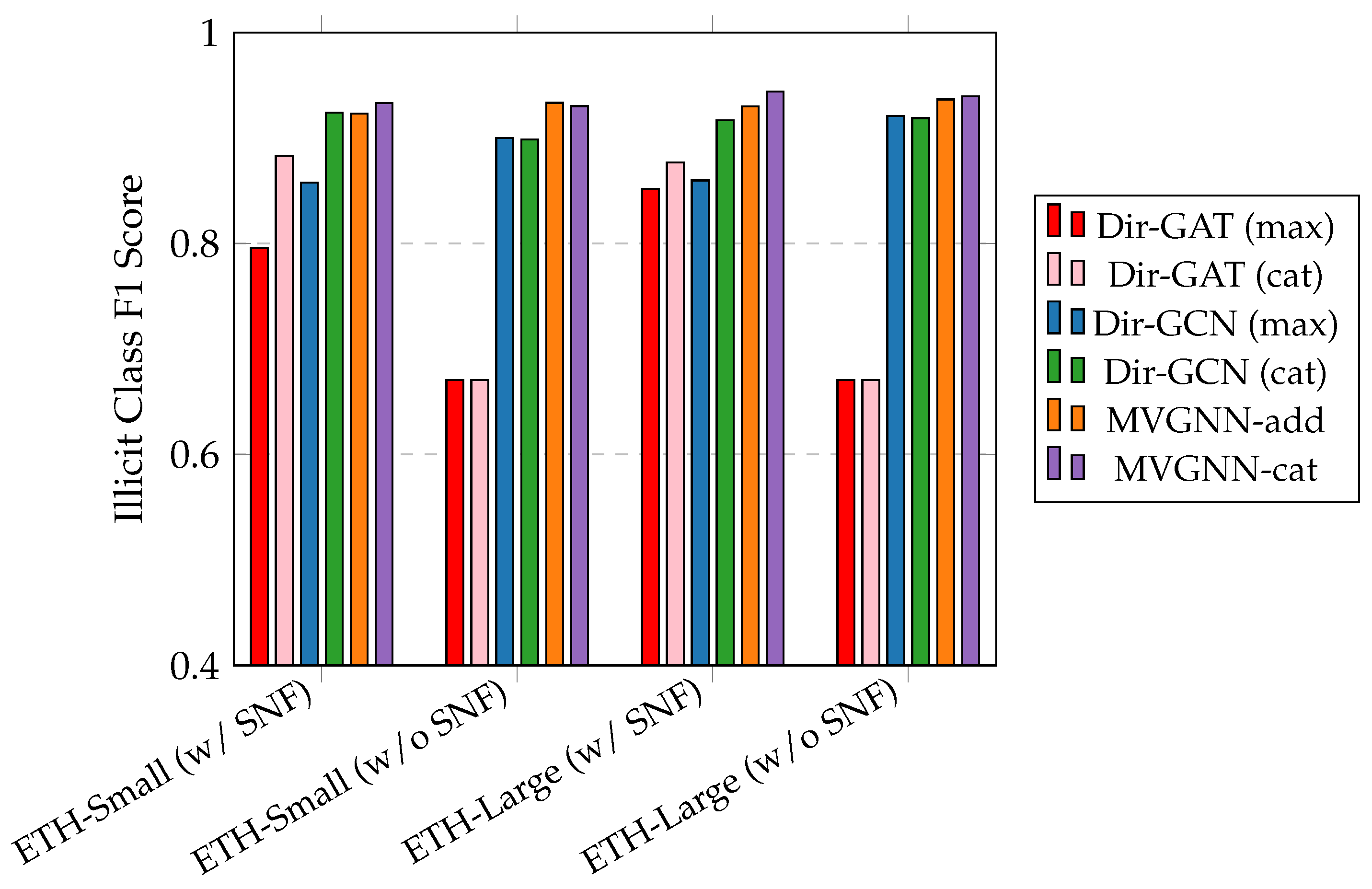
4.4.2. Effect of SNF

As shown in Table 2, regardless of the presence of different views, our LineMVGNN-cat model performs robustly when SNF (including node in-degrees and out-degrees) is masked in the ETH-Small and ETH-Large datasets. In addition, when LineMVGNN-cat is compared with LineMVGNN-add, message combination by concatenation is superior to the weighted sum method. Without SNF, the performance of LineMVGNN-add drops a little in various scenarios over Eth-Small and Eth-Large. Also, the performance of our LineMVGNN-cat model is less sensitive to the absence of SNF than LineMVGNN-add. This reflects the superiority of message combination by concatenation following a linear transformation over message combination by weighted sum.

4.4.3. Effect of Parameter Sharing

Our LineMVGNN variants extend from our MVGNN model, which is designed within the Dir-GNN framework due to its versatility. A key distinction between the MVGNN and Dir-GNN models lies in their parameter sharing approach. For Dir-GNN models, two independent sets of learnable parameters for ${\mathrm{M}}_{in}^{\left(l\right)}$ and ${\mathrm{M}}_{out}^{\left(l\right)}$ are used, theoretically enhancing expressiveness but doubling the number of parameters for each Dir-GNN layer. In contrast, our MVGNN models employ parameter sharing, creating a lighter yet effective model.

Our empirical experiments on real-world payment transaction datasets indicate that separating the two sets of learnable parameters may not always be necessary. As shown in Figure 4, the illicit class F1 scores of our MVGNN variants consistently outperform those of the Dir-GNN variants. On average, the F1 scores of our MVGNN-add surpasses those of the other competing methods by +7.01%, +21.48%, +6.22%, and +20.75% on the ETH-Small (w/ SNF), ETH-Small (w/o SNF), ETH-Large (w/ SNF), ETH-Large (w/o SNF), and FPT datasets, respectively. Meanwhile, our MVGNN-cat outperforms the others by +8.17%, +21.07%, +7.81%, and +21.12% on these five datasets, respectively.

4.4.4. Effect of Learning Rate

Learning rate can influence the training dynamics and final performance of deep learning models, such as LineMVGNN-add and LineMVGNN-cat. We conducted experiments with different learning rates chosen from $0.1,0.01,0.001$ while using default values for other hyperparameters on the ETH-Small (w/ or w/o SNF), ETH-Large (w/ or w/o SNF), and FPT datasets. The results are summarized in Figure 5, Figure 6 and Figure 7.

For the ETH-Small dataset (Figure 5) and the ETH-Large dataset (Figure 6), in general, the models achieve the highest F1 score for the illicit class at a learning rate of 0.01 regardless of the presence of SNF. A large learning rate of 0.1 leads to an unstable suboptimal performance, likely due to overshooting the optimal weights during gradient descent. Conversely, a small learning rate of 0.001 results in slower convergence and slightly lower performance in general. The models might have got trapped in local minima during training.

For the FPT dataset (Figure 7), the model performs best with a small learning rate of 0.001. This dataset is more complex, with more attributes and a larger number of nodes and edges. A smaller learning rate allows for more stable training, reducing the risk of overshooting the optimal solution, leading to better generalization. A large learning rate of 0.1 results in poor performance due to the instability of training, while a learning rate of 0.01 performs well but not as effectively as 0.001.

Comparing LineMVGNN-cat and LineMVGNN-add, although both variants exhibit similar behavior under the variation of learning rates, LineMVGNN-add is more robust to the variation of learning rate, especially when the transaction graph data is more complex. As shown in Figure 7 for the FPT dataset, although both variant models score over 0.99 for the illicit class F1, LineMVGNN-add’s performance degrades less noticeably than LineMVGNN-cat when the learning rate increases from 0.001 to 0.1. This reflects that LineMVGNN-cat, which combines messages from in- and out-neighbors via concatenation followed by a linear transformation, requires more careful tuning to ensure stable convergence. The linear transformation layer in LineMVGNN-cat introduces more learnable parameters, making the model more susceptible to oscillations or divergence if the learning rate is too high.

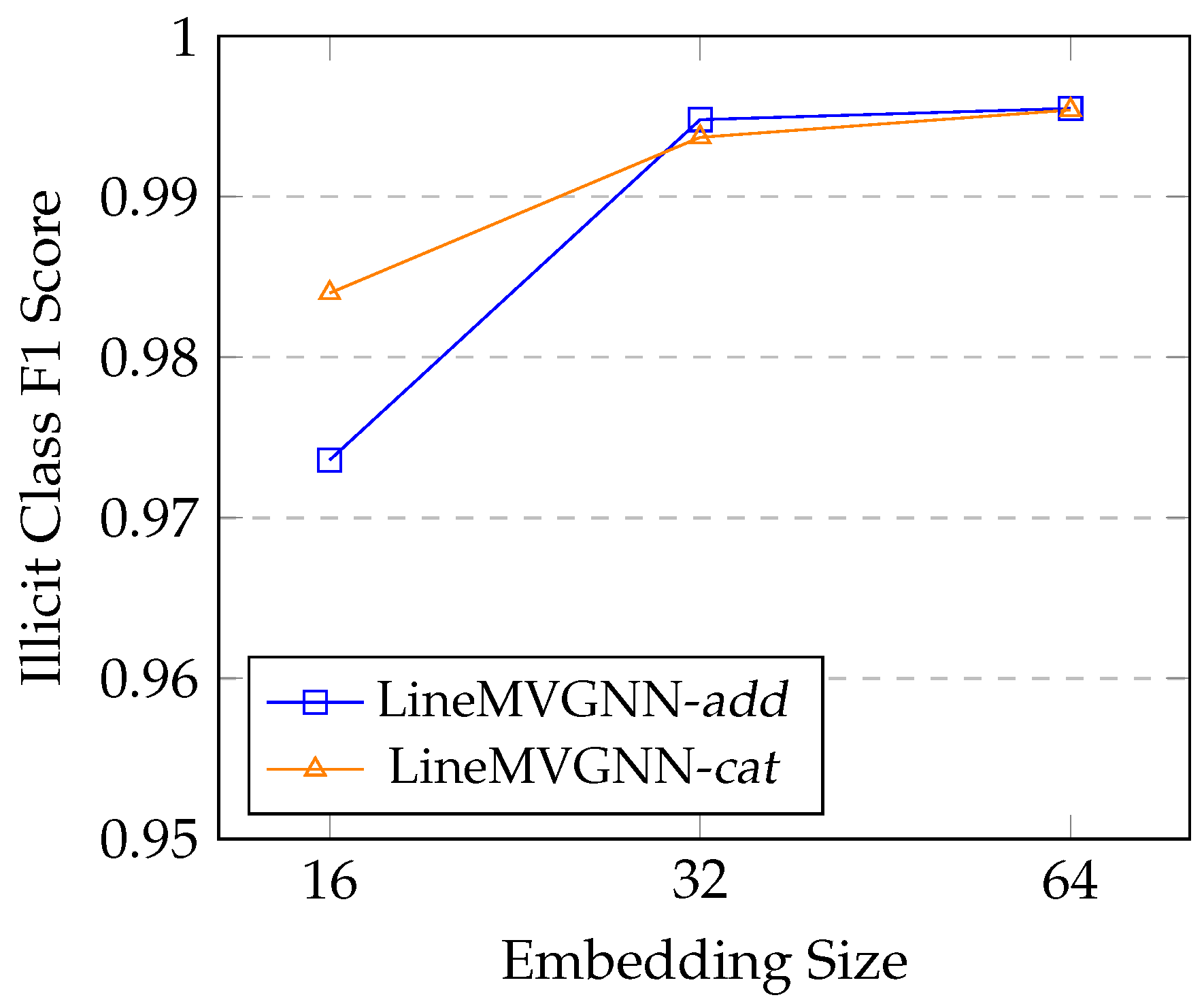
4.4.5. Effect of Embedding Size

The embedding size determines the dimensionality of the node and edge representations learned by the models. Generally, a larger embedding size can capture more complex patterns and nuances in the data. To explore the impact of embedding size on the performance of our LineMVGNN variants, we conduct experiments with different embedding sizes on the FPT dataset.

As shown in Figure 8, we vary embedding sizes of 16, 32, and 64. The models achieve the highest F1 score for the illicit class with an embedding size of 64. An embedding size of 32 results in a significant drop in the F1 score, likely due to insufficient capacity to capture the complex relationships in the transaction graph. On the other hand, doubling the embedding size from 32 to 64 provides little improvement: $+0.1711\%$ and $+0.0704\%$ for LineMVGNN-cat and LineMVGNN-add, respectively. The results suggest that an embedding size of 32 or 64 provides a good balance between model capacity and computational efficiency for the FPT dataset, while avoiding the pitfalls of overfitting and excessive computational cost associated with larger embedding sizes.

Comparing LineMVGNN-cat and LineMVGNN-add, LineMVGNN-cat, which leverages concatenation for message combination, is less sensitive to the increase in embedding size when the size doubles from 16. In contrast, LineMVGNN-add, which uses a weighted sum for message aggregation, is slightly less robustness. Its performance drops more noticeably with smaller embedding sizes. This suggests that the weighted sum mechanism may struggle to capture sufficient information with lower-dimensional representations. This difference highlights the advantage of LineMVGNN-cat’s concatenation-based approach, which provides greater flexibility in combining features and is less sensitive to embedding size variations.

Overall, both models benefit from an embedding size of 64, but LineMVGNN-cat demonstrates superior stability and performance across different embedding sizes, particularly in more complex datasets like FPT. We did not experiment on the ETH-Small and ETH-Large datasets due to the lack of attributes in the datasets. There are only three attributes in the datasets, which are transaction timestamps and amounts, and a label to indicate all fraud nodes. Given the limited feature set, the embedding size was set to match the dimensionality of the available attributes, ensuring that the model could effectively capture the sparse information present in the ETH datasets.

4.4.6. Qualitative Discussion

LineMVGNN improves over existing methods primarily through its ability to effectively propagate and leverage transaction-level information, which is crucial for AML detection. Unlike traditional GNNs that focus solely on node-level interactions, LineMVGNN introduces a line graph view that explicitly models edge (transaction) adjacencies. This allows the model to capture the flow of money between transactions, which is essential for identifying suspicious patterns such as temporary repositories of funds or cyclic transactions. By propagating edge features before updating node features, LineMVGNN ensures that transaction-level details are preserved and utilized in the learning process. Additionally, the two-way message passing mechanism in LineMVGNN (and in MVGNN), which considers both in- and out-neighbors, enhances the model’s ability to capture the directional flow of funds, further improving its detection capabilities. These features collectively enable LineMVGNN to outperform other competing methods, as demonstrated by its superior performance on the ETH-Small (w/ or w/o SNF), ETH-Large (w/ or w/o SNF), and FPT datasets.

5. Limitations and Future Work

5.1. Scalability

While the asymptotic computational complexity of our refined LineMVGNN model has the same asymptotic complexity $\mathcal{O}\left(L\right|\mathcal{E}\left|\right)$ as GCN [25], the refined LineMVGNN may have a higher practical runtime due to the additional overhead of edge propagation. Processing the entire graph in a single batch may not be feasible for extremely large graphs due to memory constraints. To alleviate this, graph sampling techniques can be leveraged, yielding smaller subgraphs for minibatch training.

5.2. Adversarial Robustness

In financial applications such as fraud detection, malicious actors may attempt to manipulate the graph to evade detection. Our current setup does not apply adversarial training for the model. In our future work, we can generate perturbed versions of the graphs during training and optimizing the model to perform well on both clean and perturbed data. On the other hand, before applying the model, graph purification can be integrated into the model, detecting and removing adversarial edges (transactions) or nodes (accounts). These techniques can enhance the model’s resilience to adversarial perturbations.

5.3. Regulatory Considerations

When deploying neural network models in highly regulated domains such as finance, the transparency and traceability of decisions are paramount. The proposed LineMVGNN model inherently provides explainability by explicitly modeling and propagating edge-level information (e.g., transactions) and aggregating it to the node level (e.g., accounts). This design allows the model to propagate and compare transactions (edge information) related to the same account (node). This highlights the contributions of individual edges (transactions) to the final node representations, making its decision-making process interpretable. For further improvement, explainable artificial intelligence (XAI) techniques can be integrated into the model, such as attention mechanisms and post hoc explainability methods.

6. Conclusions

Existing GNNs for digraphs face different challenges such as ignoring multi-dimensional edge features, the lack of model interpretability, and suboptimal model efficiency. To address these issues, we introduce a lighter-weight yet effective model, MVGNN, which shares parameters in the aggregation maps for payment and receipt transactions. This effectively and efficiently leverages the local original view and the local reversed view. Extended from MVGNN, we propose LineMVGNN which leverages line graph transformation for the enhanced propagation of transaction information. LineMVGNN surpasses SOTA methods in detecting money laundering activities and other financial frauds in real-world datasets.

References

1. Chen, Z.; Khoa, L.D.; Teoh, E.N.; Nazir, A.; Karuppiah, E.K.; Lam, K.S. Machine learning techniques for anti-money laundering (AML) solutions in suspicious transaction detection: A review. Knowl. Inf. Syst. 2018, 57, 245–285. [Google Scholar] [CrossRef]
2. Hilal, W.; Gadsden, S.A.; Yawney, J. Financial Fraud: A Review of Anomaly Detection Techniques and Recent Advances. Expert Syst. Appl. 2022, 193, 116429. [Google Scholar] [CrossRef]
3. Motie, S.; Raahemi, B. Financial fraud detection using graph neural networks: A systematic review. Expert Syst. Appl. 2024, 240, 122156. [Google Scholar] [CrossRef]
4. Koke, C.; Cremers, D. HoloNets: Spectral Convolutions do extend to Directed Graphs. In Proceedings of the Twelfth International Conference on Learning Representations, ICLR 2024, Vienna, Austria, 7–11 May 2024. [Google Scholar]
5. Fiorini, S.; Coniglio, S.; Ciavotta, M.; Messina, E. SigMaNet: One laplacian to rule them all. In Proceedings of the Thirty-Seventh AAAI Conference on Artificial Intelligence and Thirty-Fifth Conference on Innovative Applications of Artificial Intelligence and Thirteenth Symposium on Educational Advances in Artificial Intelligence, AAAI’23/IAAI’23/EAAI’23, Washington, DC, USA, 7–14 February 2023; AAAI Press: Washington, DC, USA, 2023. [Google Scholar] [CrossRef]
6. Zhang, X.; He, Y.; Brugnone, N.; Perlmutter, M.; Hirn, M.J. MagNet: A Neural Network for Directed Graphs. In Proceedings of the NeurIPS, Online, 6–14 December 2021; Ranzato, M., Beygelzimer, A., Dauphin, Y.N., Liang, P., Vaughan, J.W., Eds.; Curran Associates, Inc.: Red Hook, NY, USA, 2021; pp. 27003–27015. [Google Scholar]
7. Tong, Z.; Liang, Y.; Sun, C.; Li, X.; Rosenblum, D.S.; Lim, A. Digraph Inception Convolutional Networks. In Proceedings of the Advances in Neural Information Processing Systems 33: Annual Conference on Neural Information Processing Systems 2020, NeurIPS 2020, Virtual, 6–12 December 2020; Larochelle, H., Ranzato, M., Hadsell, R., Balcan, M., Lin, H., Eds.; Curran Associates, Inc.: Red Hook, NY, USA, 2020. [Google Scholar]
8. Tong, Z.; Liang, Y.; Sun, C.; Rosenblum, D.S.; Lim, A. Directed Graph Convolutional Network. arXiv 2020, arXiv:2004.13970. [Google Scholar]
9. Ma, Y.; Hao, J.; Yang, Y.; Li, H.; Jin, J.; Chen, G. Spectral-based Graph Convolutional Network for Directed Graphs. arXiv 2019, arXiv:1907.08990. [Google Scholar]
10. Monti, F.; Otness, K.; Bronstein, M.M. MotifNet: A motif-based Graph Convolutional Network for directed graphs. arXiv 2018, arXiv:1802.01572. [Google Scholar]
11. Rossi, E.; Charpentier, B.; Giovanni, F.D.; Frasca, F.; Günnemann, S.; Bronstein, M.M. Edge Directionality Improves Learning on Heterophilic Graphs. In Proceedings of the LoG, PMLR, Virtual, 27–30 November 2023; Villar, S., Chamberlain, B., Eds.; PMLR: London, UK, 2023; Volume 231, p. 25. [Google Scholar]
12. Thost, V.; Chen, J. Directed Acyclic Graph Neural Networks. In Proceedings of the 9th International Conference on Learning Representations, ICLR 2021, Virtual, Austria, 3–7 May 2021. [Google Scholar]
13. Li, Y.; Tarlow, D.; Brockschmidt, M.; Zemel, R.S. Gated Graph Sequence Neural Networks. In Proceedings of the 4th International Conference on Learning Representations, ICLR 2016, San Juan, PR, USA, 2–4 May 2016. [Google Scholar]
14. Gilmer, J.; Schoenholz, S.S.; Riley, P.F.; Vinyals, O.; Dahl, G.E. Neural Message Passing for Quantum Chemistry. In Proceedings of the 34th International Conference on Machine Learning, ICML 2017, Sydney, NSW, Australia, 6–11 August 2017; Precup, D., Teh, Y.W., Eds.; PMLR: London, UK, 2017; Volume 70, pp. 1263–1272. [Google Scholar]
15. Scarselli, F.; Gori, M.; Tsoi, A.C.; Hagenbuchner, M.; Monfardini, G. The Graph Neural Network Model. IEEE Trans. Neural Netw. 2009, 20, 61–80. [Google Scholar] [CrossRef] [PubMed]
16. Joint Financial Intelligence Unit. Screen the Account for Suspicious Indicators: Recognition of a Suspicious Activity Indicator or Indicators. 2024. Available online: https://www.jfiu.gov.hk/en/str_screen.html (accessed on 10 August 2024).
17. Bahmani, B.; Chowdhury, A.; Goel, A. Fast incremental and personalized PageRank. Proc. VLDB Endow. 2010, 4, 173–184. [Google Scholar] [CrossRef]
18. Velickovic, P.; Cucurull, G.; Casanova, A.; Romero, A.; Liò, P.; Bengio, Y. Graph Attention Networks. In Proceedings of the 6th International Conference on Learning Representations, ICLR 2018, Vancouver, BC, Canada, 30 April–3 May 2018. [Google Scholar]
19. Chen, Z.; Li, L.; Bruna, J. Supervised Community Detection with Line Graph Neural Networks. In Proceedings of the 7th International Conference on Learning Representations, ICLR 2019, New Orleans, LA, USA, 6–9 May 2019. [Google Scholar]
20. Liang, J.; Pu, C. Line Graph Neural Networks for Link Weight Prediction. arXiv 2023, arXiv:2309.15728. [Google Scholar]
21. Morshed, M.G.; Sultana, T.; Lee, Y.K. LeL-GNN: Learnable Edge Sampling and Line Based Graph Neural Network for Link Prediction. IEEE Access 2023, 11, 56083–56097. [Google Scholar] [CrossRef]
22. Zhang, H.; Xia, J.; Zhang, G.; Xu, M. Learning Graph Representations Through Learning and Propagating Edge Features. IEEE Trans. Neural Netw. Learn. Syst. 2024, 35, 8429–8440. [Google Scholar] [CrossRef] [PubMed]
23. Jiang, X.; Ji, P.; Li, S. CensNet: Convolution with Edge-Node Switching in Graph Neural Networks. In Proceedings of the IJCAI, Macao, 10–16 August 2019; Kraus, S., Ed.; AAAI Press: Washington, DC, USA, 2019; pp. 2656–2662. [Google Scholar]
24. Li, M.; Meng, L.; Ye, Z.; Xiao, Y.; Cao, S.; Zhao, H. Line graph contrastive learning for node classification. J. King Saud Univ. Comput. Inf. Sci. 2024, 36, 102011. [Google Scholar] [CrossRef]
25. Kipf, T.N.; Welling, M. Semi-Supervised Classification with Graph Convolutional Networks. In Proceedings of the 5th International Conference on Learning Representations, ICLR 2017, Toulon, France, 24–26 April 2017. [Google Scholar]
26. Hamilton, W.L.; Ying, Z.; Leskovec, J. Inductive Representation Learning on Large Graphs. In Proceedings of the NIPS, Long Beach, CA, USA, 4–9 December 2017; Guyon, I., von Luxburg, U., Bengio, S., Wallach, H.M., Fergus, R., Vishwanathan, S.V.N., Garnett, R., Eds.; Curran Associates Inc.: Red Hook, NY, USA, 2017; pp. 1024–1034. [Google Scholar]
27. Xu, K.; Hu, W.; Leskovec, J.; Jegelka, S. How Powerful are Graph Neural Networks? In Proceedings of the 7th International Conference on Learning Representations, ICLR 2019, New Orleans, LA, USA, 6–9 May 2019.
28. Gong, Z.; Wang, G.; Sun, Y.; Liu, Q.; Ning, Y.; Xiong, H.; Peng, J. Beyond Homophily: Robust Graph Anomaly Detection via Neural Sparsification. In Proceedings of the IJCAI, Macao, 19–25 August 2023; pp. 2104–2113. [Google Scholar]
29. Chien, E.; Peng, J.; Li, P.; Milenkovic, O. Adaptive Universal Generalized PageRank Graph Neural Network. In Proceedings of the 9th International Conference on Learning Representations, ICLR 2021, Virtual, Austria, 3–7 May 2021. [Google Scholar]
30. Cardoso, M.; Saleiro, P.; Bizarro, P. LaundroGraph: Self-Supervised Graph Representation Learning for Anti-Money Laundering. In Proceedings of the Third ACM International Conference on AI in Finance, ICAIF ’22, New York, NY, USA, 2–4 November 2022; pp. 130–138. [Google Scholar] [CrossRef]
31. Misra, I.; Shrivastava, A.; Gupta, A.; Hebert, M. Cross-Stitch Networks for Multi-task Learning. In Proceedings of the 2016 IEEE Conference on Computer Vision and Pattern Recognition, CVPR 2016, Las Vegas, NV, USA, 27–30 June 2016; IEEE Computer Society: Piscataway, NJ, USA, 2016; pp. 3994–4003. [Google Scholar] [CrossRef]
32. He, K.; Zhang, X.; Ren, S.; Sun, J. Deep Residual Learning for Image Recognition. In Proceedings of the 2016 IEEE Conference on Computer Vision and Pattern Recognition, CVPR 2016, Las Vegas, NV, USA, 27–30 June 2016; IEEE Computer Society: Piscataway, NJ, USA, 2016; pp. 770–778. [Google Scholar] [CrossRef]
33. Kanezashi, H.; Suzumura, T.; Liu, X.; Hirofuchi, T. Ethereum Fraud Detection with Heterogeneous Graph Neural Networks. arXiv 2022, arXiv:2203.12363. [Google Scholar]
34. Wu, J.; Yuan, Q.; Lin, D.; You, W.; Chen, W.; Chen, C.; Zheng, Z. Who Are the Phishers? Phishing Scam Detection on Ethereum via Network Embedding. IEEE Trans. Syst. Man Cybern. Syst. 2022, 52, 1156–1166. [Google Scholar] [CrossRef]
35. Elliott, A.; Cucuringu, M.; Luaces, M.M.; Reidy, P.; Reinert, G. Anomaly Detection in Networks with Application to Financial Transaction Networks. arXiv 2019, arXiv:1901.00402. [Google Scholar]
36. Corso, G.; Cavalleri, L.; Beaini, D.; Liò, P.; Velickovic, P. Principal Neighbourhood Aggregation for Graph Nets. In Proceedings of the Advances in Neural Information Processing Systems 33: Annual Conference on Neural Information Processing Systems 2020, NeurIPS 2020, Virtual, 6–12 December 2020; Larochelle, H., Ranzato, M., Hadsell, R., Balcan, M., Lin, H., Eds.; Curran Associates, Inc.: Red Hook, NY, USA, 2020. [Google Scholar]
37. Kamiński, K.; Ludwiczak, J.; Jasiński, M.; Bukala, A.; Madaj, R.; Szczepaniak, K.; Dunin-Horkawicz, S. Rossmann-toolbox: A deep learning-based protocol for the prediction and design of cofactor specificity in Rossmann fold proteins. Brief. Bioinform. 2021, 23, bbab371. [Google Scholar] [CrossRef] [PubMed]
38. Xu, K.; Li, C.; Tian, Y.; Sonobe, T.; Kawarabayashi, K.; Jegelka, S. Representation Learning on Graphs with Jumping Knowledge Networks. In Proceedings of the 35th International Conference on Machine Learning, ICML 2018, PMLR, Stockholm, Sweden, 10–15 July 2018; Dy, J.G., Krause, A., Eds.; PMLR: London, UK, 2018; Volume 80, pp. 5449–5458. [Google Scholar]
39. Hu, W.; Liu, B.; Gomes, J.; Zitnik, M.; Liang, P.; Pande, V.S.; Leskovec, J. Strategies for Pre-training Graph Neural Networks. In Proceedings of the 8th International Conference on Learning Representations, ICLR 2020, Addis Ababa, Ethiopia, 26–30 April 2020. [Google Scholar]
40. He, Y.; Zhang, X.; Huang, J.; Rozemberczki, B.; Cucuringu, M.; Reinert, G. PyTorch Geometric Signed Directed: A Software Package on Graph Neural Networks for Signed and Directed Graphs. In Proceedings of the Second Learning on Graphs Conference (LoG 2023), PMLR 231, Virtual, New Orleans, LA, USA, 27–30 November 2023. [Google Scholar]
41. Paszke, A.; Gross, S.; Massa, F.; Lerer, A.; Bradbury, J.; Chanan, G.; Killeen, T.; Lin, Z.; Gimelshein, N.; Antiga, L.; et al. PyTorch: An Imperative Style, High-Performance Deep Learning Library. In Proceedings of the Advances in Neural Information Processing Systems 32: Annual Conference on Neural Information Processing Systems 2019, NeurIPS 2019, Vancouver, BC, Canada, 8–14 December 2019; Wallach, H.M., Larochelle, H., Beygelzimer, A., d’Alché-Buc, F., Fox, E.B., Garnett, R., Eds.; Curran Associates, Inc.: Red Hook, NY, USA, 2019; pp. 8024–8035. [Google Scholar]
42. Wang, M.; Zheng, D.; Ye, Z.; Gan, Q.; Li, M.; Song, X.; Zhou, J.; Ma, C.; Yu, L.; Gai, Y.; et al. Deep Graph Library: A Graph-Centric, Highly-Performant Package for Graph Neural Networks. arXiv 2019, arXiv:1909.01315. [Google Scholar]
43. Fey, M.; Lenssen, J.E. Fast Graph Representation Learning with PyTorch Geometric. arXiv 2019, arXiv:1903.02428. [Google Scholar]
44. Kingma, D.P.; Ba, J. Adam: A Method for Stochastic Optimization. In Proceedings of the 3rd International Conference on Learning Representations, ICLR 2015, San Diego, CA, USA, 7–9 May 2015. [Google Scholar]
45. Loshchilov, I.; Hutter, F. SGDR: Stochastic Gradient Descent with Warm Restarts. In Proceedings of the 5th International Conference on Learning Representations, ICLR 2017, Toulon, France, 24–26 April 2017. [Google Scholar]
Figure 1. Hypothetical examples of benign and suspicious accounts in path patterns.
Ai 06 00069 g001
Figure 2. Visual illustration of two-way message passing in MVGNN.
Ai 06 00069 g002
Figure 3. Visual illustration of LineMVGNN.
Ai 06 00069 g003
Figure 4. Illicit class F1 score of Dir-GNN family and MVGNN family models across datasets.
Ai 06 00069 g004
Figure 5. Illicit class F1 against learning rate for ETH-Small (w/ or w/o SNF).
Ai 06 00069 g005
Figure 6. Illicit class F1 against learning rate for ETH-Large (w/ or w/o SNF).
Ai 06 00069 g006
Figure 7. Illicit class F1 against learning rate for FPT.
Ai 06 00069 g007
Figure 8. Illicit class F1 against embedding size for FPT dataset (w/ SNF).
Ai 06 00069 g008