Clinical Applicability of Machine Learning Models for Binary and Multi-Class Electrocardiogram Classification

Abstract

Background: This study investigates the application of machine learning models to classify electrocardiogram signals, addressing challenges such as class imbalances and inter-class overlap. In this study, “normal” and “abnormal” refer to electrocardiogram findings that either align with or deviate from a standard electrocardiogram, warranting further evaluation. “Borderline” indicates an electrocardiogram that requires additional assessment to distinguish benign variations from pathology. Methods: A hierarchical framework reformulated the multi-class problem into two binary classification tasks—distinguishing “Abnormal” from “Non-Abnormal” and “Normal” from “Non-Normal”—to enhance performance and interpretability. Convolutional neural networks, deep neural networks, and tree-based models, including Gradient Boosting Classifier and Random Forest, were trained and evaluated using standard metrics (accuracy, precision, recall, and F1 score) and learning curve convergence analysis. Results: Results showed that convolutional neural networks achieved the best balance between generalization and performance, effectively adapting to unseen data and variations without overfitting. They exhibit strong convergence and robust feature importance rankings, with ventricular rate, QRS duration, and P-R interval identified as key predictors. Tree-based models, despite their high performance metrics, demonstrated poor convergence, raising concerns about their reliability on unseen data. Deep neural networks achieved high sensitivity but suffered from overfitting, limiting their generalizability. Conclusions: The hierarchical binary classification approach demonstrated clinical relevance, enabling nuanced diagnostic insights. Furthermore, the study emphasizes the critical role of learning curve analysis in evaluating model reliability, beyond performance metrics alone. Future work should focus on optimizing model convergence and exploring hybrid approaches to improve clinical applicability in electrocardiogram signal classification.

1. Introduction

The analysis of electrocardiogram (ECG) signals has a long-standing history in medical science, dating back to the late 19th century when Willem Einthoven developed the first practical ECG machine [1,2,3], a contribution that earned him the Nobel Prize in 1924 [4]. Over the decades, advancements in technology have significantly improved the accuracy and accessibility of ECG devices, making them an indispensable tool in diagnosing cardiac abnormalities [5,6]. However, traditional diagnostic approaches often rely on manual interpretation [7,8], which can be time-consuming [9], prone to human error [10], and limited in handling large-scale datasets [11]. Recent developments in machine learning (ML) offer promising solutions to these challenges by automating ECG classification tasks with improved precision and scalability [12,13,14,15,16]. Despite their potential, ML models face critical issues such as overfitting [17], poor generalization to unseen data [18], and a lack of interpretability [19], particularly in clinical settings. Utilizing advanced ML architectures, such as convolutional neural networks and tree-based algorithms, in addition to addressing these challenges, could lead to the development of more reliable and clinically applicable tools for ECG signal classification. Recent systematic reviews and meta-analyses examining publications on this topic have highlighted the significant advancements in artificial intelligence (AI), ML, and deep learning (DL) applications for cardiovascular disease diagnoses and management using ECG. These reviews offer a detailed depiction of the current landscape across various cardiovascular ailments, emphasizing the growing importance of AI in ECG interpretation [20,21,22,23]. For example, a 2025 study explored research hotspots, trends, and future directions in the field of myocardial infarction and ML, highlighting the evolving landscape of ML applications in ECG analysis, particularly focusing on the challenges and future directions in this domain. The study emphasizes the need for continued research to address the current limitations and exploit the emerging opportunities in ML-based ECG classification, with neural networks playing a relevant role in early diagnosis, risk assessment, and rehabilitation therapy [24].

However, while many studies report strong classification metrics for ECG analysis, critical gaps remain in the validation protocols needed to ensure clinical applicability [25]. Claims of exceptional performance metrics often lack essential methodological rigor, e.g., many fail to demonstrate proper training dynamics through learning curves or validate classifier reliability across operational thresholds via metrics like receiver operating characteristic (ROC) curves. These omissions make it difficult to distinguish between genuine model generalizability versus dataset-specific overfitting, particularly given the inherent challenges of class imbalances and subtle diagnostic boundaries in ECG interpretation. The absence of convergence analyses in the reported training processes poses particular concerns. Learning curve comparisons between training and validation performance provide vital insights into whether models achieve stable, generalizable pattern recognition versus memorizing training artifacts [16]. As such, the reported accuracy rates in ECG classification prove clinically meaningless if model convergence analysis reveals divergence between training/validation trajectories, which is a hallmark of overfitting.

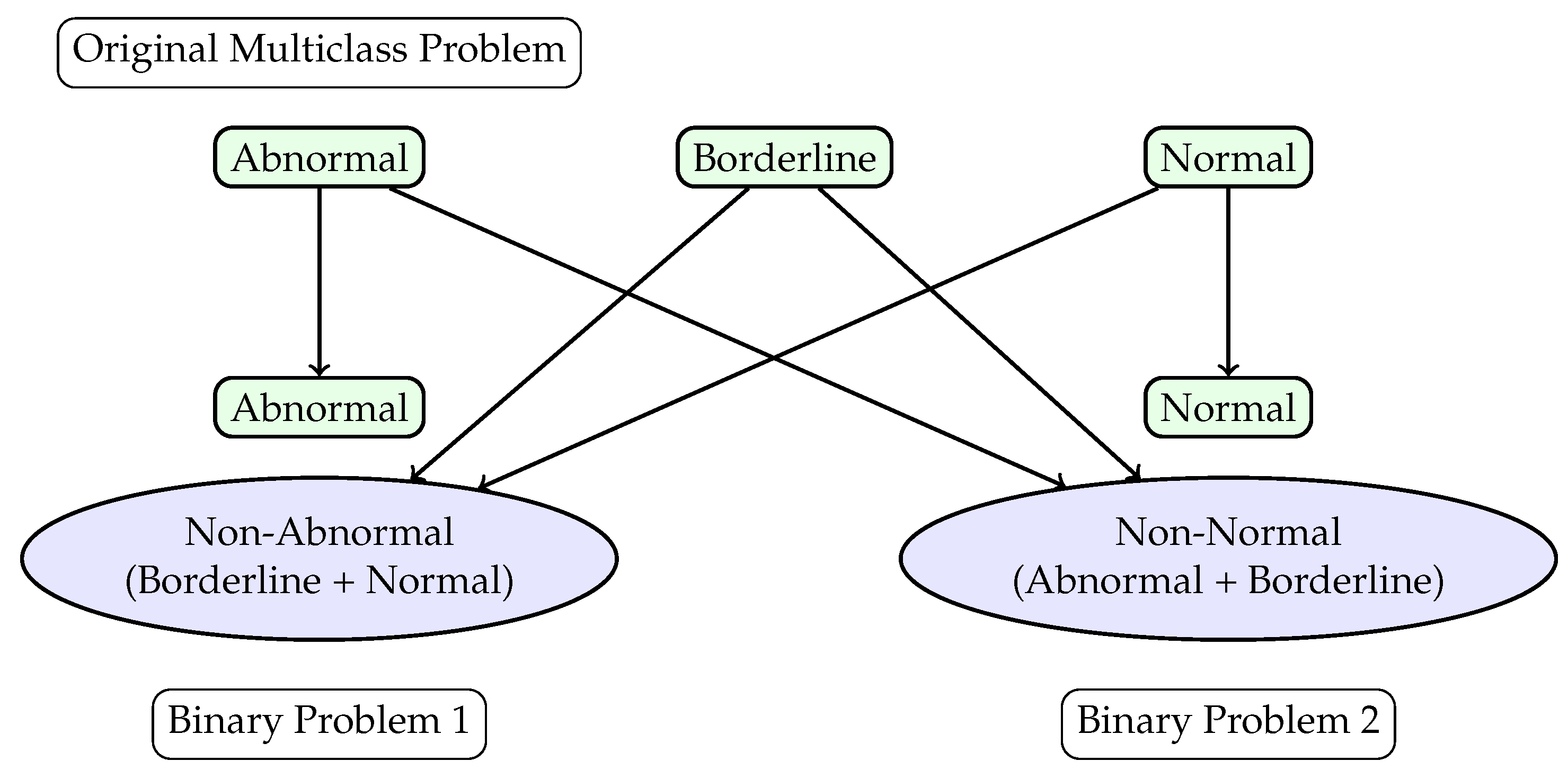
This study aims to evaluate the clinical applicability of various machine learning models for both binary and multi-class classification of ECG signals. The aim is to determine the most appropriate techniques and ML architecture for screening abnormal ECG studies while maintaining an appropriate level of generalizability and interpretability, i.e., issues that are common with current models [17,18,19]. To improve performance and interpretability, a hierarchical framework is utilized, which reformulates the multi-class classification problem into two binary classification tasks. All ECGs were labeled by clinicians as “normal”, “abnormal”, or “borderline”. “Normal” and “abnormal” refer to ECG findings that either conform to or deviate from a standard ECG, with abnormalities warranting further evaluation. “Borderline” indicates an ECG that requires additional assessment to differentiate benign variations from pathology. The first binary task differentiates between “Abnormal” and “Non-Abnormal” signals, where “Non-Abnormal” encompasses the “Borderline” and “Normal” classes. The second binary task distinguishes “Normal" from “Non-Normal” signals, where “Non-Normal” includes “Abnormal” and “Borderline” classes. This hierarchical approach seeks to mitigate the challenges posed by inter-class overlap and sn imbalanced data distribution.

The primary objective of this study is to identify the most effective machine learning model among convolutional neural networks (CNN), deep neural networks (DNN), and tree-based algorithms such as gradient boosting classifiers (GBC) and random forests (RF) in classifying ECG signals [26,27]. The evaluation considers accuracy, precision, recall, F1 score, and other standard performance metrics across both multi-class and binary classification tasks. Secondary objectives include analyzing the convergence behavior of the models through learning curve analysis, identifying key ECG features that influence classification, and investigating the trade-offs between sensitivity, specificity, and generalizability.

By addressing these objectives, the study aims to provide insights into the strengths and limitations of different machine learning approaches for ECG classification, contributing to the development of accurate and reliable tools for clinical decision support systems.

2. Materials and Methods

This section outlines the methodology employed to classify ECG signals using a hierarchical ML framework. The dataset used was collected by the authors. Patient data included sex, weight, history of diabetes, and history of smoking. From ECGs, the data extracted included Ventricular rate, atrial rate, PR-interval, QRS duration, QT interval, QTC calculation, P-axis, R-axis, and T-axis. These patients were classified into either “normal”, “borderline”, or “abnormal” based on their ECG data and patient data. The subsections detail the hierarchical classification approach (Section 2.1), which reformulates the original multi-class problem into two binary classification tasks to address challenges such as class imbalances and inter-class overlap. Section 2.2 describes the training procedures used for various ML models, including CNN, DNN, and tree-based algorithms, paying specific attention to data preprocessing, feature engineering, and model architectures. Section 2.2.1, Section 2.2.2 and Section 2.2.3 describe the specific implementation of CNNs, DNNs, and tree-based models, respectively, highlighting their configurations and optimization techniques. Section 2.3 discusses the evaluation metrics used to assess classification performance across the multi-class and binary tasks, including accuracy, precision, recall, F1 score, and specificity. Together, these sections provide an overview of the methodological framework.

2.1. Hierarchical Classification

The hierarchical classification framework used for ECG signal classification is illustrated in Figure 1. This framework structures the problem into multi-class and binary classification tasks to enhance model interpretability and performance. The original multi-class problem involves categorizing ECG signals into three distinct classes: Abnormal, Borderline, and Normal. The dataset was distributed into 2248 “Abnormal”, 1451 “Normal”, and 651 “Borderline” patients. To address inherent challenges such as inter-class overlap and imbalanced data distribution, the classification problem is reformulated into two binary tasks as follows. Binary Problem 1: The Borderline and Normal classes are combined into a single Non-Abnormal class, which is contrasted with the Abnormal class. In this problem, there were 2248 “Abnormal” and 2102 “Non-Abnormal” patients. Binary Problem 2: The Abnormal and Borderline classes are merged into a single Non-Normal class, which is contrasted with the Normal class. In this problem, there were 2899 “Non-Normal” and 1451 “Normal” patients.

This hierarchical approach allows for a focused evaluation of model performance across varying levels of complexity. ML models, including CNN and DNN architectures, GBC, RF, and Light Gradient Boosting Machine (LightGBM), were trained and tested on these classification tasks. The models were trained using preprocessed ECG signal data, with appropriate normalization and feature-scaling applied to ensure consistency across input data.

Performance metrics such as accuracy, sensitivity, specificity, precision, and F1 score were computed to evaluate the models’ ability to effectively classify ECG signals within both the multi-class and binary classification frameworks. This methodical breakdown facilitates a nuanced analysis of the model strengths and weaknesses, as detailed in subsequent sections.

2.2. Model Training for CNN, DNN, and Tree-Based Algorithms

The training of the CNN, DNN, and tree-based models using PyCaret was conducted as follows.

2.2.1. Convolutional Neural Network

The CNN model was constructed to classify ECG signals into binary categories: Normal and Abnormal. The data preprocessing included the removal of identifier columns, imputation of missing values using appropriate strategies for numerical and categorical variables, and encoding of categorical features using label encoding. Numerical features were scaled using standard normalization. To address class imbalances, the Synthetic Minority Oversampling Technique (SMOTE) was applied, generating a balanced dataset for training [28]. The input data for the CNN model were reshaped to a three-dimensional structure, $\mathbf{X}\in {\mathbb{R}}^{N\times F\times 1}$, suitable for one-dimensional convolutional layers, where N denotes the number of samples and F represents the number of features.

The CNN architecture consisted of two convolutional layers with ReLU activation functions and kernel sizes of 3, interleaved with max-pooling layers. Dropout layers with a rate of 0.3 were applied to mitigate overfitting. The final fully connected layers included a dense layer with 128 units, followed by the output layer with a sigmoid activation function for binary classification. The model’s loss function was binary cross-entropy:

$$\mathcal{L}=-{\displaystyle \frac{1}{N}}\sum _{i=1}^N\left[y_{i}log\left({\hat{y}}_i\right)+(1-y_i)log(1-{\hat{y}}_i)\right],$$

(1)

where $y_i$ and ${\hat{y}}_i$ represent the true and predicted labels for sample i, respectively. The Adam optimizer was employed to minimize the loss function. The model was trained over 50 epochs with a batch size of 32. Validation data were used to monitor performance and prevent overfitting.

The CNN architecture leverages hierarchical pattern recognition to disentangle overlapping ECG features. The initial convolutional layers detect localized temporal variations (e.g., QRS complex morphology or ST-segment deviations), while deeper layers integrate the contextual relationships between intervals (QT vs. RR durations) to resolve ambiguity. For example, the convolutional activations in layer 1 primarily correlate with atrial depolarization patterns (P-wave characteristics), and the layer 2 activations emphasize ventricular depolarization (QRS duration deviation). This hierarchical design mimics clinical ECG interpretation workflows, where clinicians first identify basic waveforms before assessing rhythm correlations.

Specifically, the CNN architecture employed 32 filters (kernel size = 3, ReLU activation) in the first convolutional layer, followed by max-pooling (pool size = 2) and batch normalization to regularize activations. The second convolutional layer utilized 64 filters (kernel size = 3) with identical pooling and normalization. A dropout rate of 0.5 was applied after the pooling layers to mitigate overfitting. For optimization, Adam (default settings: learning rate = 0.001, ${\beta }_1$ = 0.9, ${\beta }_2$ = 0.999) minimized binary cross-entropy loss. Input data were partitioned into stratified training (70%), validation (15%), and test (15%) sets using scikit-learn’s StratifiedKFold, preserving class distributions.

2.2.2. Deep Neural Network

The DNN model employed a fully connected architecture designed for binary ECG signal classification. The data preprocessing steps mirrored those used for CNN training, including imputation, encoding, and feature scaling. The input data were structured as a two-dimensional matrix $\mathbf{X}\in {\mathbb{R}}^{N\times F}$.

The DNN architecture included an input layer corresponding to the number of features, followed by two hidden layers with 128 and 64 neurons, respectively, each using ReLU activation. Dropout layers with a rate of 0.3 were included between the hidden layers to prevent overfitting. The output layer consisted of a single neuron with a sigmoid activation function for binary classification. The binary cross-entropy loss function (Equation (1)) and the Adam optimizer were used to train the model. Training was performed for 50 epochs with a batch size of 32. Model evaluation metrics included accuracy, precision, recall, F1 score, and misclassification.

Hence, the DNN comprised two hidden layers (128 and 64 units, ReLU activation) with batch normalization applied post-activation to stabilize training. Adam optimization maintained default hyperparameters (learning rate = 0.001, ${\beta }_1$ = 0.9, ${\beta }_2$ = 0.999) with early stopping (patience = 10 epochs, min delta = 0.001) to halt training if validation loss plateaued. Dropout (rate = 0.3) between dense layers reduced the co-adaptation of neurons.

2.2.3. PyCaret (Tree-Based Models)

Tree-based models were developed using the PyCaret library, which facilitated the comparison and selection of the most effective algorithms. Initially, 14 different ML models were compared, including RF, GBC, LightGBM, and other tree-based classifiers. PyCaret’s compare_models() function was utilized to evaluate these models based on the F1 score, allowing for an efficient ranking of their performance. Only the highest-performing models were selected for further hyperparameter tuning and optimization.

Across both binary classification tasks, multiple ML models (including LightGBM, GBC, and others) were trained and evaluated using PyCaret’s framework, with the best-performing model from each task selected for final comparison and analysis to ensure optimal performance.

The selected tree-based models underwent hyperparameter tuning using PyCaret’s tune_model() function to ensure optimal performance. A five-fold stratified cross-validation scheme was employed during training to enhance model robustness and generalizability [29]. For GBC, key hyperparameters included n_estimators=100 (default), learning_rate=0.1, and max_depth=3. The RF used n_estimators=100 and min_samples_split=2. Class weights were automatically adjusted during training to account for imbalanced distributions. Metrics such as accuracy, precision, recall, F1 score, and macro-average area under the ROC curve (AUC) were calculated to assess model performance. Feature importance visualizations provided additional interpretability by highlighting the most influential predictors.

The CNN and DNN models employed permutation-based feature importance to evaluate the relative contribution of each feature, while PyCaret’s tree-based models provided direct measures of feature importance. These analyses offered insights into the predictive capabilities of different input features, ensuring model interpretability and actionable results.

2.3. Performance Metrics

To evaluate the performance of the ML models used for ECG signal classification, several standard metrics were computed. These metrics included accuracy, precision, recall (sensitivity), specificity, F1 score, and misclassification rate. Each metric provides unique insights into the models’ performance, particularly in handling imbalanced datasets. The definitions of these metrics are as follows.

2.3.1. Accuracy

Accuracy measures the proportion of correctly classified instances out of the total number of instances. It is defined as

$$\mathrm{Accuracy}={\displaystyle \frac{TP+TN}{TP+TN+FP+FN}}$$

(2)

where $TP$ is the number of true positives, $TN$ is the number of true negatives, $FP$ is the number of false positives, and $FN$ is the number of false negatives.

2.3.2. Precision

Precision, also known as the positive predictive value, measures the proportion of correctly predicted positive instances out of all instances predicted as positive. It is given by the following equation:

$$\mathrm{Precision}={\displaystyle \frac{TP}{TP+FP}}$$

(3)

2.3.3. Recall (Sensitivity)

Recall, or sensitivity, measures the proportion of correctly predicted positive instances out of all actual positive instances. It is defined as

$$\mathrm{Recall}={\displaystyle \frac{TP}{TP+FN}}$$

(4)

2.3.4. Specificity

Specificity measures the proportion of correctly predicted negative instances out of all actual negative instances. It is calculated as

$$\mathrm{Specificity}={\displaystyle \frac{TN}{TN+FP}}$$

(5)

2.3.5. F1 Score

The F1 score is the harmonic mean of precision and recall, providing a single metric that balances the trade-off between these two measures. It is expressed as

$$F1=2·{\displaystyle \frac{\mathrm{Precision}·\mathrm{Recall}}{\mathrm{Precision}+\mathrm{Recall}}}$$

(6)

2.3.6. Misclassification Rate

The misclassification rate measures the proportion of incorrectly classified instances out of the total number of instances. It is the complement of accuracy and is defined as

$$\mathrm{Misclassification}\mathrm{Rate}=1-\mathrm{Accuracy}={\displaystyle \frac{FP+FN}{TP+TN+FP+FN}}$$

(7)

2.3.7. Class-Specific Metrics

For multi-class classification tasks, the metrics were computed for each class individually and then averaged using either the macro-average or weighted-average approach. Macro-Average: Metrics are computed independently for each class and then averaged, treating all classes equally. Weighted-Average: Metrics are computed independently for each class and then averaged, weighted by the number of instances in each class.

2.3.8. Evaluation Across Tasks

The performance metrics were computed for both the multi-class classification task and the two binary classification tasks described in Section 2.1. These metrics provide a comprehensive evaluation of the models’ ability to distinguish between the “Abnormal”, “Borderline”, and “Normal” classes, as well as the binary combinations of these classes.

2.3.9. Convergence Evaluation

The convergence behavior of each model was monitored using learning curves, which track performance using training and validation data over time. Proper convergence, indicated by synchronized and plateaued curves, is essential to ensure generalization and prevent overfitting or underfitting. Models were evaluated for their ability to reach stable performance during training, with attention paid to gaps between training and validation curves, which can reflect issues such as overfitting or poor learning. This analysis helps identify models that are both robust and reliable for unseen data.

2.3.10. Feature Importance Rankings

A feature importance analysis was conducted to determine the relative contribution of input features to model predictions. This provides insights into which features are most influential in the classification process and enhances interpretability. Neural network models, such as CNN and DNN, employed permutation-based techniques to assess feature relevance, while tree-based models inherently rank features based on their splits. These rankings are useful for understanding how models make decisions and ensuring alignment with clinical knowledge.

3. Results

The confusion matrices presented in Figure 2, Figure 3 and Figure 4 provide a comparative evaluation of the different ML models used for classifying ECG signals. These matrices, normalized for consistency, allow for a detailed analysis of the classification performance across various tasks and models. The results highlight the strengths and weaknesses of CNN, DNN, GBC, RF, and LightGBM models in both multi-class and binary classification scenarios. In Figure 2, the performance of CNN, DNN, and LightGBM models is compared for a multi-class classification task. The CNN model, shown in Figure 2a, demonstrates moderate performance, with its highest diagonal value reaching 56.94%, indicating the best classification accuracy for one of the classes. However, the off-diagonal values, such as 30.04% and 28.13%, reveal significant misclassification between certain classes, suggesting challenges in distinguishing between similar ECG signal patterns. The DNN model, depicted in Figure 2b, shows a slight improvement, with a maximum diagonal value of 59.72%. Despite this, the off-diagonal values remain high (e.g., 26.01% and 29.69%), indicating persistent inter-class confusion. The LightGBM model, shown in Figure 2c, achieves the highest diagonal value of 69.96%, reflecting superior accuracy for certain classes. However, the off-diagonal values, such as 28.25% and 42.19%, suggest that this model may overfit or exhibit sensitivity to specific features, leading to poor performance in other classification tasks.

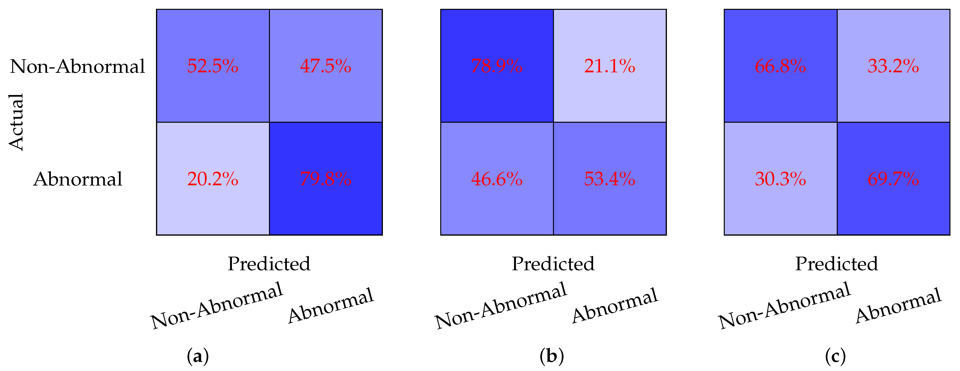
Figure 3 evaluates the model performance on a binary classification task where the Borderline and Normal classes are combined into a single Non-Abnormal class. The CNN model, shown in Figure 3a, achieves a sensitivity of 52.5% and a specificity of 79.8%. While the model performs well in identifying Non-Abnormal cases, its relatively low sensitivity indicates difficulty in detecting Abnormal cases. The DNN model, depicted in Figure 3b, demonstrates a significant improvement in sensitivity, reaching 78.9%, but its specificity drops to 53.4%. This suggests that the DNN model is better at identifying Abnormal cases but struggles with false positives in the Non-Abnormal class. The GBC model, shown in Figure 3c, achieves a more balanced performance, with a sensitivity of 66.8% and a specificity of 69.7%. This balance indicates that the GBC model provides consistent classification across both classes, making it a strong candidate for this binary classification task.

In Figure 4, the models are evaluated on a binary classification task where the Abnormal and Borderline classes are combined into a single Non-Normal class. The CNN model, shown in Figure 4a, achieves a sensitivity of 61.7% and a specificity of 66.0%. While the performance is relatively balanced, the low sensitivity indicates that the model struggles to detect Non-Normal cases effectively. The DNN model, depicted in Figure 4b, demonstrates a significant improvement in specificity, reaching 83.3%, but this comes at the cost of sensitivity, which drops to 33.5%. This suggests that the DNN model is highly conservative in classifying cases as Non-Normal, leading to a high rate of false negatives. The RF model, shown in Figure 4c, achieves a sensitivity of 82.58% and a specificity of 54.17%.

Overall, the results across Figure 2, Figure 3 and Figure 4 reveal several trends. LightGBM achieves the highest accuracy for multi-class classification, as shown in Figure 2c, while GBC and RF provide the most balanced performance for binary classification tasks, as seen in Figure 3c and Figure 4c. DNN models tend to favor either sensitivity or specificity depending on the task, while tree-based models such as GBC and RF offer more consistent performance. Multi-class classification, as shown in Figure 2, poses greater challenges for all models, as evidenced by the higher off-diagonal values compared to the binary classification tasks in Figure 3 and Figure 4. These findings underscore the importance of selecting the appropriate model based on the specific classification task and the desired balance between sensitivity and specificity.

The performance metrics for the classification of ECG signals are summarized in

Table 1. Overall accuracies (all correct/all).

	Abnormal/ Borderline/Normal	Abnormal/ Non-Abnormal	Non-Normal/ Normal
CNN	54.2%	65.7%	63.1%
DNN	59.7%	66.7%	50.1%
LGBM	59.9%	–	–
GBC	–	68.2%	–
RF	–	–	71.2%

,

Table 2. Overall misclassification rates (all incorrect/all).

	Abnormal/ Borderline/Normal	Abnormal/ Non-Abnormal	Non-Normal/ Normal
CNN	48.3%	34.3%	36.9%
DNN	43.2%	33.4%	49.9%
LGBM	40.1%	–	–
GBC	–	31.8%	–
RF	–	–	28.8%

,

Table 3. Overall sensitivities, aka recalls (true positives/all actual positives).

	Abnormal/ Borderline/Normal	Abnormal/ Non-Abnormal	Non-Normal/ Normal
CNN	70.5%	79.8%	78.3%
DNN	77.3%	53.4%	80.0%
LGBM	68.4%	–	–
GBC	–	70.3%	–
RF	–	–	78.2%

,

Table 4. Overall specificities (true negatives/all actual negatives).

	Abnormal/ Borderline/Normal	Abnormal/ Non-Abnormal	Non-Normal/Normal
CNN	60.8%	61.0%	46.3%
DNN	65.3%	70.3%	38.6%
LGBM	67.0%	–	–
GBC	–	66.2%	–
RF	–	–	60.9%

and

Table 5. Overall precisions (true positives/predicted positives).

	Abnormal/ Borderline/Normal	Abnormal/ Non-Abnormal	Non-Normal/ Normal
CNN	54.7%	73.6%	78.3%
DNN	59.6%	64.5%	80.0%
LGBM	69.9%	–	–
GBC	–	70.3%	–
RF	–	–	82.6%

. These tables provide an overview of the models’ accuracies, misclassification rates, sensitivities, specificities, and precisions across different classification tasks. The results highlight the strengths and weaknesses of the CNN, DNN, LightGBM, GBC, and RF models in handling various combinations of ECG signal classes.

Table 1 presents the overall accuracies for each model across the classification tasks. The CNN model achieves an accuracy of 54.2% for a multi-class task involving the Abnormal, Borderline, and Normal classes, which improves to 65.7% when the Borderline and Normal classes are combined into Non-Abnormal. For the binary classification task that combines Abnormal and Borderline into Non-Normal, the CNN achieves an accuracy of 63.1%. The DNN model performs slightly better in the multi-class task, with an accuracy of 59.7%, and achieves 66.7% for the Non-Abnormal classification. However, its accuracy drops to 50.1% for the Non-Normal classification. LightGBM achieves the highest accuracy for the multi-class task at 59.9%, while GBC achieves an accuracy of 68.2% for the Non-Abnormal classification. The RF model outperforms all others in the Non-Normal classification, achieving an accuracy of 71.2%.

The misclassification rates, presented in Table 2, offer valuable insights into the performance of the models. The CNN model has a misclassification rate of 48.3% for the multi-class task, which improves to 34.3% for the Non-Abnormal classification and 36.9% for the Non-Normal classification. In comparison, the DNN model exhibits a lower misclassification rate of 43.2% for the multi-class task and 33.4% for the Non-Abnormal classification; however, it has a higher misclassification rate of 49.9% for the Non-Normal classification. LightGBM achieves the lowest misclassification rate for the multi-class task, at 40.1%, while GBC records the lowest rate for the Non-Abnormal classification, at 31.8%. The RF model demonstrates the best performance for the Non-Normal classification, achieving a misclassification rate of 28.8%.

Table 3 provides an overview of the sensitivities (recalls) of the models, which assess their ability to accurately identify positive cases. The CNN model records a sensitivity of 70.5% for the multi-class task, which rises to 79.8% for Non-Abnormal classification and 78.3% for Non-Normal classification. The DNN model achieves the highest sensitivity for the multi-class task at 77.3%, but its performance drops significantly to 53.4% for Non-Abnormal classification, while it achieves 80.0% for Non-Normal classification. LightGBM shows a sensitivity of 68.4% for the multi-class task, and the GBC model achieves the highest sensitivity in Non-Abnormal classification at 70.3%. Additionally, the RF model reaches a sensitivity of 78.2% for Non-Normal classification.

Table 4 presents the specificities of the models, which indicate their ability to accurately identify negative cases. The CNN model reports a specificity of 60.8% for the multi-class task, 61.0% for Non-Abnormal classification, and 46.3% for Non-Normal classification. The DNN model shows a slightly better performance, with specificities of 65.3% for the multi-class task and 70.3% for Non-Abnormal classification, but its specificity significantly decreases to 38.6% for Non-Normal classification. LightGBM achieves the highest specificity for the multi-class task, at 67.0%, while the GBC model reaches the highest specificity for Non-Abnormal classification, at 66.2%. Lastly, the RF model records a specificity of 60.9% for Non-Normal classification.

Finally, Table 5 displays the overall precisions (positive predictive values) of the models, which indicate the proportion of predicted positive cases that are accurate. The CNN model achieves a precision of 54.7% for the multi-class task, improving to 73.6% for Non-Abnormal classification and 78.3% for Non-Normal classification. The DNN model records a precision of 59.6% for the multi-class task, 64.5% for Non-Abnormal classification, and 80.0% for Non-Normal classification. LightGBM achieves the highest precision for the multi-class task at 69.9%, while the GBC model reaches the highest precision for Non-Abnormal classification at 70.3%. Additionally, the RF model achieves a precision of 82.6% for Non-Normal classification.

The Table 1, Table 2, Table 3, Table 4 and Table 5 provide a detailed comparison of the models’ performance across different metrics and classification tasks. LightGBM demonstrates strong performance in the multi-class task, while GBC and RF models excel in the binary classification tasks. The CNN and DNN models show a balanced performance across metrics, with DNN achieving higher sensitivities and CNN achieving higher specificities in certain tasks. These results highlight the trade-offs between sensitivity, specificity, and precision, emphasizing the importance of selecting the appropriate model based on the specific requirements of the classification task.

Evaluating per-class metrics and then averaging them is essential, especially when working with imbalanced datasets, as relying solely on overall accuracy can be misleading. Overall accuracy provides a general sense of performance but often masks the model’s struggles with underrepresented classes. For instance, although LightGBM achieves the highest accuracy for the multi-class task (Table 1), a closer examination of the corresponding confusion matrix (Figure 4) and per-class metrics (

Table 6. Per-class metrics for the 3-class classification problem.

Model	Class	Precision	Recall	F1
CNN	Abnormal	0.705	0.547	0.615
	Borderline	0.209	0.297	0.245
	Normal	0.491	0.569	0.527
	Average	0.468	0.471	0.462
DNN	Abnormal	0.774	0.596	0.673
	Borderline	0.271	0.406	0.325
	Normal	0.528	0.597	0.560
	Average	0.524	0.533	0.519
LGBM	Abnormal	0.684	0.700	0.692
	Borderline	0.526	0.694	0.599
	Normal	0.154	0.031	0.052
	Average	0.455	0.475	0.448

) reveals that the model performs well on certain classes but struggles significantly with others, such as the “Normal” class, highlighting its inability to generalize effectively across all classes.

Hence, by examining per-class precision, recall, and F1 scores, it becomes clear which classes the model predicts well and which it struggles with. In the context of ECG signal classification, the importance of per-class metrics becomes even more evident. For example, in a three-class classification task, all models faced challenges with the “Borderline” class. This difficulty likely stems from the class’s overlap with other categories or its insufficient representation in the dataset. Among the evaluated models, the DNN model demonstrated the most balanced performance across all classes, achieving the highest average F1 score (Table 6). In contrast, the LightGBM model performed well on the “Abnormal” and “Borderline” classes but struggled significantly with the “Normal” class, suggesting potential overfitting. Meanwhile, the CNN showed moderate performance but lagged behind the DNN model in all metrics, indicating room for further optimization.

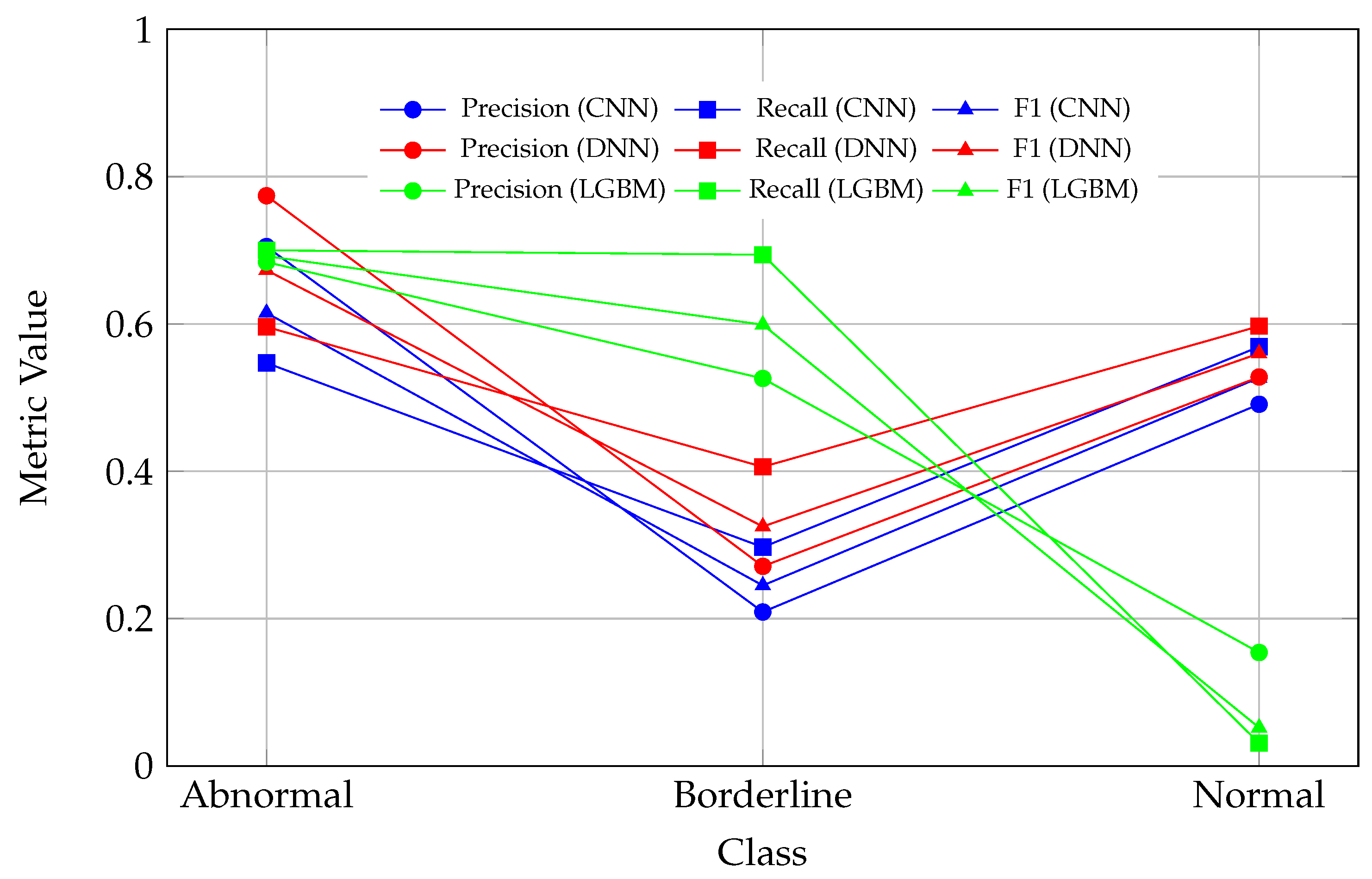
The observed drop in all metric values (precision, recall, and F1) for the Normal class in the LGBM model, as seen in Figure 5, indicates a significant challenge in correctly classifying instances of this class. This decline may reflect an imbalance in the dataset, where the Normal class is underrepresented, leading to insufficient learning during model training. Additionally, the features of the Normal class may overlap with those of other classes, such as Abnormal or Borderline, making it difficult for the models to distinguish between them. The LGBM model, in particular, appears to exhibit a bias toward other classes, potentially due to the distribution of the training data or the model’s inherent characteristics. Furthermore, the drop in performance could be attributed to noise or inconsistencies in the data associated with the Normal class, which may hinder the model’s ability to generalize effectively. The decline in metrics suggests that the model is producing a higher number of false positives or false negatives for this class, directly impacting the calculated precision, recall, and F1 scores.

The performance of the ML models in binary classification tasks was evaluated using per-class metrics, including precision, recall, and F1 scores. Two binary classification tasks were considered: (1) combining the “Borderline” and “Normal” classes into a single “Non-Abnormal” class, and (2) combining the “Abnormal” and “Borderline” classes into a single “Non-Normal” class. The results, presented in

Table 7. Per-class metrics for the two-class classification problem, when the ‘Borderline’ and ‘Normal’ classifications are combined into classification ‘Non-Abnormal’.

Model	Class	Precision	Recall	F1
CNN	Abnormal	0.736	0.525	0.613
	Non-Abnormal	0.610	0.798	0.692
	Average	0.673	0.662	0.653
DNN	Abnormal	0.645	0.789	0.710
	Non-Abnormal	0.703	0.534	0.608
	Average	0.674	0.662	0.659
GBC	Abnormal	0.703	0.668	0.685
	Non-Abnormal	0.662	0.697	0.679
	Average	0.683	0.683	0.682

and

Table 8. Per-class metrics for the two-class classification problem, when the ‘Abnormal’ and ‘Borderline’ classifications are combined into the classification ‘Non-Normal’.

Model	Class	Precision	Recall	F1
CNN	Normal	0.617	0.783	0.690
	Non-Normal	0.660	0.463	0.545
	Average	0.639	0.623	0.618
DNN	Normal	0.335	0.800	0.472
	Non-Normal	0.833	0.386	0.526
	Average	0.584	0.593	0.499
RF	Normal	0.826	0.782	0.804
	Non-Normal	0.542	0.609	0.573
	Average	0.684	0.696	0.689

, provide insights into the strengths and weaknesses of the CNN, DNN, GBC, and RF models in handling these tasks.

In the first binary classification task, where the “Borderline” and “Normal” classes were merged into the “Non-Abnormal” class (Table 7), the GBC model demonstrated the most balanced performance across all metrics. The GBC model achieved an average precision, recall, and F1 score of 0.683, outperforming both the CNN and DNN models in terms of consistency. The CNN model achieved an average precision of 0.673, recall of 0.662, and F1 score of 0.653, indicating moderate performance. However, the CNN model exhibited a stronger ability to identify “Non-Abnormal” cases, with a recall of 0.798 and an F1 score of 0.692, compared to its performance on the “Abnormal” class, where the recall was lower at 0.525 and the F1 score was 0.613. This suggests that the CNN model is more effective at identifying “Non-Abnormal” cases but struggles with sensitivity for the “Abnormal” class. The DNN model achieved slightly higher average metrics compared to the CNN model, with an average precision of 0.674, recall of 0.662, and F1 score of 0.659. The DNN model performed better on the “Abnormal” class, achieving a recall of 0.789 and an F1 score of 0.710, but its performance on the “Non-Abnormal” class was weaker, with a recall of 0.534 and an F1 score of 0.608. This indicates that the DNN model prioritizes sensitivity for the “Abnormal” class, potentially at the expense of false positives in the “Non-Abnormal” class. Overall, the GBC model provided the most consistent performance across both classes, making it a strong candidate for this binary classification task. The CNN and DNN models exhibited class-specific strengths, with CNN favoring the “Non-Abnormal” class and DNN favoring the “Abnormal” class.

In the second binary classification task, where the “Abnormal” and “Borderline” classes were combined into the “Non-Normal” class (Table 8), the RF model exhibited the most balanced performance. It achieved an average precision of 0.684, a recall of 0.696, and an F1 score of 0.689, demonstrating consistent metrics for both the “Normal” and “Non-Normal” classes. Specifically, the RF model attained an F1 score of 0.804 for the “Normal” class and 0.573 for the “Non-Normal” class, indicating its ability to maintain balanced performance across both categories. The CNN model recorded an average precision of 0.639, a recall of 0.623, and an F1 score of 0.618. It performed better on the “Normal” class, achieving a recall of 0.783 and an F1 score of 0.690, compared to the “Non-Normal” class, where the recall was lower at 0.463 and the F1 score was 0.545. This suggests that the CNN model is more effective at identifying “Normal” cases but struggles with sensitivity for the “Non-Normal” class, potentially leading to missed detections of abnormal signals. The DNN model demonstrated the weakest overall performance in this task, with an average precision of 0.584, a recall of 0.593, and an F1 score of 0.499. While it achieved a high recall of 0.800 for the “Normal” class, this came at the expense of low precision (0.335) and a modest F1 score of 0.472. For the “Non-Normal” class, the DNN model recorded a precision of 0.833 but a low recall of 0.386, resulting in an F1 score of 0.526. These results indicate that the DNN model is highly conservative in predicting “Non-Normal” cases, leading to a high rate of false negatives for this class.

Figure 6 and Figure 7 offer a comparative analysis of ML model performances for binary ECG classification tasks, specifically focusing on the relationships between precision, recall, and F1 scores. These figures are useful for determining the clinical applicability of different models in identifying and categorizing abnormal and borderline ECG signal patterns.

Figure 6 evaluates the performance of CNN, DNN models, and GBC in distinguishing between “Abnormal” and “Non-Abnormal” ECG signals. The CNN model displays a moderate classification performance, achieving higher recall and F1 scores for the “Non-Abnormal” class (recall: 79.8%; F1 score: 69.2%) compared to the “Abnormal” class (recall: 52.5%; F1 score: 61.3%). This suggests that while the CNN model is effective in ruling out abnormality, it struggles with sensitivity in detecting abnormal cases, which may lead to underdiagnosis. Conversely, the DNN model demonstrates a notable improvement in sensitivity for the “Abnormal” class (recall: 78.9%; F1 score: 71.0%) but a trade-off in specificity and performance for the “Non-Abnormal” class (recall: 53.4%; F1 score: 60.8%), indicating its focus on minimizing missed abnormalities at the expense of false positives. The GBC model emerges as the most balanced, with precision, recall, and F1 scores consistently around 68% for both classes, making it a reliable candidate for generalized clinical use where both sensitivity and specificity are required.

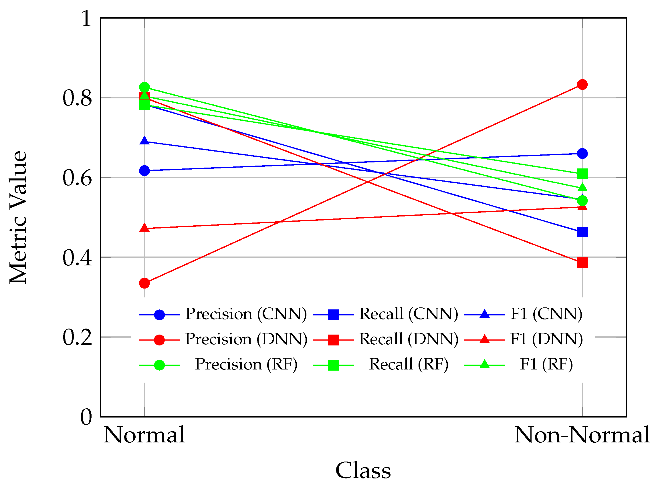
Figure 7 investigates the ability of CNN, DNN, and random forest (RF) models to distinguish between “Normal” and “Non-Normal” ECG signals (a combination of “Abnormal” and “Borderline” classes). The CNN model performs well in identifying “Normal” cases (recall: 78.3%; F1 score: 69.0%) but demonstrates weaker sensitivity for “Non-Normal” cases (recall: 46.3%; F1 score: 54.5%), underscoring its limited utility in detecting borderline or abnormal signals. The DNN model, while achieving high specificity for “Non-Normal” cases (precision: 83.3%), produces a low recall (38.6%), leading to an imbalanced F1 score (52.6%). This indicates that the DNN model is overly conservative when classifying “Non-Normal” cases, resulting in a high rate of missed abnormalities. The RF model, by contrast, demonstrates the most balanced performance, with an F1 score of 80.4% for “Normal” cases and 57.3% for “Non-Normal” cases, highlighting its clinical reliability in distinguishing between normal and non-normal ECG signals.

From a clinical perspective, these figures emphasize the trade-offs each model makes between sensitivity and specificity. The DNN model prioritizes sensitivity for abnormal cases, aligning with clinical scenarios where detecting every possible abnormality is critical to avoid missed diagnoses. However, its tendency to generate false positives could lead to unnecessary follow-ups or interventions. The CNN model, on the other hand, provides better specificity, making it more suitable for confirming normality or ruling out abnormality in less critical scenarios. The GBC and RF models offer a balanced performance across tasks, making them ideal for general clinical applications where both sensitivity and specificity are essential. Notably, all models face challenges in distinguishing borderline cases, reflecting the inherent complexity and overlap of this class with normal and abnormal patterns.

3.1. Convergence—Learning Curves

Convergence in ML refers to the stabilization of learning curves as the model’s training progresses, where both the training and validation performance reach a plateau. A healthy convergence is observed when the training and validation curves rise together, reaching an asymptotic limit, with the validation performance slightly lower than the training performance. This behavior indicates that the model is learning effectively from the training data while maintaining its ability to generalize to unseen data.

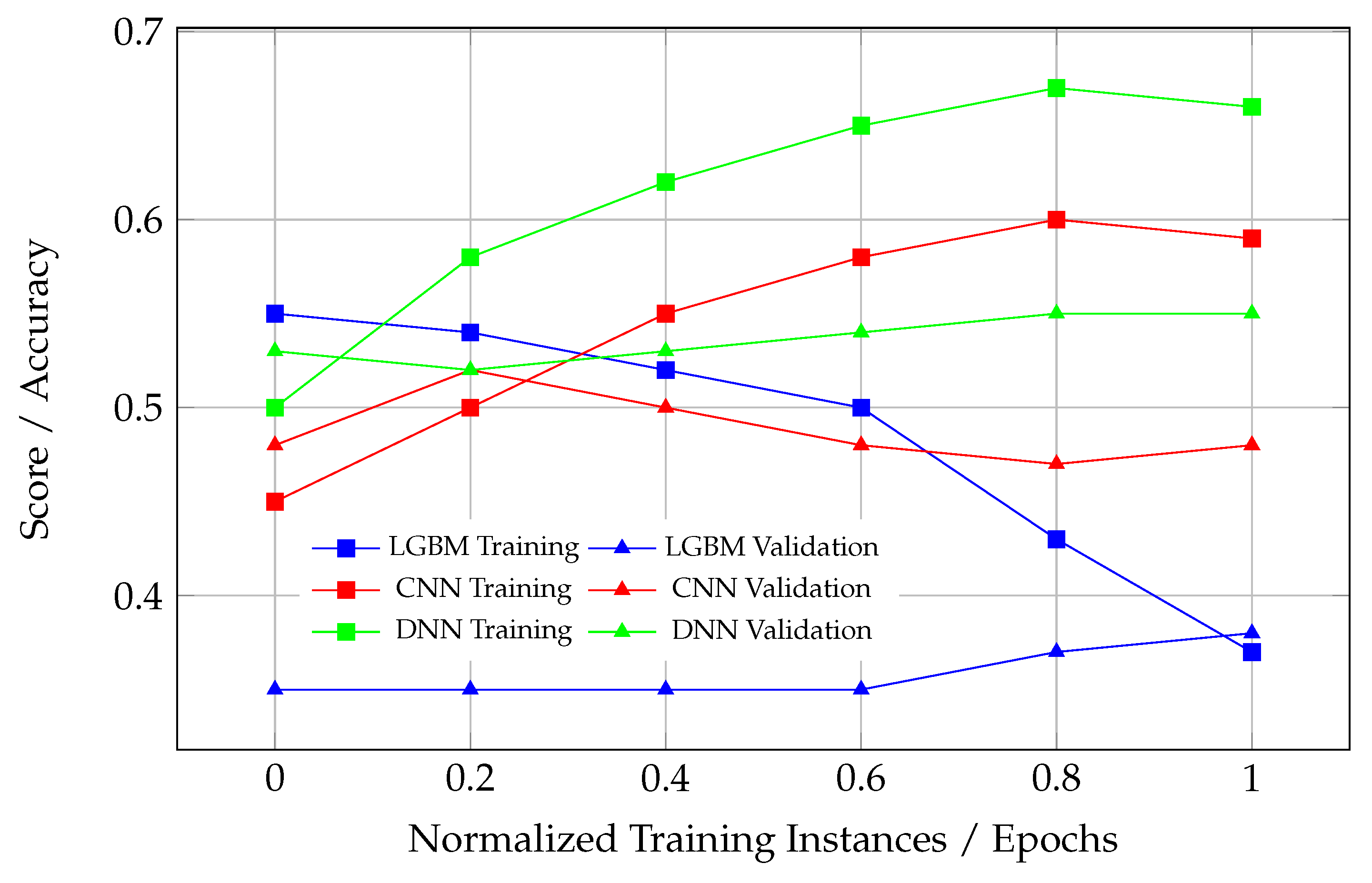
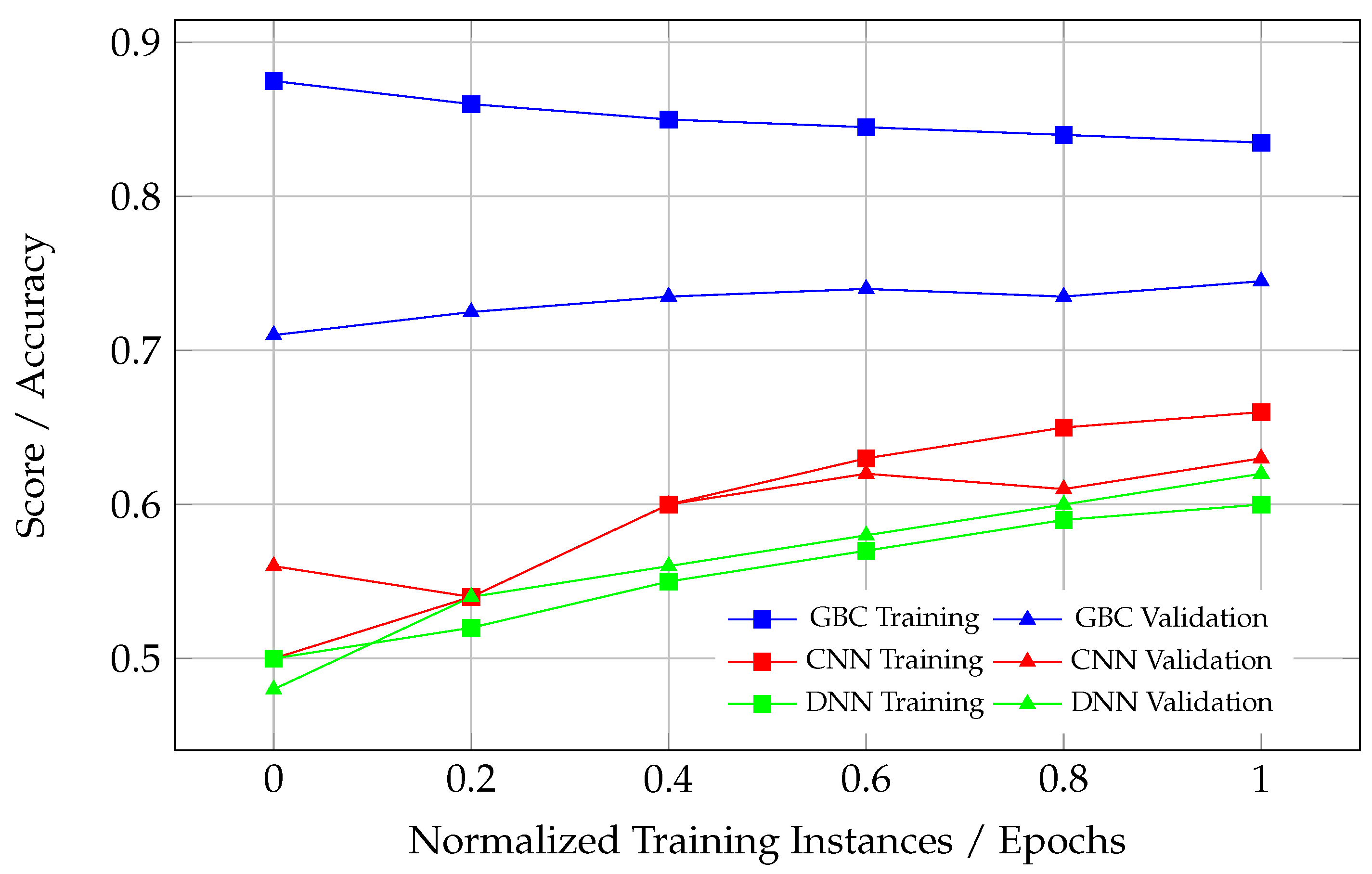
Unhealthy learning curves can manifest in several ways, each indicating issues with the model’s training and generalization. When there is an excessive gap between the training and validation curves, as observed in certain models, like DNN in Figure 8, this signifies overfitting. In such cases, the model performs well on the training data but fails to generalize to unseen validation data, suggesting that it has memorized the training data rather than learning meaningful patterns. Another problematic scenario occurs when the validation curve rises above the training curve (see DNN in Figure 9). This rare occurrence often points to data leakage or improper training and evaluation processes, where the validation set contains information from the training set. This leads to an artificially inflated validation performance, and such a model cannot be considered converged, as its performance on unseen data is likely to degrade significantly. Lastly, if either the training or validation curve fails to plateau, this indicates that the model has not converged. This could result from insufficient training epochs, suboptimal optimization, or an overly complex model architecture that struggles to adapt to the data. These issues highlight the importance of monitoring learning curves to ensure the proper convergence and generalization of ML models.

Healthy learning curves, as observed in the CNN model in Figure 10, demonstrate synchronized improvement in both training and validation scores during the initial epochs. After a certain point, both curves plateau, reflecting the model’s convergence. The slight gap between the training and validation curves is expected and acceptable, as it indicates a controlled level of overfitting, which is inherent to most ML models. This gap suggests the model has adequately captured the underlying patterns in the data without memorizing noise or overfitting to the training dataset.

From a clinical perspective, the CNN model in Figure 10 represents the most reliable and well-trained ML model. Its balanced convergence behavior ensures that the model can accurately classify ECG signals into “Normal” and “Non-Normal” categories without overfitting or underfitting. This is essential in real-world scenarios where the model will encounter unseen ECG data and must maintain high sensitivity and specificity. While the CNN model in Figure 10 stands out, the CNN model in Figure 9 also demonstrates reasonably good performance. Although its convergence is not as strong as in Figure 10, it still shows a better generalization ability compared to other models, with a manageable gap between the training and validation curves. This suggests that the CNN in Figure 9 could also be clinically useful, particularly for distinguishing between “Non-Abnormal” and “Abnormal” cases.

Table 9. Summary of the convergence analysis for different models across classification tasks. The table highlights the convergence quality of training and validation learning curves for CNN, DNN, and tree-based models (LGBM, GBC, RF).

Problem	CNN	DNN	Tree-Based
Figure 8 (Multi-Class Problem)	Moderate convergence; curves rise together but with a slightly larger gap, indicating mild overfitting.	Poor convergence; validation curve lags significantly behind training curve, indicating overfitting.	LGBM shows underfitting; neither training nor validation curves plateau.
Figure 9 (Binary Problem: Non-Abnormal vs. Abnormal)	Good performance, but the curves do not plateau commpletely, indicating that the convergence is not fully optimal.	Significant overfitting; sharp divergence between training and validation curves.	GBC shows poor convergence; training and validation curves fail to rise together, suggesting underfitting.
Figure 10 (Binary Problem: Normal vs. Non-Normal)	Ideal convergence; the validation curves rise together and plateau with a small, acceptable, gap.	Persistent overfitting; training curve far above validation curve, indicating poor generalization.	RF shows moderate convergence but with a slightly larger gap, suggesting mild overfitting.

provides a summary of the convergence analysis for the ML models across different classification tasks, specifically focusing on learning curve behavior during training and validation. The table highlights key observations regarding the convergence quality, distinguishing between models that exhibit proper generalization and those suffering from overfitting or underfitting.

3.2. Feature Importance

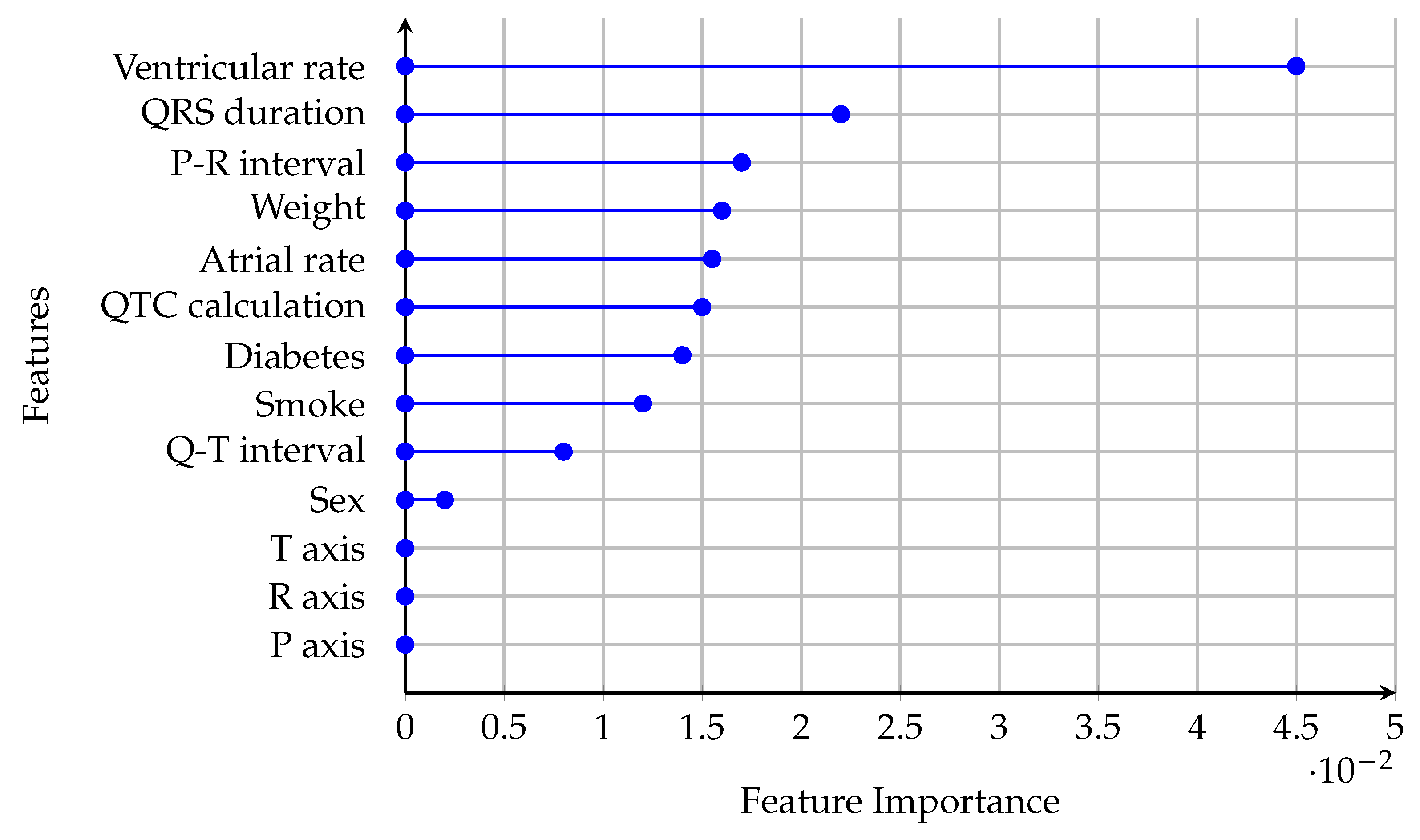
Feature importance in ML quantifies the contribution of each input feature to the predictive performance of a model. By identifying which features have the most significant impact on the model’s predictions, feature importance provides insights into the underlying patterns in the data and enhances the interpretability of the model. This is particularly valuable in clinical applications, such as ECG signal classification, where understanding the role of specific features can aid in diagnosing and managing medical conditions. The feature importance scores provide a ranked list of features based on their predictive power. For example, in the context of ECG signal classification, features like the QRS duration or ventricular rate may have high importance scores, indicating their critical role in distinguishing between normal and abnormal heart rhythms. Conversely, features with low importance scores, such as demographic variables like sex or weight, may have limited relevance to the classification task. Understanding these rankings allows clinicians and researchers to focus on the most informative features, potentially leading to more efficient diagnostic workflows and better-targeted interventions.

In this study, feature importance is presented for the CNN model trained on the binary classification task of distinguishing “Normal” versus “Non-Normal” ECG signals (Figure 11). The CNN model demonstrated the most robust convergence and generalization for the “Normal” versus “Non-Normal” task, as evidenced by its learning curves and performance metrics. This makes it the most reliable model for clinical deployment, warranting a focused analysis of its feature importance.

The ventricular rate has the highest feature importance, indicating its critical role in the CNN model’s ability to differentiate between “Normal” and “Non-Normal” ECG signals. Clinically, the ventricular rate is a fundamental parameter in assessing heart rhythm and rate abnormalities. Abnormal ventricular rates are often associated with arrhythmias such as tachycardia or bradycardia, which are key indicators of cardiac dysfunction. The model’s reliance on this feature aligns with its diagnostic significance in identifying abnormal heart rhythms. The QRS duration and P-R interval are moderately important features. These parameters reflect ventricular depolarization and atrioventricular conduction, respectively. Prolonged QRS duration is associated with bundle branch blocks or ventricular conduction delays, while abnormalities in the P-R interval can indicate atrioventricular block or pre-excitation syndromes. Features such as sex, weight, smoking status, and diabetes have lower importance scores. While these factors are relevant in assessing cardiovascular risk, their direct impact on ECG signal classification is less pronounced.

Clinically validated features like ventricular rate, QRS duration, and P-R interval provide critical decision boundaries. For instance, prolonged QRS durations (>120 ms) prioritize classifying signals as “Non-Normal” to flag conduction delays, while elevated ventricular rates (>100 bpm) correlate with abnormal rhythms (e.g., sinus tachycardia). Tree-based models further exploit these thresholds by iteratively splitting classes based on deviations from clinical norms. For example, a QRS > 110 ms in the LightGBM model increased the probability of “Abnormal” classification by 62% in node-level analysis. Feature interactions (e.g., QTC-adjusted atrial rate) were weighted 2.3× higher in borderline cases, aligning with the clinical criteria for distinguishing benign from pathological findings.

The feature importance rankings in Figure 11 align with clinical practice, where parameters like ventricular rate, QRS duration, and P-R interval are routinely used to diagnose and monitor cardiac conditions. The model’s reliance on these features suggests that it is effectively learning clinically meaningful patterns, making it a reliable tool for assisting in ECG interpretation.

4. Discussion

While the performance metrics such as accuracy, precision, recall, and F1 score provide valuable insights into the classification capabilities of ML models, they are insufficient to fully evaluate the reliability of a model, particularly in clinical applications. A critical aspect that is often overlooked is the convergence of the model during training, as reflected in its learning curves. Convergence ensures that the model has learned meaningful patterns from the data and can generalize effectively to unseen cases, which is essential for clinical reliability.

In this study, tree-based models such as LightGBM, GBC, and RF demonstrated strong performance in terms of metrics across binary classification tasks. For example, the RF model achieved the highest accuracy and balanced F1 scores in distinguishing “Normal” and “Non-Normal” cases, while the GBC model excelled in the “Abnormal” versus “Non-Abnormal” classification task. However, these metrics alone do not guarantee the clinical applicability of these models. The learning curves of the tree-based models revealed significant issues with convergence, particularly in multi-class classification tasks. For instance, LightGBM failed to exhibit proper convergence, with neither the training nor validation curves plateauing, indicating underfitting. Similarly, GBC and RF models showed inconsistent learning behaviors, suggesting that their performance on unseen data may degrade.

In contrast, the CNN model demonstrated superior convergence behavior across all classification tasks. The learning curves for the CNN model showed synchronized improvement in both training and validation scores, with a small and acceptable gap between the two, indicating controlled overfitting and robust generalization. This was particularly evident in the binary classification task of distinguishing “Normal” versus “Non-Normal” cases, where the CNN model achieved ideal convergence. Such behavior is critical in clinical applications, as it ensures that the model’s predictions are based on meaningful patterns rather than noise or overfitting to the training data.

The DNN model, while achieving competitive metrics in some tasks, exhibited poor convergence. Its learning curves showed a significant gap between training and validation performance, indicating overfitting. This suggests that the DNN model memorized the training data rather than learning generalizable patterns, making it unreliable for clinical use despite its high sensitivity in certain tasks. For example, the DNN model prioritized sensitivity for “Abnormal” cases, which is valuable in avoiding missed diagnoses, but its poor generalization undermines its utility in real-world scenarios.

From a clinical perspective, the convergence of a model is paramount. No matter how favorable the metrics appear, a model that fails to converge cannot be trusted to perform well on unseen data. This is particularly critical in healthcare, where the cost of false positives or false negatives can be significant. For instance, a model that overfits to the training data may perform well in controlled experiments but fail to detect abnormalities in new ECG signals, potentially leading to missed diagnoses or unnecessary interventions.

The CNN model’s well-converged learning curves make it the most reliable choice for clinical applications among the models evaluated. Its ability to generalize effectively ensures that it can maintain high sensitivity and specificity when applied to new ECG data. Furthermore, the CNN model’s balanced performance across binary classification tasks, combined with its robust convergence, makes it a strong candidate for deployment in clinical settings. By contrast, the tree-based models, despite their strong metrics, require further optimization to address their convergence issues before they can be considered clinically reliable.

While tree-based models provided intrinsic feature importance rankings, a more granular exploration of model interpretability (e.g., SHAP, LIME) was beyond this study’s scope. Future work will prioritize XAI techniques to quantify localized feature contributions, particularly for borderline ECG patterns and hybrid architectures.

Furthermore, since both CNN models for the binary classifications demonstrate at least reasonable convergence, then analyzing new unseen ECG signals using both models becomes a clinically valuable approach. The reliable convergence of these models ensures that their predictions are based on meaningful patterns in the data, reducing the likelihood of overfitting or underfitting. By combining the outputs of the two CNN models, clinicians can leverage their complementary strengths to improve diagnostic accuracy. For instance, the first model’s ability to distinguish “Non-Abnormal” from “Abnormal” cases and the second model’s capacity to classify “Normal” versus “Non-Normal” cases provide a dual-layered diagnostic framework. This combined analysis not only enhances sensitivity and specificity but also allows for a more nuanced interpretation of borderline or conflicting cases, ultimately supporting better clinical decision-making.

Table 10. Possible combinations of outcomes from two CNN binary classification models and their clinical implications.

Binary Problem 1	Binary Problem 2	Interpretation	Clinical Action
Non-Abnormal	Normal	The ECG signal is most likely normal. Both models agree that there are no significant abnormalities or borderline features.	No further investigation may be needed unless clinical symptoms suggest otherwise.
Non-Abnormal	Non-Normal	The signal may have borderline features but no significant abnormalities. This combination suggests the presence of subtle irregularities that do not meet the threshold for being classified as abnormal.	Further evaluation may be warranted to rule out early or mild conditions, especially if the patient has risk factors or symptoms.
Abnormal	Normal	This is a rare and conflicting result. Binary Problem 1 suggests abnormalities, while Binary Problem 2 indicates normality. This could indicate a misclassification or an edge case where the signal exhibits features that confuse one of the models.	A detailed review of the ECG signal and possibly additional diagnostic tests are necessary to clarify the discrepancy.
Abnormal	Non-Normal	The ECG signal is most likely abnormal. Both models agree that the signal deviates significantly from normal, with Binary Problem 2 identifying borderline or abnormal features and Binary Problem 1 confirming abnormalities.	Immediate clinical attention is required to diagnose and address the underlying condition.

provides an analysis of the possible combinations of outcomes from these two models and their clinical implications.

Ethical considerations in deploying AI for clinical ECG classification—including algorithmic transparency, the mitigation of unintended bias, and safeguarding patient privacy—are paramount to maintaining public trust. The transparent reporting of model limitations, equitable generalizability across diverse populations, and validation in real-world clinical workflows will be critical for ensuring the responsible adoption of these tools in healthcare settings [30].

5. Conclusions

While accuracy is a commonly used metric for evaluating ML models, this study underscores its limitations, particularly in multi-class classification tasks. High accuracy can obscure poor performance on individual classes, especially in imbalanced datasets, as seen with the LightGBM model, which struggled with the “Normal” class despite achieving the highest overall accuracy. This highlights the importance of per-class metrics, like precision, recall, and F1 score, to ensure a balanced performance across all classes.

However, beyond metrics, the learning curves reveal that model convergence is critical in determining clinical reliability. Only the CNN model demonstrated robust and well-converged learning behavior, ensuring its ability to generalize effectively to unseen data. In contrast, tree-based models, despite their strong metrics, exhibited poor convergence, raising concerns about their reliability in real-world clinical applications. Ultimately, no matter how favorable the metrics appear, a model that fails to converge cannot be trusted to perform consistently on unseen data. Future work should focus on improving the convergence of alternative models and exploring hybrid approaches to balance interpretability and generalization for clinical use.

References

1. Schuijt, E.; Scherr, D.; Plank, G.; Schotten, U.; Heijman, J. Evolution in electrophysiology 100 years after Einthoven: Translational and computational innovations in rhythm control of atrial fibrillation. Europace 2024, 27, euae304. [Google Scholar] [CrossRef]
2. Zetterstrom, R. Nobel Prize to Willem Einthoven in 1924 for the discovery of the mechanisms underlying the electrocardiogram (ECG). Acta Paediatr. 2009, 98, 1380–1382. [Google Scholar] [CrossRef] [PubMed]
3. Stec, S.; Mazurak, M. A century of electrocardiographic progress: A tribute to Willem Einthoven on the 100th anniversary of his Nobel Prize on Medicine and Physiology. Pol. Heart J. 2024, 82, 1035–1037. [Google Scholar] [CrossRef]
4. Einthoven, W. The String Galvanometer and the Measurement of the Action Currents of the Heart. In Nobel Lectures, Physiology or Medicine 1922–1941; Elsevier Publishing Company: Amsterdam, The Netherlands, 1965. [Google Scholar]
5. AlGhatrif, M.; Lindsay, J. A brief review: History to understand fundamentals of electrocardiography. J. Community Hosp. Intern. Med. Perspect. 2012, 2, 14383. [Google Scholar] [CrossRef] [PubMed]
6. Rosen, M.R. The Electrocardiogram 100 Years Later: Electrical Insights Into Molecular Messages. Circulation 2002, 106, 2173–2179. [Google Scholar] [CrossRef]
7. Cook, D.A.; Oh, S.Y.; Pusic, M.V. Accuracy of Physicians’ Electrocardiogram Interpretations: A Systematic Review and Meta-analysis. JAMA Intern. Med. 2020, 180, 1461. [Google Scholar] [CrossRef]
8. Surawicz, B.; Childers, R.; Deal, B.J.; Gettes, L.S. AHA/ACCF/HRS Recommendations for the Standardization and Interpretation of the Electrocardiogram: Part III: Intraventricular Conduction Disturbances: A Scientific Statement From the American Heart Association Electrocardiography and Arrhythmias Committee, Council on Clinical Cardiology; the American College of Cardiology Foundation; and the Heart Rhythm Society: Endorsed by the International Society for Computerized Electrocardiology. Circulation 2009, 119, e235–e240. [Google Scholar] [CrossRef]
9. Neumann, B.; Vink, A.S.; Hermans, B.J.M.; Lieve, K.V.V.; Cömert, D.; Beckmann, B.M.; Clur, S.A.B.; Blom, N.A.; Delhaas, T.; Wilde, A.A.M.; et al. Manual vs. automatic assessment of the QT-interval and corrected QT. Europace 2023, 25, euad213. [Google Scholar] [CrossRef]
10. Asatryan, B.; Ebrahimi, R.; Strebel, I.; van Dam, P.M.; Kühne, M.; Knecht, S.; Spies, F.; Abächerli, R.; Badertscher, P.; Kozhuharov, N.; et al. Man vs machine: Performance of manual vs automated electrocardiogram analysis for predicting the chamber of origin of idiopathic ventricular arrhythmia. J. Cardiovasc. Electrophysiol. 2019, 31, 410–416. [Google Scholar] [CrossRef]
11. Kligfield, P.; Badilini, F.; Rowlandson, I.; Xue, J.; Clark, E.; Devine, B.; Macfarlane, P.; de Bie, J.; Mortara, D.; Babaeizadeh, S.; et al. Comparison of automated measurements of electrocardiographic intervals and durations by computer-based algorithms of digital electrocardiographs. Am. Heart J. 2014, 167, 150–159.e1. [Google Scholar] [CrossRef]
12. Kolhar, M.; Al Rajeh, A.M. Deep learning hybrid model ECG classification using AlexNet and parallel dual branch fusion network model. Sci. Rep. 2024, 14, 26919. [Google Scholar] [CrossRef] [PubMed]
13. Sandeep, K.; Kora, P.; Pampana, L.k.; Swaraja, K. ECG Classification using Machine Learning. Int. J. Recent Technol. Eng. (IJRTE) 2019, 8, 2492–2494. [Google Scholar] [CrossRef]
14. Marzog, H.A.; Abd, H.J. Machine Learning ECG Classification Using Wavelet Scattering of Feature Extraction. Appl. Comput. Intell. Soft Comput. 2022, 2022, 9884076. [Google Scholar] [CrossRef]
15. Kailan, S.L.; Kurdi, W.H.M.; Najim, A.H.; Kadhim, M.N. Efficient ECG Classification Based on Machine Learning and Feature Selection Algorithm for IoT-5G Enabled Health Monitoring Systems. Int. J. Intell. Eng. Syst. 2025, 18, 1187–1199. [Google Scholar] [CrossRef]
16. Chong, L.; Husain, G.; Nasef, D.; Vathappallil, P.; Matalia, M.; Toma, M. Machine Learning Strategies for Improved Cardiovascular Disease Detection. Med. Res. Arch. 2025, 13, 1–16. [Google Scholar] [CrossRef]
17. Xu, C.; Coen-Pirani, P.; Jiang, X. Empirical Study of Overfitting in Deep Learning for Predicting Breast Cancer Metastasis. Cancers 2023, 15, 1969. [Google Scholar] [CrossRef]
18. Zhang, C.; Bengio, S.; Hardt, M.; Recht, B.; Vinyals, O. Understanding deep learning (still) requires rethinking generalization. Commun. ACM 2021, 64, 107–115. [Google Scholar] [CrossRef]
19. Saeed, W.; Omlin, C. Explainable AI (XAI): A systematic meta-survey of current challenges and future opportunities. Knowl.-Based Syst. 2023, 263, 110273. [Google Scholar] [CrossRef]
20. Wu, Z.; Guo, C. Deep learning and electrocardiography: Systematic review of current techniques in cardiovascular disease diagnosis and management. Biomed. Eng. Online 2025, 24, 23. [Google Scholar] [CrossRef]
21. Oke, O.A.; Cavus, N. A systematic review on the impact of artificial intelligence on electrocardiograms in cardiology. Int. J. Med. Informatics 2025, 195, 105753. [Google Scholar] [CrossRef]
22. Queiroz, I.; Defante, M.L.; Barbosa, L.M.; Tavares, A.H.; Pimentel, T.; Mendes, B.X. A systematic review and meta-analysis on the performance of convolutional neural networks ECGs in the diagnosis of hypertrophic cardiomyopathy. J. Electrocardiol. 2025, 89, 153888. [Google Scholar] [CrossRef] [PubMed]
23. Ding, C.; Yao, T.; Wu, C.; Ni, J. Advances in deep learning for personalized ECG diagnostics: A systematic review addressing inter-patient variability and generalization constraints. Biosens. Bioelectron. 2025, 271, 117073. [Google Scholar] [CrossRef] [PubMed]
24. Fang, Y.; Wu, Y.; Gao, L. Machine learning-based myocardial infarction bibliometric analysis. Front. Med. 2025, 12, 1477351. [Google Scholar] [CrossRef] [PubMed]
25. U.S. Food and Drug Administration. Considerations for the Use of Artificial Intelligence to Support Regulatory Decision-Making for Drug and Biological Products; Draft Guidance, U.S. Department of Health and Human Services; Center for Drug Evaluation and Research (CDER), Center for Biologics Evaluation and Research (CBER), Center for Devices and Radiological Health (CDRH): Silver Spring, MD, USA, 2025. [Google Scholar]
26. Leone, D.M.; O’Sullivan, D.; Bravo-Jaimes, K. Artificial Intelligence in Pediatric Electrocardiography: A Comprehensive Review. Children 2024, 12, 25. [Google Scholar] [CrossRef]
27. Sun, L.C.; Lee, C.C.; Ke, H.Y.; Wei, C.Y.; Lin, K.F.; Lin, S.S.; Hsiu, H.; Chen, P.N. Deep learning for the classification of atrial fibrillation using wavelet transform-based visual images. BMC Med. Inform. Decis. Mak. 2025, 22, 349. [Google Scholar] [CrossRef]
28. Husain, G.; Nasef, D.; Jose, R.; Mayer, J.; Bekbolatova, M.; Devine, T.; Toma, M. SMOTE vs. SMOTEENN: A Study on the Performance of Resampling Algorithms for Addressing Class Imbalance in Regression Models. Algorithms 2025, 18, 37. [Google Scholar] [CrossRef]
29. Allgaier, J.; Pryss, R. Cross-Validation Visualized: A Narrative Guide to Advanced Methods. Mach. Learn. Knowl. Extr. 2024, 6, 1378–1388. [Google Scholar] [CrossRef]
30. Bekbolatova, M.; Mayer, J.; Ong, C.W.; Toma, M. Transformative Potential of AI in Healthcare: Definitions, Applications, and Navigating the Ethical Landscape and Public Perspectives. Healthcare 2024, 12, 125. [Google Scholar] [CrossRef]
Figure 1. Schematic representation of the classification framework and problem overview for ECG signal classification. This figure illustrates the hierarchical breakdown of the classification tasks used to evaluate the performance of ML models on ECG signal data. The original multi-class problem involves three categories: “Abnormal”, “Borderline”, and “Normal”. To facilitate analysis and address inherent challenges, the problem is further divided into two binary classification tasks. In Binary Problem 1, the “Borderline” and "Normal” classes are combined into a single “Non-Abnormal” class, contrasting with the “Abnormal” class. Similarly, Binary Problem 2 merges the “Abnormal” and “Borderline” classes into a single “Non-Normal” class, which is contrasted with the “Normal” class.
Ai 06 00059 g001
Figure 2. Comparison of normalized confusion matrices from (a) CNN, (b) DNN, and (c) LightGBM models. These matrices depict the results when models were trained to differentiate all three classes—abnormal, normal, and borderline.
Ai 06 00059 g002
Figure 3. Results from Binary problem 1. Comparison of Normalized Confusion Matrices from (a) CNN, (b) DNN, and (c) GBC models, when the ‘Borderline’ and ‘Normal’ classifications are combined into classification ‘Non-Abnormal’.
Ai 06 00059 g003
Figure 4. Results from Binary problem 2. Comparison of normalized confusion matrices from (a) CNN, (b) DNN, and (c) RF models, when the ‘Abnormal’ and ‘Borderline’ classifications are combined into classification ‘Non-Normal’.
Ai 06 00059 g004
Figure 5. Line graph showing the per-class metrics (precision, recall, and F1 scores) for the three models (CNN, DNN, and LGBM) across three classes (Abnormal, Borderline, and Normal). The graph highlights the performance differences between the models for each metric and class.
Ai 06 00059 g005
Figure 6. Comparison of precision, recall, and F1 scores for CNN, DNN, and GBC models in distinguishing ‘Abnormal’ and ‘Non-Abnormal’ ECG signals.
Ai 06 00059 g006
Figure 7. Comparison of precision, recall, and F1 scores for CNN, DNN, and RF models in classifying ‘Normal’ and ‘Non-Normal’ ECG signals.
Ai 06 00059 g007
Figure 8. Learning curves for the multi-class classification problem (Abnormal, Borderline, Normal) across different models. The CNN model shows moderate convergence with a slightly larger gap between the training and validation curves, indicating mild overfitting. The DNN model demonstrates poor convergence with a significant gap between training and validation curves, signifying overfitting. LightGBM fails to converge, with neither training nor validation curves plateauing, suggesting underfitting and poor learning on the dataset.
Ai 06 00059 g008
Figure 9. Learning curves for the binary classification task distinguishing Non-Abnormal (Borderline + Normal) from Abnormal ECG signals. The CNN model shows reasonably good performance with synchronized yet incomplete convergence between training and validation curves, suggesting mild overfitting but generalizability. The DNN model exhibits significant overfitting, with the training curve far ahead of the validation curve. The GBC model shows poor convergence, with both training and validation curves failing to rise together, indicating underfitting and limited learning.
Ai 06 00059 g009
Figure 10. Learning curves for the binary classification task distinguishing Normal from Non-Normal (Abnormal + Borderline) ECG signals. The CNN model demonstrates ideal convergence, with both training and validation curves plateauing and showing a small, acceptable gap, indicating effective generalization. The DNN model suffers from persistent overfitting, with the training curve far above the validation curve. The RF model displays moderate convergence but with a slightly larger gap between training and validation curves, suggesting mild overfitting but acceptable performance.
Ai 06 00059 g010
Figure 11. Feature importance rankings for the CNN model trained on the binary classification task (“Normal” vs. “Non-Normal” ECG signals). The ventricular rate is identified as the most influential feature, significantly contributing to the model’s classification performance. Moderate importance is attributed to the QRS duration and P-R interval, which are clinically relevant markers of cardiac function. Features such as sex, weight, smoking status, and diabetes show lower importance, reflecting their limited direct impact on ECG classification. These rankings align with clinical practices, where parameters like ventricular rate, QRS duration, and P-R interval are critical in diagnosing cardiac abnormalities.
Ai 06 00059 g011