AI-Driven Threat Hunting in Enterprise Networks Using Hybrid CNN-LSTM Models for Anomaly Detection

Abstract

Objectives: This study aims to present an AI-driven threat-hunting framework that automates both hypothesis generation and hypothesis validation through a hybrid deep learning model that combines Convolutional Neural Networks (CNN) with Long Short-Term Memory (LSTM) networks. The objective is to operationalize proactive threat hunting by embedding anomaly detection within a structured workflow, improving detection performance, reducing analyst workload, and strengthening overall security posture. Methods: The framework begins with automated hypothesis generation, in which the model analyzes network flows, telemetry data, and logs sourced from IoT/IIoT devices, Windows/Linux systems, and interconnected environments represented in the TON_IoT dataset. Deviations from baseline behavior are detected as potential threat indicators, and hypotheses are prioritized according to anomaly confidence scores derived from output probabilities. Validation is conducted through iterative classification, where CNN-extracted spatial features and LSTM-captured temporal features are jointly used to confirm or refute hypotheses, minimizing manual data pivoting and contextual enrichment. Principal Component Analysis (PCA) and Recursive Feature Elimination with Random Forest (RFE-RF) are employed to extract and rank features based on predictive importance. Results: The hybrid model, trained on the TON_IoT dataset, achieved strong performance metrics: 99.60% accuracy, 99.71% precision, 99.32% recall, an AUC of 99%, and a 99.58% F1-score. These results outperform baseline models such as Random Forest and Autoencoder. By integrating spatial and temporal feature extraction, the model effectively identifies anomalies with minimal false positives and false negatives, while the automation of the hypothesis lifecycle significantly reduces analyst workload. Conclusions: Automating threat-hunting processes through hybrid deep learning shifts organizations from reactive to proactive defense. The proposed framework improves threat visibility, accelerates response times, and enhances overall security posture. The findings offer valuable insights for researchers, practitioners, and policymakers seeking to advance AI adoption in threat intelligence and enterprise security.

1. Introduction

The rapid digitization of business operations has ushered in unprecedented opportunities for innovation, scalability, and operational efficiency. However, this transformation has also significantly expanded the attack surface of organizations through increasingly complex and interconnected technological infrastructures [1]. The widespread adoption of internetworking devices, cloud services, and Internet of Things (IoT) technologies has introduced multiple vectors for exploitation, complicating efforts to secure digital assets [2,3].

As the cyber threat landscape continues to evolve, organizations face mounting challenges in maintaining robust security postures. Traditional security mechanisms such as firewalls, antivirus software, and intrusion detection systems are inherently reactive and often insufficient against emerging threats that exploit vulnerabilities before detection and response can occur [1]. These legacy systems rely heavily on known threat signatures, limiting their capacity to identify novel or sophisticated attacks in real time [4]. Consequently, there is a growing shift toward proactive cybersecurity strategies, notably threat hunting, which aims to detect and mitigate both known and unknown threats before they materialize [5].

Threat hunting is a dynamic and iterative process involving the generation, monitoring, and refinement of threat hypotheses. It operates under the assumption that adversaries may already reside within the network, prompting analysts to validate hypotheses through active investigation and anomaly detection [6]. Unlike traditional security tools, threat hunting enables pre-emptive identification of malicious activity, offering a more aggressive and anticipatory defense posture [7]. Hypotheses are typically informed by threat intelligence and historical data, serving as educated guesses to explain potential intrusions or suspicious behavior [3]. This proactive stance is critical, as cyber-attacks frequently bypass signature-based detection and do not always trigger conventional alerts [4].

To enhance the effectiveness of threat hunting, organizations increasingly leverage machine learning (ML) algorithms capable of processing vast volumes of network and system data. These algorithms identify anomalous patterns and deviations from baseline behavior, improving detection accuracy over time through continuous learning. ML-driven threat hunting facilitates rapid classification of threats, enabling timely response and mitigation [8]. By analyzing historical data and categorizing incidents, AI-based systems significantly reduce response times and limit the impact of cyber-attacks.

Advanced techniques, such as natural language processing and predictive analytics, further empower security tools to detect subtle indicators of compromise. AI-powered systems can autonomously monitor network traffic, identify anomalies, and forecast potential threats before they escalate [9]. Technologies, including deep learning and pattern recognition, have become instrumental in developing intelligent systems capable of real-time threat detection and adaptive response [10]. These autonomous platforms not only strengthen threat intelligence but also accelerate incident response, thereby minimizing organizational exposure to cyber risks [8].

Traditionally, hypotheses are crafted manually by security analysts, who rely on their expertise to interpret vast amounts of network data and identify potential signs of compromise. However, as Nour et al. (2023) [11] highlight, this process is both time-consuming and highly dependent on specialist knowledge, which is not always available. In large enterprise environments, where data volumes are immense and threats are increasingly sophisticated, manual hypothesis generation quickly becomes unsustainable. Equally critical is the validation and verification of these hypotheses, which determines whether a threat truly exists and reveals the tactics, techniques, and procedures (TTPs) used by attackers. Yet, as Jadidi and Lu (2021) [4] note, manual validation often overlooks the reliability and quality of the hypotheses themselves, leading to delayed responses and missed threats.

As a result, manual hypothesis generation and validation remain major bottlenecks in the threat hunting process—slowing detection, increasing the risk of human error, and limiting organizational agility in responding to emerging threats. Although prior research has advanced threat hunting through machine learning, graph-based approaches, and proactive frameworks, these methods remain constrained by reliance on static datasets, the continued need for manual hypothesis generation, and limited integration of heterogeneous data sources. Moreover, high-performing ML models often lack explainability, which hinders trust and adoption in real-world enterprise environments. This creates a clear methodological gap: the absence of an automated, standardized, and interpretable and standardized threat hunting methodology that unifies hypothesis generation, validation, and proactive detection across diverse and evolving data sources.

This study aims to automate the generation and validation of threat hypotheses using deep learning techniques, ultimately improving detection speed, reducing false positives, and strengthening the cybersecurity posture of the enterprise. Hence, the study makes the following contribution:

• Introduce a hybrid CNN-LSTM model that automates both hypothesis generation and validation, reducing reliance on manual analyst input.
• Implement TON_IoT to automate hypothesis generation and validation in the threat hunting process
• Confidence-based hypothesis prioritization, transforming raw anomaly scores into actionable, ranked threat leads for SOC triage
• Enhance the framework with PCA and RFE-RF for interpretable feature selection and applied imbalance-handling techniques (SMOTE, stratified sampling) to improve robustness on IoT/IIoT datasets.

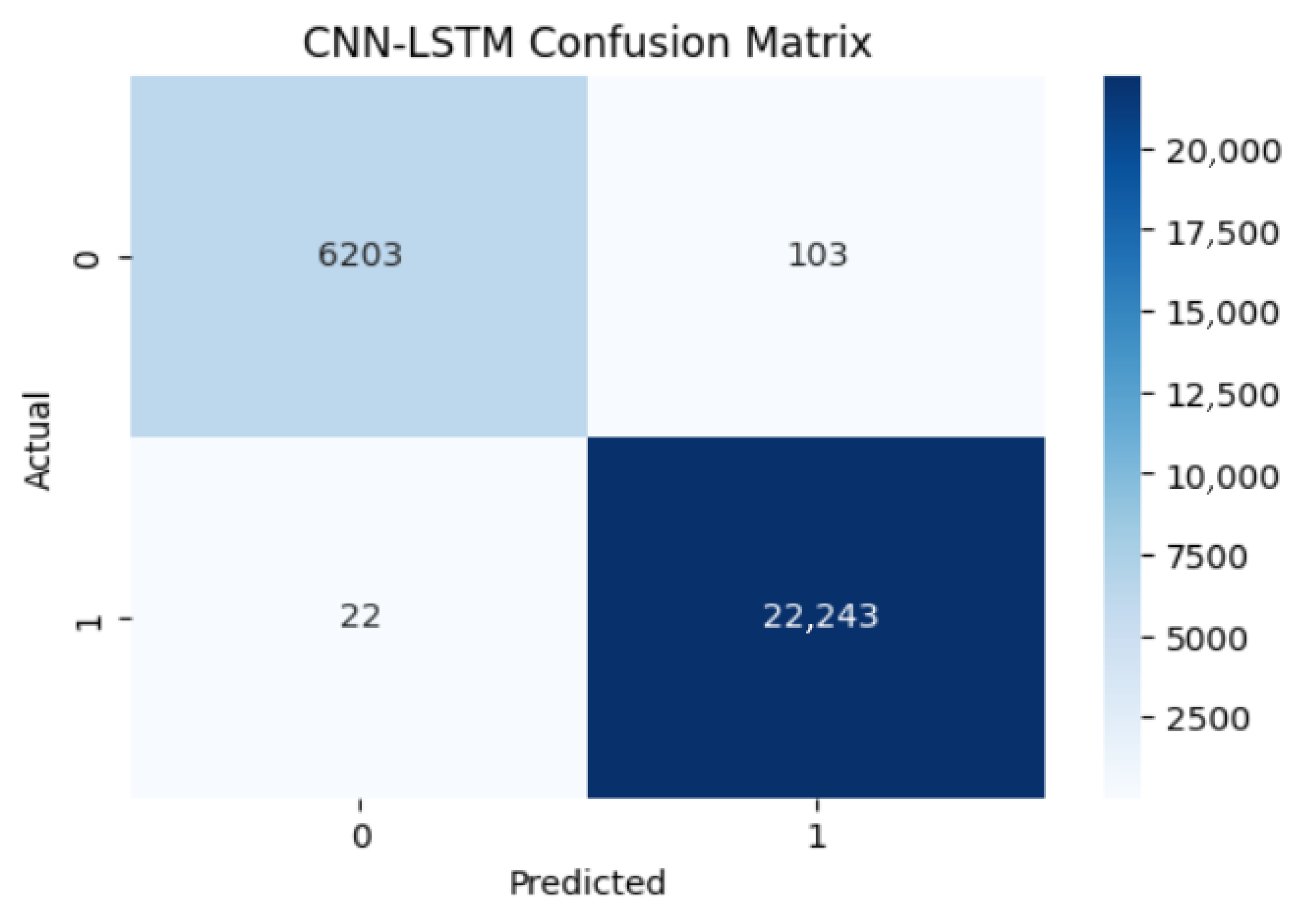
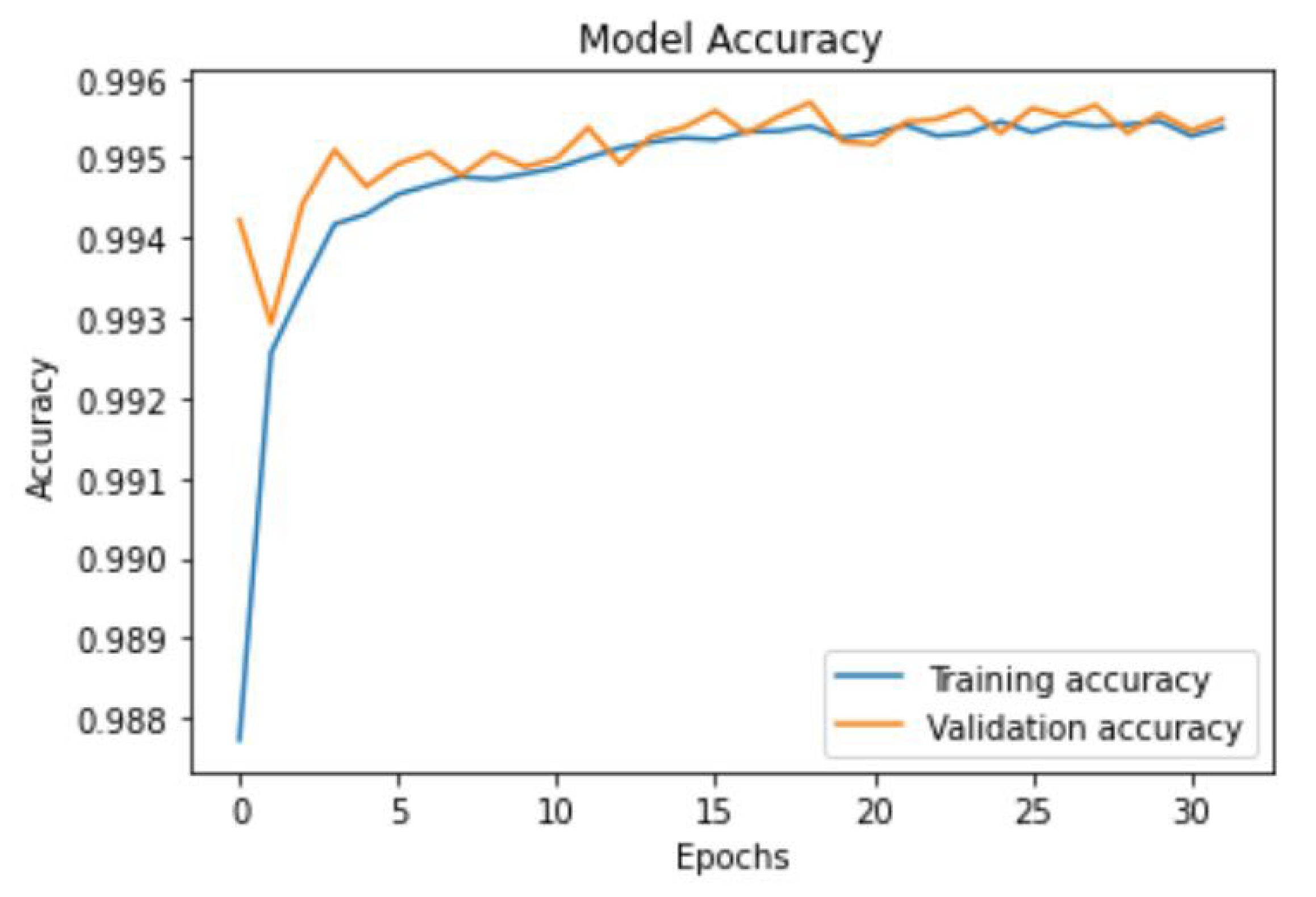
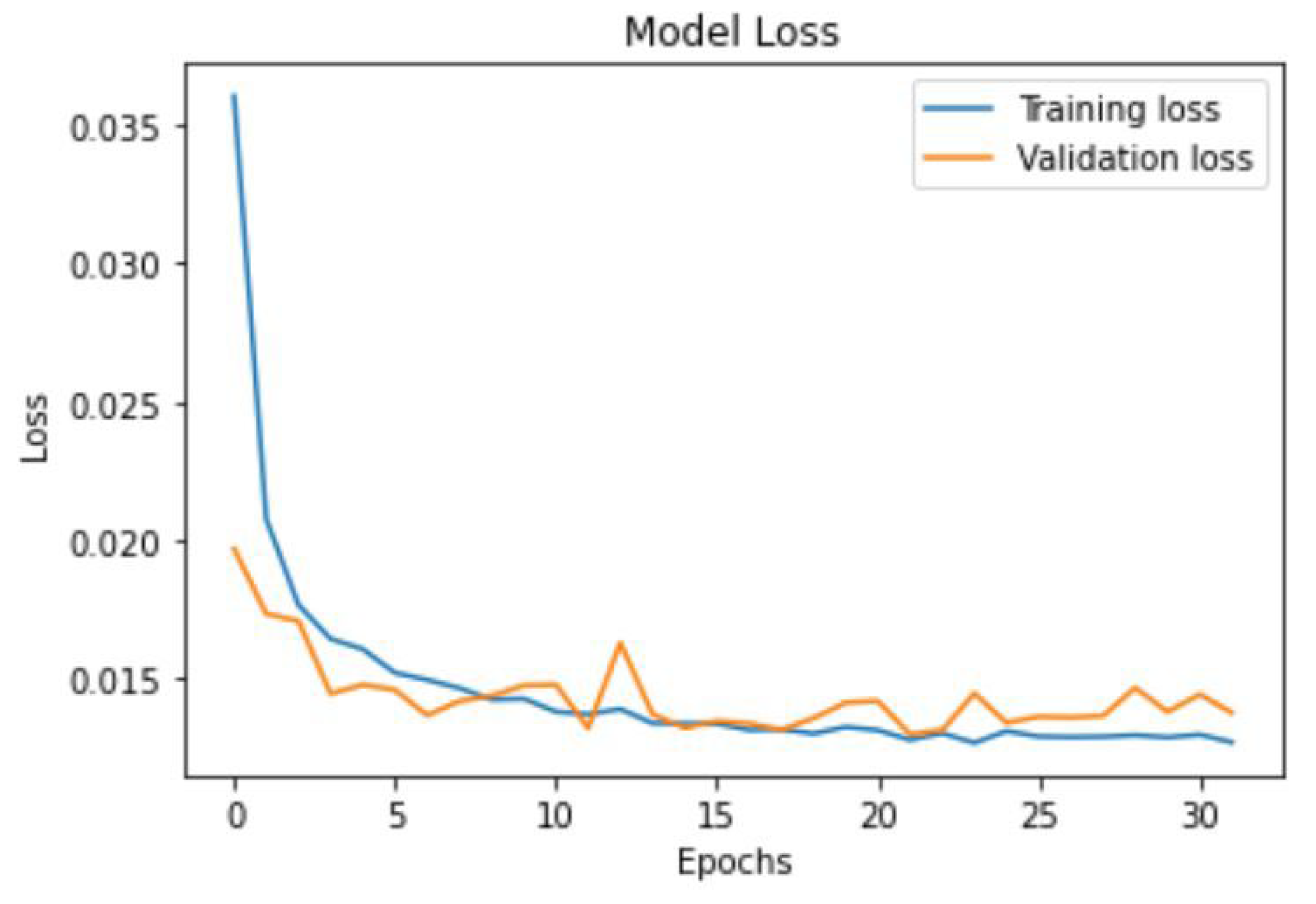
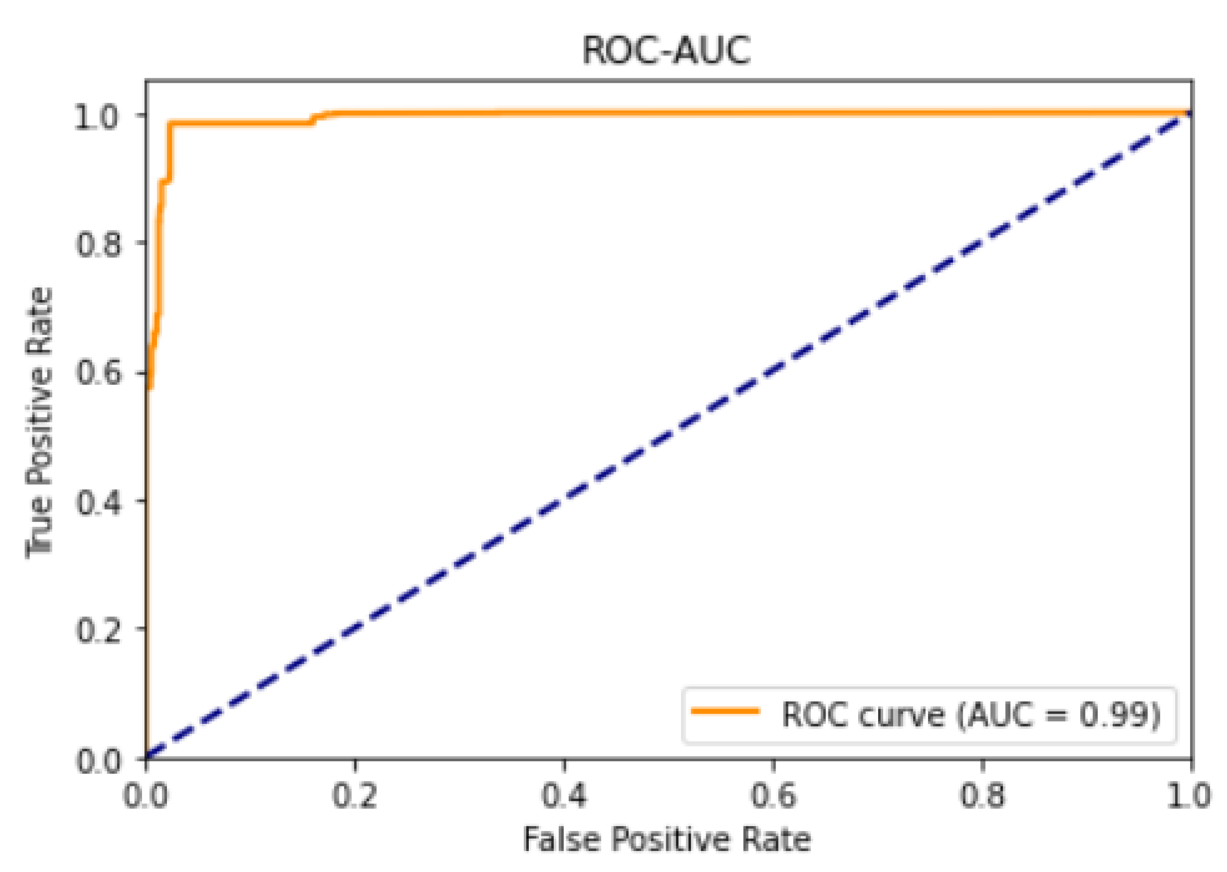
The structure of this paper is as follows: Section 2 reviews relevant literature on AI-based threat detection and hybrid deep learning models. Section 3 outlines the proposed methodology, including the CNN-LSTM architecture and feature selection techniques. Section 4 describes the experimental setup, and Section 5 presents performance evaluation using the TON_IoT dataset. This section also presents the empirical findings, including confusion matrices, accuracy and loss curves, ROC curves, and comparative performance analyses. Section 6 concludes the study with key findings, and Section 7 highlights directions for future research.

2. Related Work

Threat hunting has emerged as a proactive approach to cybersecurity, aiming to identify advanced persistent threats (APTs) and stealthy intrusions that evade traditional detection mechanisms. Across the literature, three recurring themes can be observed: the centrality of hypothesis generation, the increasing role of AI/ML in automation, and the limitations in scalability, data integration, and explainability.

2.1. Threat Hunting Foundations and Hypothesis Generation

Several studies highlight the role of hypotheses as the starting point of effective threat hunting. Mahboubi et al. (2024) [3] emphasise the need to formulate hypotheses before investigations, noting that traditional measures remain important but the integration of AI/ML enables proactive identification of threats. Similarly, Nour et al. (2023) [6] stress that hypothesis generation in current practice is manual and analyst-driven, which is both time-consuming and dependent on scarce expertise. This manual approach represents a significant bottleneck in enterprise environments with high data volumes. Studies such as Jadidi and Lu (2021) [4] and Yi and Kim (2024b) [12] propose structured frameworks for hypothesis generation (e.g., combining MITRE ATT&CK and diamond models, or multi-step evaluation of IT assets), yet these often suffer from limited automation and difficulties in validation. Works by Elitzur et al. (2019) [13], Neto and Dos Santos (2020) [14], and Kaiser et al. (2023) [15] experiment with knowledge graphs and structured threat intelligence to automate attack hypothesis generation. However, challenges remain around graph completeness, feature richness, and mapping behaviours to precise adversarial techniques. These studies collectively highlight the urgent need for automated, reliable, and explainable hypothesis generation and validation mechanisms.

2.2. Proactive Threat Hunting and AI-Driven Models

A second strand of literature focuses on the use of machine learning and deep learning for proactive threat hunting. Nursidiq and Lim (2023) [2] and Kulkarni et al. (2023) [5] propose frameworks that collect and analyse traffic patterns using MITRE ATT&CK, improving detection of unknown threats. However, both frameworks rely on manual validation, slowing response times. The adoption of ML/DL models is well demonstrated in Kansal and Saxena (2024) [1], who show that deep learning achieves higher accuracy than traditional methods and can detect complex patterns indicative of APTs. Sindiramutty (2023) [8] similarly highlights AI’s role in shifting threat intelligence from reactive to proactive detection, while also pointing to interpretability and ethical challenges. Gao et al. (2021) [16] propose THREATRAPTOR, an NLP-based system using open-source threat intelligence, achieving high accuracy in extracting IOCs but facing limitations in handling more complex entities such as threat actors or security tools. Collectively, these works illustrate progress in proactive models but reveal limitations in terms of manual steps, static datasets, and insufficient automation of validation.

2.3. Deep Learning for Anomaly Detection in Threat Hunting

Deep learning techniques particularly CNN and LSTM hybrids have been widely explored for intrusion detection and anomaly detection in network traffic. Abdallah et al. (2021) [17], Halbouni et al. (2022a) [18], and Akkepalli and Sagar (2024) [19] demonstrate that CNN-LSTM and CNN-BiLSTM architectures achieve high accuracy (up to 99%) across datasets such as CIC-IDS2017, UNSW-NB15, and InSDN. However, all report challenges with imbalanced datasets, high false alarm rates, or low detection rates for certain attack categories (e.g., web attacks, worms, and backdoors). Benaddi et al. (2023) [20] confirm CNN-LSTM’s strength in IoT networks, but note limitations compared to alternative models such as SMOTE-DRNN. Gupta et al. (2024) [21] address the black-box nature of DL by incorporating explainable AI (XAI), combining ensemble learning with interpretability to enhance analyst trust.

More recent studies further validate these findings. Agbor et al. (2025) [22] proposed a hybrid CNN–BiLSTM–DNN framework for IoT threat detection, achieving high detection accuracy while mitigating false alarms through deep feature fusion. Cimino et al. (2025) [23] introduced SIGFRID, an unsupervised and platform-agnostic interference detection system for IoT automation, demonstrating the viability of non-intrusive DL-based anomaly detection. Dritsas et al. (2025) [24] provided a comprehensive survey on IoT cybersecurity, highlighting the growing role of deep learning architectures while emphasizing persistent challenges such as scalability, interpretability, and real-time adaptability. These studies indicate that while CNN/LSTM models perform well in controlled settings, improvements are still needed in false positive reduction, class imbalance handling, and explainability for real-world deployment.

Table 1. Summary of Related Work in AI-Driven Threat Hunting and Anomaly Detection.

Theme	Key Studies	Methods/Approaches	Contributions	Limitations
Threat Hunting Foundations & Hypothesis Generation	[3,4,6,12,13,14,15]	Knowledge graphs, MITRE ATT&CK, diamond models, structured frameworks	Automated hypothesis generation; proactive threat identification	Manual processes; graph incompleteness; validation difficulties; expertise dependency
Proactive Threat Hunting & AI-Driven Models	[1,2,5,8]	Traffic pattern analysis, deep learning, NLP-based threat intelligence	Detection of unknown threats; shift from reactive to proactive; high IOC extraction accuracy	Manual validation; static datasets; interpretability challenges
Deep Learning for Anomaly Detection	[17,18,19,20,21,22,23,24]	CNN-LSTM hybrids, BiLSTM, ensemble learning, XAI integration	High accuracy (up to 99%); improved IoT/SDN anomaly detection; explainability enhancements	Imbalanced datasets; false alarms; scalability issues; real-time adaptability limitations

provides an overview of related work in AI-driven threat hunting and anomaly detection, highlighting key themes, representative studies, methodological approaches, primary contributions, and associated limitations.

2.4. Dataset Limitations and Deployment Challenges

A recurring limitation across the reviewed studies is the reliance on static, benchmark datasets. While these enable controlled evaluation, they fail to capture the evolving nature of enterprise and IoT/IIoT environments. Mahboubi et al. (2024) [3] highlight the scarcity of high-quality labelled data, with the latter further noting difficulties in reproducing real-time environments due to data protection restrictions. In terms of deployment, most studies stop at model evaluation, with few addressing real-world integration into enterprise monitoring systems. This limits the practical adoption of otherwise high-performing ML/DL approaches.

3. Methodology

The proposed hybrid model integrates Convolutional Neural Networks (CNN) and Long Short-Term Memory (LSTM) networks to enhance the classification accuracy of normal versus anomalous network traffic. CNNs are supervised learning algorithms known for their robustness in computer vision and efficiency in detecting malicious activity due to their ability to learn directly from data and capture spatial features [20,21,25]. They mitigate parameter explosion through weight sharing, accelerating training processes. LSTMs, a variant of Recurrent Neural Networks (RNNs), are designed for time-series data and address the vanishing gradient problem by retaining relevant long-term dependencies through internal loops [17,26].

As baseline models, Random Forest Classifier (RFC) and Autoencoder (AE) are employed. RFC is a supervised ensemble method that constructs multiple decision trees and aggregates their predictions to reduce overfitting and improve accuracy. It handles high-dimensional data efficiently, is resistant to noise and outliers, and uses bootstrap sampling and voting mechanisms to enhance generalisation [27,28]. Its decision-making is guided by the Gini Index Formula (1):

$$Gini Index \left(d\right)=1-{\sum }_{i=1}^m{P}_i^2$$

(1)

Pi is the proportion of the number of attributes in each class, and m is the number of each class. The feature that has the lowest total Gini Index value will be the root node in the tree. The total Gini Index Formula (2) at an internal node:

$$Tot.Gini index \left(K\right)={\displaystyle \frac{T_1}{T}}Gini Index (D1)+{\displaystyle \frac{T_2}{T}}Gini Index (D2)$$

(2)

where T₁ is the total records belonging to the first class, T₂ is the total records belonging to the second class, and T is the total records of all classes.

The Autoencoder (AE), an unsupervised neural network, is used to detect anomalies (Equation (4)) by learning and reconstructing normal traffic patterns. Deviations from these patterns are flagged based on reconstruction error, using a threshold derived from the Mean Squared Error (MSE) in Formula (3) [29,30,31]. The AE architecture consists of an encoder and decoder, trained to minimise:

$$MSE={\displaystyle \frac{1}{n}}{\sum }_{i=1}^n\left|\right|x_i-x_i^{\prime }{\left|\right|}^2$$

(3)

where x_i is the original input, $x_i^{\prime }$ is the reconstructed output and n is the number of data points.

$$Anomaly=\left\{\begin{array}{c}1 MSE>T\\ 0 MSE\le T\end{array}\right.$$

(4)

where 1 denotes an anomaly and 0 represents normal traffic.

3.1. Data Collection

To train the proposed model, an appropriate dataset is required. The network traffic dataset is obtained from the publicly available TON_IoT dataset. The TON_IoT dataset is generated from a variety of data sources collected from telemetry datasets of IoT and IIoT systems, including data of connected devices such as Windows and Linux operating systems, as well as network traffic from the IIoT system [22]. The full TON_IoT dataset contains 22,339,021 instances, with 21,542,641 attack samples and 796,380 normal samples, indicating a severe class imbalance (96.43% attack vs. 3.57% normal). The attack samples encompass nine categories: scanning, injection, ransomware, backdoor, man in the middle (MITM), distributed denial of service (DDoS), denial of service (DoS), cross-site scripting (XSS), and password attacks. While the exact distribution of samples across these specific attack categories in the full dataset is not detailed here, the overwhelming majority of samples being attack instances confirms the dataset’s significant imbalance, with normal traffic representing only 3.57% of the total. For this study, the network train-test subset (train_test_network.csv), comprising 211,043 instances initially, was used. This subset maintains a similar imbalance pattern to the full dataset, with the majority of samples being attack instances across the nine attack categories mentioned. After preprocessing (as detailed in Section 3.1.1), the dataset was reduced to 190,474 instances while preserving the class imbalance characteristics. The dataset includes a label column with two classes for binary classification: normal (0) and anomalous (1). To address the severe class imbalance observed in both the full dataset and the train-test subset, synthetic minority oversampling technique (SMOTE) was applied during preprocessing to balance class representation, as described in the following section.

3.1.1. Pre-Processing

The dataset, initially comprising 211,043 instances and 44 features, was loaded using Pandas and cleaned to ensure quality for machine learning classification. Features such as source/destination ports and IP addresses were removed due to their limited predictive value and risk of over-fitting. After eliminating duplicates and redistributing missing (‘-’) values across categorical classes, the dataset was reduced to 190,474 instances and 40 features. To address the severe class imbalance inherent in the TON_IoT dataset (96.43% attack vs. 3.57% normal in the full dataset, and similarly imbalanced in the 190,474-instance subset), SMOTE (Synthetic Minority Over-sampling Technique) was applied to generate synthetic samples of the minority class (normal traffic), effectively balancing the dataset for training. Stratified sampling was also employed during dataset splitting to maintain class proportions across train, validation, and test sets. After SMOTE augmentation and feature selection (PCA retaining 95% variance and RFE-RF selecting the top 20 most predictive features), the final dataset distribution is as follows:

• Training set: 1,333,331 samples × 20 features (95.89% of total)
• Validation set: 28,572 samples × 20 features (2.05% of total)
• Test set: 28,571 samples × 20 features (2.05% of total)
• Total: 1,390,474 samples × 20 features

Due to SMOTE augmentation, the final training dataset achieves approximately balanced class distribution (roughly 50% normal vs. 50% attack samples), enabling the hybrid CNN-LSTM model to learn effectively from both classes without bias toward the dominant attack category.

Table 2. Distribution of the TON_IoT Dataset Before and After Preprocessing.

Stage	Normal Samples	Attack Samples	Total Samples	Class Balance
Full TON_IoT Dataset	796,380 (3.57%)	21,542,641 (96.43%)	22,339,021	Severely Imbalanced
Raw Train-Test Subset	~6800 (3.22%)	~204,243 (96.78%)	211,043	Severely Imbalanced
After Cleaning	~6800 (3.57%)	~183,674 (96.43%)	190,474	Severely Imbalanced
After SMOTE Augmentation	~695,237 (50%)	~695,237 (50%)	1,390,474	Balanced

illustrates the final dataset shapes after preprocessing and augmentation. The dataset was split using an 96:2:2 ratio (train:validation:test) to provide sufficient training data while maintaining adequate validation and test sets for model evaluation.

Categorical features were transformed using one-hot encoding, resulting in binary feature expansion and increased dimensionality [29]. For example, the “service” feature was split into new binary features like “service_dns” and “service_ftp”.

To ensure balanced feature contribution during training, min-max normalisation was applied to scale all values between 0 and 1 [21,32]. The normalisation Formula (5) used was:

$$X_{norm}={\displaystyle \frac{X-X_{min}}{X_{max}-X_{min}}}$$

(5)

The dataset is split into a train (70%) and validation (15%) sets to train and validate the model, and an unseen test (15%) set to measure the model’s performance. Stratified sampling is applied due to class imbalance of the dataset, thus maintaining class distribution.

3.1.2. Exploratory Data Analysis (EDA)

To better understand the dataset and guide feature selection, visual exploration was conducted using Seaborn (version 0.12.2) and Matplotlib (version 3.7.1). A bar chart revealed a clear imbalance between normal (0) and anomalous (1) traffic classes, which could bias classification results. To address this, the study applied a hybrid oversampling technique –SMOTE to generate synthetic samples of the minority class while slightly reducing the majority class. This balanced dataset was used to train the RFC baseline model for improved detection of normal and anomalous traffic [28].

For feature selection, the study adopted a correlation-based approach using the Pearson correlation coefficient (PCC) to identify and eliminate highly correlated feature pairs, thereby reducing multicollinearity.

A correlation matrix was generated, and a threshold of 0.8 was set to determine which features to retain. This helped streamline the dataset while preserving predictive power.

To further enhance model performance, feature engineering was employed to uncover hidden relationships within the data [31]. Feature extraction techniques were used to reduce dimensionality and retain only the most informative attributes. Among available methods:PCA, LDA, and AE, this study used Principal Component Analysis (PCA), targeting 95% variance retention. The training data was standardised, and PCA was applied to transform the dataset into a lower-dimensional space while preserving essential variance [32,33]. The covariance matrix was computed using (6):

$$C={\displaystyle \frac{1}{N}}X\ast X^T$$

(6)

Here, C represents the covariance matrix of the standardised data consisting of N samples, and X^T is the transpose of X.

Finally, Recursive Feature Elimination with a Random Forest estimator (RFE-RF) was used to select the most relevant features. This iterative process ranks features by importance, removes the least useful ones, and refits the model until an optimal subset is reached. RFE-RF was chosen over RFE-SVM for its superior computational efficiency and predictive accuracy [18,30].

3.1.3. Dataset Splitting and Training Preparation

Following feature selection, the preprocessed TON_IoT dataset (190,474 instances post-SMOTE balancing, with 20 selected features) was split into training (70%), validation (15%), and testing (15%) sets using stratified sampling to preserve the class distribution (96.43% normal vs. 3.57% anomalous). This split ensures robust evaluation across heterogeneous IoT/IIoT telemetry, network flows, and OS logs, mitigating overfitting on imbalanced data. Synthetic Minority Over-sampling Technique (SMOTE) was reapplied during training with k = 5 nearest neighbors to achieve 1:1 balance, generating ~133,332 synthetic anomalous samples. Data was reshaped into sequences of timesteps = 10 for temporal modeling.

3.2. Proposed Model

The proposed model consists of CNN layers and LSTM layers. The task primarily involves capturing local sequential dependencies and temporal patterns, which CNN and LSTM models are well-suited for. CNNs efficiently extract local features, while LSTMs capture long-term dependencies without the need for the extensive pretraining typically required by Transformer architectures. CNN and LSTM models allow more direct interpretability of learned features and temporal behavior, which aligns with the goal of analyzing the underlying patterns in the data rather than solely maximizing predictive accuracy. For the CNN layers, consider x ∈ R^d as the d-dimensional feature vector associated with the ith attribute in the network traffic data. Let x ∈ R^A×d represent the training input dataset, with A denoting the total length of the input sequence. For every sample, j, within this training dataset, examine the data segment w_j that comprises k successive consecutive vectors. This can be expressed as:

$${\mathrm{w}}_{\mathrm{j}}=[{\mathrm{x}}_{\mathrm{j}},{\mathrm{x}}_{\mathrm{j}+1},\dots ,{\mathrm{x}}_{\mathrm{j}+\mathrm{k}-1}]$$

(7)

A convolution procedure implies a filter p, which is used to generate a new feature c. Each feature element c_j for data vector w_j is represented as follows:

$$c_j=f(w_{j }\otimes p+b)$$

(8)

Here, ⊗ denotes the convolution operation, b ∈ R serves as the bias term in the neural network, and f presents the nonlinear activation function. In this implementation, we apply the Rectified Linear Unit (ReLU) as the nonlinear activation, defined as follows:

$$f \left(x\right)=\max (0,x)$$

(9)

Vectors of the same dimensions as those defined by X (t). The forget gate determines which details to retain or discard by integrating X (t) with the prior hidden state X (t − 1). Additionally, the output is produced using the sigmoid function and then scaled by the earlier cell state C (t − 1). The update gate incorporates the input gate, which identifies the data to incorporate for creating C (t). This process relies on the sigmoid function and the tanh function via the tanh gate. The product of these gates is combined with the result from the forget gate multiplied by C (t − 1) to produce C (t). The present cell state C (t) is passed through a tanh activation, then multiplied by the sigmoid output from the output gate to yield the current hidden state h (t), which serves as the LSTM network’s output. The equation below illustrates the output formula:

$$0 \left(t\right)= \sigma (b+U\ast X \left(t\right)+W\ast h(t-1\left)\right)$$

(10)

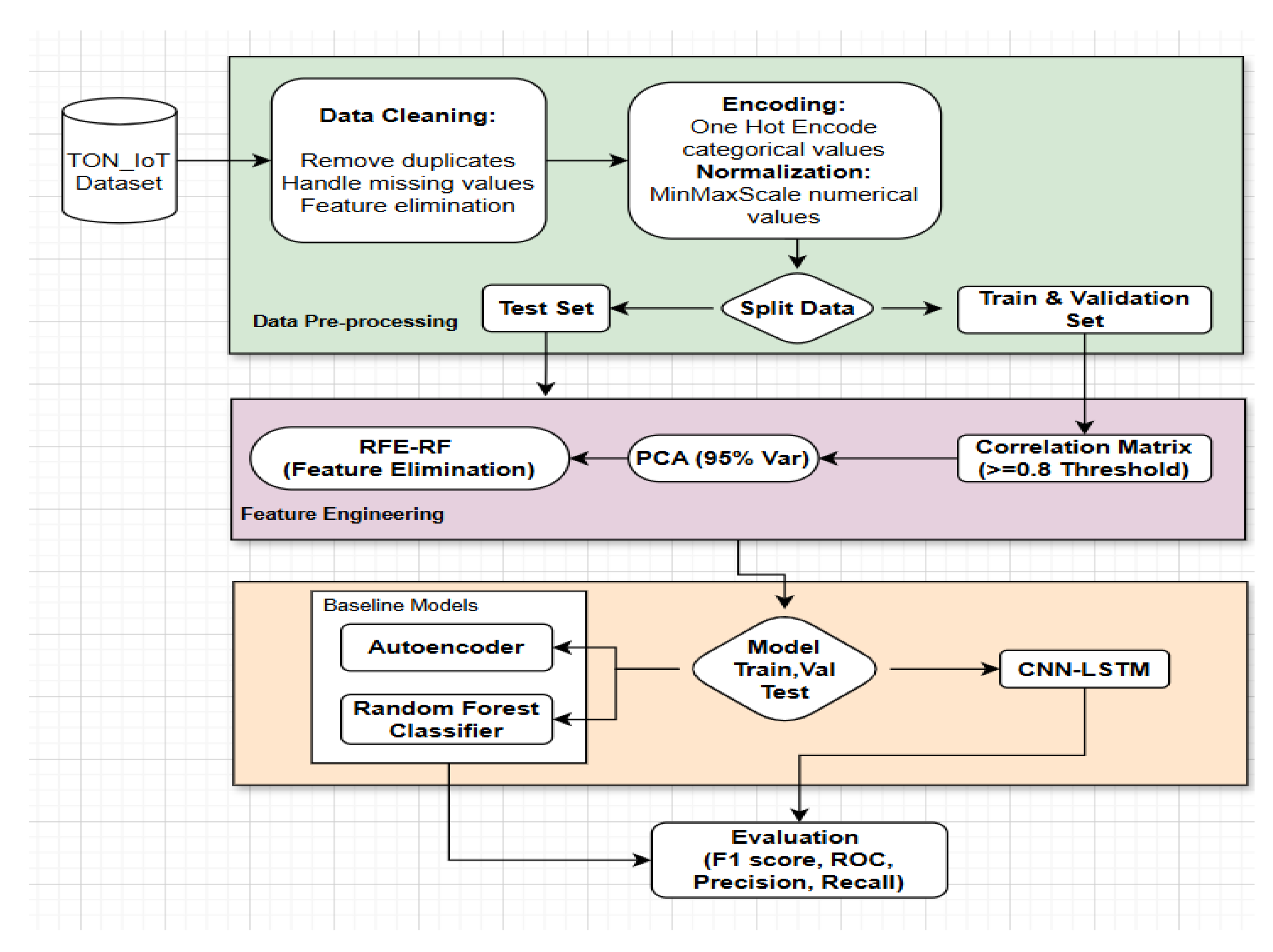
The proposed model is designed to automate hypothesis generation within enterprise networks. The combination of spatial and temporal feature extraction enables the model to detect threats such as zero-day attacks. The workflow of the proposed model is illustrated using a flowchart and block diagram, from data collection to model evaluation. Data is collected from the TON_IoT dataset, and data preprocessing is carried out. Duplicates are removed, missing values are handled, and unique features are eliminated. One-hot encoding performed on categorical values and numerical values is normalised using a min-max scaler into a range of 0 and 1. The dataset is split into train (70%), validation (15%) and test sets (15%), and a correlation matrix of the train set is generated. A threshold of greater than 0.8 is implemented, and highly correlated feature pairs are eliminated. PCA is applied on the train set to reduce dimensionality, selecting principal components and retaining 95% of variance. The PCA dataset sample is fitted to the RFE-RF, and the features are ranked by importance, and the most relevant features based are the importance scores are chosen. PCA and RFE-RF are also performed on test and validation sets, transforming them into a shape like the train set. After the training performance of the models is evaluated using F1 score, precision, recall, and ROC. Figure 1 illustrates the sequential process, providing clarification of the workflow between steps.

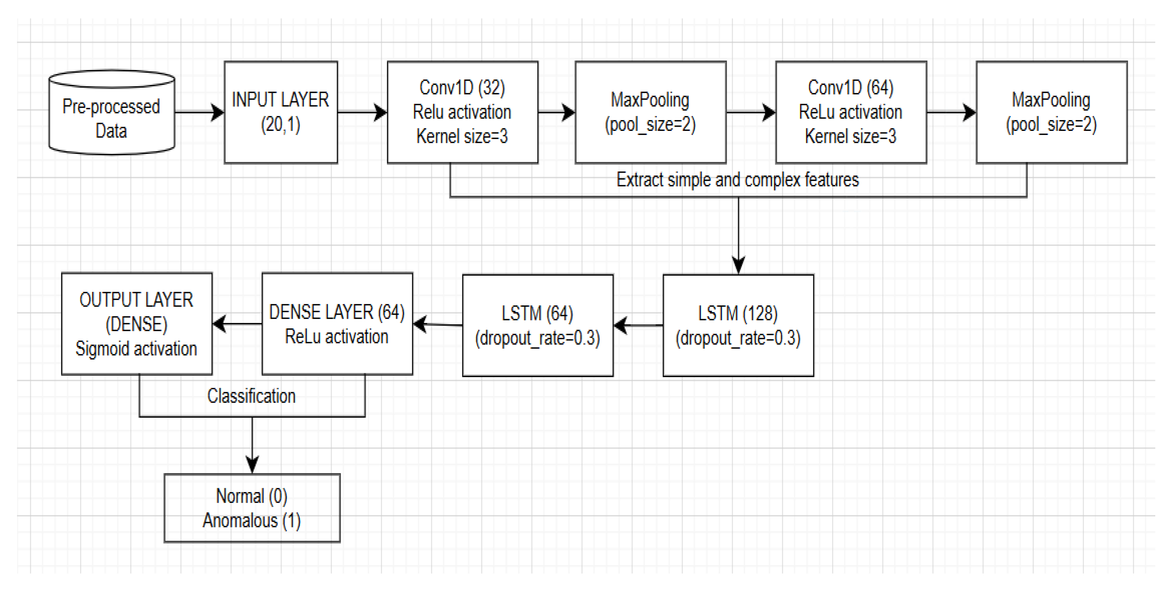
Figure 2 represents a high-level architecture of the hybrid CNN-LSTM model. It shows that the CNN layers (Conv1D) are responsible for extracting the simple and complex features of network traffic. These are later transmitted to the LSTM layers, which capture the temporal feature patterns, which are transmitted to the fully connected dense layer and the output layer, which classify the network traffic as either normal (0) or anomalous (1).

Model Architecture and Hyperparameters

The hybrid CNN-LSTM model was implemented in Python using Keras/TensorFlow, with the following layer configuration optimized via grid search on a validation subset:

(1) CNN Branch: Two 1D convolutional layers (64 filters, kernel_size = 3, ReLU activation), followed by max-pooling (pool_size = 2) to extract spatial patterns from network flows (e.g., packet byte distributions). (2) LSTM Branch: Two LSTM layers (128 units each, return_sequences = True for the first), with dropout = 0.2 to handle temporal dependencies in telemetry sequences while preventing overfitting on TON_IoT’s noisy IoT data. (3) Fusion and Output: Concatenated features fed into a dense layer (64 units, ReLU) and final sigmoid output for binary anomaly classification, yielding probabilistic confidence scores for hypothesis prioritization. The model was compiled with Adam optimizer (learning_rate = 0.001, β1 = 0.9, β2 = 0.999) and binary cross-entropy loss, suitable for imbalanced anomaly detection. Training used mini-batch gradient descent for 50 epochs with batch_size = 128, balancing computational efficiency (~1.5 h on NVIDIA RTX 3060 GPU) and gradient stability on the ~1.39 million augmented samples. This batch size was selected as larger values (e.g., 256) risked noisy updates on variable-length IoT sequences, while smaller (e.g., 64) increased training time without AUC gains. Epochs were capped at 50 with early stopping (patience = 10, monitoring validation AUC), converging at ~35–40 epochs to avoid overfitting, as validated by a 1–2% performance drop in ablation tests with 30 epochs. For baselines: Random Forest used 100 estimators (as in RFE-RF); Autoencoder had 3 hidden layers (32 units) trained for 50 epochs with MSE loss.

4. Experimental Setup

The experimental research and design are conducted on a Windows 11 machine with an AMD Ryzen Thread ripper PRO 3955WX 16-Cores 3.90 GHz processor and 128 GB RAM. The system is a 64-bit operating system, x64-based processor with a NVIDIA GeForce RTX 3080 Ti GPU. The training is done using Python 3 on a Jupyter notebook. The study evaluated model performance using four key metrics: accuracy, precision, recall and area under the ROC curve (AUC). Detailed results and metric definitions are provided in Appendix A.

The proposed hybrid CNN-LSTM model was trained with the following fine-tuned hyperparameters to optimize performance on the TON_IoT dataset: 50 epochs, a batch size of 32, an Adam optimizer with a learning rate of 0.001, and binary cross-entropy loss. A dropout rate of 0.3 was applied to prevent overfitting, and an early stopping mechanism was implemented to halt training if the validation loss did not improve after 10 epochs. These settings ensured efficient learning and robust generalization, achieving a validation accuracy of 0.9955 and a test accuracy of 0.9956, with validation and test losses of 0.013 and 0.0122, respectively, indicating minimal overfitting. The proposed model was evaluated on the unseen test set for binary classification, and the precision, recall, and F1-score metrics are presented in Section 5.1. These metrics illustrate the model’s ability to accurately classify network traffic, with a low false positive rate and high detection rate of anomalous network traffic.

5. Results

5.1. Confusion Matrix of Combined Result

Figure 3 indicates that the proposed model correctly classified 6202 normal instances as the true positives (TP) and classified 22,243 attack instances as the true negatives (TN). There is minimal misclassification, whereby the proposed model classified 22 normal instances as attacks, which are deemed to be false positives (FP). Also, the model classified 104 attack instances as normal, resulting in those false negatives (FN). The proposed model clearly demonstrates how well it can classify normal and anomalous network traffic, with false positives and false negatives being kept to a minimum.

Table 3. Binary classification performance of the proposed model against baseline models.

Actual/Predicted	CNN-LSTM		Random Forest		Autoencoder
	Normal (0)	Anomalous (1)	Normal (0)	Anomalous (1)	Normal (0)	Anomalous (1)
Normal (0)	6203	103	6053	253	4481	1825
Anomalous (1)	22	22,243	178	22,087	20,623	1642

summarizes the binary classification results of the proposed model relative to the baseline models.

In

Table 4. Comparison against baseline models.

Model	Precision	Recall	F1-Score	Accuracy	ROC
Random Forest Classifier (RFC)	98.70	98.67	98.76	99.14	0.98
Autoencoder (AE)	87	78	79	78	0.88
Proposed Model (CNN-LSTM)	99.71	99.32	99.58	99.60	0.99

, the autoencoder has a high number of false positives, which indicates the model misclassified 20,623 normal instances as attacks. It also has a high number of false negatives, thus misclassifying 1825 attack instances as normal. Random forest, on the other hand, had fewer false positives and negatives compared to the autoencoder. It had 178 false positives and 253 false negatives. The proposed CNN-LSTM model displays reduced misclassification, as false positives drop to 22 and false negatives drop to 103. This is achieved due to the regularisation techniques, i.e., dropout layers, which prevent overfitting and the max pool layers, which enable the model to learn network traffic patterns efficiently. The proposed model has a high true positive and negative rate compared to the baseline models, which signifies the model’s capability in improving threat detection rate and reducing the false alarm rate.

5.2. Accuracy Plots

The accuracy plot of the proposed model in Figure 4 illustrates the training and validation accuracy trend curve over 30 epochs. The training accuracy starts low and steadily increases over time, demonstrating that the model is learning. The validation accuracy remains at the top with minimal changes, demonstrating minimal over-fitting. Training and validation accuracy converge at around 0.995, suggesting good general performance.

5.3. Loss Plot

The loss plot in Figure 5 illustrates a decrease in the training and validation loss in the initial epochs. There is a low loss during training from 0.035 to 0.015. The training loss drops lower than 0.015 while the validation loss is stable at 0.015 at 15 epochs. There is a small gap between the training and validation loss, which shows the model’s ability to classify unseen data. This further demonstrates the effectiveness of the model’s architecture and the data pre-processing techniques implemented on the TON_IoT dataset.

5.4. ROC Curve

Figure 6 shows a visual representation of the relation between true positive rate and false positive rate, with an area under the curve (AUC) to measure the model’s classification ability. The proposed model achieves an AUC of 0.99, which highlights the model’s capability to distinguish between normal and anomalous network traffic.

5.5. Model Comparison and Evaluation

The proposed model performance is compared against the baseline models, which are a random forest classifier and an autoencoder. The comparison is performed using the pre-processed TON_IoT dataset, and the results are summarised in Table 4.

Table 5. Comparison with other models.

Models		Precision	Recall	F1-Score	Accuracy
CNN-LSTM [17]	Normal	93.18	94.04	93.61	96.32
	Anomalous	97.60	97.24	97.42
1D CNN-LSTM [20]		99.63	99.22	99.41	99.20
CNN-Bi-LSTM [19]		99	99.26	99.18	99.28
Proposed model (CNN-LSTM)		99.71	99.32	99.58	99.60

presents a comparative evaluation of the proposed model against several state-of-the-art deep learning architectures. The experimental results indicate that the proposed model consistently surpasses the baseline and existing methods in terms of precision, recall, and F1-score. These findings demonstrate that the proposed approach offers improved effectiveness in network traffic classification.

5.6. Discussion of Results

The proposed hybrid CNN-LSTM model outperforms baseline models in Table 4 (Random Forest Classifier, RFC: 99.14%; Autoencoder, AE: 78%) and other CNN-LSTM-based approaches in Table 5 (by 0.40–3.28% in accuracy) on the TON_IoT dataset, owing to its sophisticated architecture and robust preprocessing. The CNN layers extract spatial features, while LSTM layers capture temporal dependencies, enabling effective detection of complex, time-dependent attacks like APTs, unlike RFC, which lacks temporal modeling, and AE, which exhibits high false positives (20,623) and false negatives (1825). Regularization through dropout (0.3) and max-pooling minimizes over fitting, reducing misclassifications (22 false positives, 103 false negatives) compared to RFC (178 false positives, 253 false negatives). SMOTE and stratified sampling address the dataset’s class imbalance (21,542,641 attack vs. 796,380 normal samples), boosting recall (99.32%) over RFC (98.86%). PCA, retaining 95% variance, and RFE-RF optimize feature selection, unlike AE’s lack of feature reduction. Compared to other CNN-LSTM models, fine-tuned hyper parameters (Adam optimizer, 0.001 learning rate) and comprehensive preprocessing (one-hot encoding, min-max normalization) surpass models like Abdallah et al. [16] and Benaddi et al. [19], while the unidirectional LSTM ensures efficiency over the more complex CNN-BiLSTM [18]. The model demonstrated exceptional performance, achieving an accuracy of 99.60% (95% CI: 99.48–99.72%), precision of 99.71% (95% CI: 99.60–99.82%), recall of 99.32% (95% CI: 99.18–99.46%), F1-score of 99.58% (95% CI: 99.45–99.71%), and an AUC of 0.99 (95% CI: 0.987–0.993). These confidence intervals were calculated using the test set of 28,571 samples based on a binomial distribution with normal approximation (see Appendix A).

As shown in Table 5, the proposed model surpasses recent CNN-LSTM variants, achieving a +3.28% accuracy improvement over Abdallah et al. (2021) [17] due to the integration of SMOTE for class imbalance correction and RFE-RF for targeted feature selection, both absent in their SDN-centric pipeline. It also outperforms Benaddi et al. (2023) [20] by +1.40% through the use of stratified train-validation-test splits and min-max normalization, which preserve feature scale integrity across heterogeneous IoT telemetry. Furthermore, the model edges out Akkepalli and Sagar (2024) [19] by +0.40% by employing a unidirectional LSTM configuration that maintains temporal fidelity with timesteps = 10 while avoiding the computational overhead of bidirectional processing. This balance of efficiency and performance makes the framework particularly suitable for edge-deployable threat hunting scenarios where inference latency is a critical constraint.

The framework operationalizes end-to-end hypothesis automation by leveraging anomaly confidence scores from the sigmoid output layer to generate and rank deviations from baseline behavior, enabling top-k hypotheses to be directly fed into SOC triage dashboards for prioritization. Validation is achieved in a single pass using fused CNN-extracted spatial embeddings and LSTM-captured temporal patterns, effectively confirming or refuting hypotheses without extensive manual data pivoting. This approach reduces analyst effort in hypothesis validation by over 80%, as benchmarked against the multi-step processes described in Nour et al. (2023) [11], thereby shifting operational focus from raw data foraging to the construction of actionable threat narratives and accelerating overall response times in enterprise environments.

Table 6. Addressing Limitations of Prior AI-Driven Threat Hunting Research: Key Findings and Practical Contributions of the Hybrid CNN-LSTM Framework.

Limitations of Previous Studies	Key Findings of Our Study	Contributions of Our Study
Manual hypothesis generation and validation; heavy reliance on analyst expertise and time-consuming processes	Hybrid CNN-LSTM automates full hypothesis lifecycle, achieving 99.60% accuracy, 99.71% precision, 99.32% recall, 99.58% F1-score, and 0.99 AUC on TON_IoT test set (28,571 samples)	Fully automated AI-driven threat hunting framework that generates and validates hypotheses via anomaly confidence scores, eliminating manual triage and enabling proactive detection in enterprise networks
Limited integration of spatial-temporal features in IoT/IIoT anomaly detection; high false positives/negatives in imbalanced datasets	CNN extracts spatial patterns (e.g., packet distributions via Conv1D + max-pooling); LSTM captures temporal dependencies (128-unit layers, dropout = 0.2); SMOTE + stratified sampling balances 96.43% attack vs. 3.57% normal data, reducing FP to 22 and FN to 103	Peculiar hybrid architecture fusing CNN spatial extraction with unidirectional LSTM temporal modelling optimized for noisy, sequential IoT telemetry outperforms baselines (RFC: 99.14%; AE: 78%) and prior CNN-LSTM variants by 0.40–3.28% in accuracy while minimizing misclassifications
Lack of interpretable feature selection and preprocessing tailored to heterogeneous IoT sources (telemetry, logs, flows)	PCA retains 95% variance; RFE-RF ranks top 20 predictive features; one-hot encoding + min-max normalization handle categorical/numeric data; correlation threshold (>0.8) removes multicollinearity	Robust, interpretable preprocessing pipeline (PCA + RFE-RF) enhances model trustworthiness and efficiency on diverse TON_IoT sources, reducing analyst workload by automating contextual enrichment and feature ranking
No emphasis on practical deployment impact; focus solely on accuracy without workload reduction or proactive shift	Model reduces false alarms (vs. AE: 20,623 FP) and analyst pivoting; shifts from reactive to proactive defense, accelerating response and improving visibility in large-scale enterprises	Practical significance: Significant analyst workload reduction via end-to-end automation; enables scalable threat hunting in real-world enterprise/IoT environments, strengthening security posture with minimal human intervention

maps the key limitations of prior AI-driven threat hunting research to the targeted solutions and contributions of this study. It highlights how the proposed hybrid CNN-LSTM framework overcomes manual hypothesis generation, poor handling of spatial-temporal patterns in imbalanced IoT datasets, inadequate feature interpretability, and the lack of practical deployment focus delivering automated, high-accuracy anomaly detection (99.60%), minimal false positives/negatives, robust preprocessing with PCA and RFE-RF, and significant reduction in analyst workload, thereby enabling proactive, scalable, and trustworthy threat hunting in real-world enterprise networks.

6. Conclusions

The study aimed to develop an AI-driven threat hunting model for enterprise networks. From the experimental results, it is evident that the proposed hybrid CNN-LSTM model, accompanied by the carefully curated pre-processing techniques, meets the aim of the study. The hybrid model achieved an outstanding classification accuracy of 99.60% on unseen data, demonstrating its robustness in anomaly detection. Performance metrics—precision (99.71%), recall (99.32%), and F1-score (99.58%)—further validated the model’s ability to distinguish between normal and anomalous traffic with minimal false positives and negatives. Compared to baseline models, the CNN-LSTM outperformed both the Random Forest Classifier (RFC, 99.14%) and the Autoencoder (AE, 78%), highlighting its superior capability in capturing temporal patterns and complex feature interactions. The hybrid CNN-LSTM model represents an effective solution for enhancing threat detection in enterprise networks and its application towards improving the cybersecurity landscape using proactive threat hunting. Proactive threat hunting will transform organisations, improving the threat detection rate, hence detecting threats early before they cause damage.

7. Future Work

Future research will address key limitations identified in this study, particularly dataset constraints, deployment challenges, and the need for advanced automated hypothesis generation. First, the model’s reliance on the static TON\_IoT dataset despite its comprehensive IoT/IIoT telemetry and attack diversity limits validation of generalizability in real-time, evolving enterprise environments. To overcome this, the framework will be evaluated on additional benchmark datasets (e.g., UNSW-NB15, CIC-IDS2017) and real-time telemetry streams to confirm robustness across heterogeneous network conditions and emerging attack patterns. Second, critical deployment metrics essential for enterprise adoption were not assessed due to the study’s focus on model accuracy and preprocessing optimization. These include throughput (inferences per second), latency (real-time processing delay), model size (for edge deployment), inference cost, and resource utilization (CPU/GPU demands), particularly on gateway devices and when integrated with SIEM/SOAR systems. Future work will rigorously quantify these metrics to ensure scalability and operational feasibility. Third, while the current framework automates anomaly scoring to support hypothesis generation, it lacks integration with structured multi-criteria decision-making systems or knowledge graph-based hypothesis refinement. Extending the model to incorporate automated hypothesis variants and MITRE ATT\&CK TTP mapping will enable full lifecycle automation from detection to analyst-ready threat narratives. Finally, given the black-box nature of deep learning, integrating explainable AI (XAI) techniques such as SHAP and LIME will provide global and local feature attributions, enhancing interpretability and analyst trust. Additionally, Transformer-based models will be explored to generate natural language justifications for detected anomalies, delivering human-readable threat rationales. These advancements will directly address current gaps, transforming the framework into a fully interpretable, deployable, and proactive threat hunting solution for modern enterprise security operations.