Abstract
Fused deposition modeling (FDM), a method of additive manufacturing (AM), comprises the extrusion of materials via a nozzle and the subsequent combining of the layers to create 3D-printed objects. FDM is a widely used method for 3D-printing objects since it is affordable, effective, and easy to use. Some defects such as poor infill, elephant foot, layer shift, and poor surface finish arise in the FDM components at the printing stage due to variations in printing parameters such as printing speed, change in nozzle, or bed temperature. Proper fault classification is required to identify the cause of faulty products. In this work, the multi-sensory data are gathered using different sensors such as vibration, current, temperature, and sound sensors. The data acquisition is performed by using the National Instrumentation (NI) Data Acquisition System (DAQ) which provides the synchronous multi-sensory data for the model training. To induce the faults, the data are captured under different conditions such as variations in printing speed, temperate, and jerk during the printing. The collected data are used to train the machine learning (ML) and deep learning (DL) classification models to classify the variation in printing parameters. The ML models such as k-nearest neighbor (KNN), decision tree (DT), extra trees (ET), and random forest (RF) with convolutional neural network (CNN) as a DL model are used to classify the variable operation printing parameters. Out of the available models, in ML models, the RF classifier shows a classification accuracy of around 91% whereas, in the DL model, the CNN model shows good classification performance with accuracy ranging from 92 to 94% under variable operating conditions.
1. Introduction
Additive manufacturing (AM) is reigning in an Industrial Revolution 4.0 with its immense potential to change the face of industrial and global production via digitally robust and efficient engineering [1]. The predicted growth of the global AM market is expected to increase from USD 17.5 billion in 2024 to USD 37.4 billion by 2029, with a Compound Annual Growth Rate (CAGR) of 16.4% during the forecast period [2]. The 3D-printed components are manufactured by fusing the material in layer-by-layer form rather than being machined by forming the molds. Three-dimensional printing is preferable in components with complex internal channels or components having inside lattice or honeycomb architecture to save weight. Because there is no specialized molding equipment required, AM makes it possible to personalize a component by changing the specifications at the very last second. In addition, it has the potential to reduce a significant amount of assembly labor. This is due to the possibility of employing AM to build a component that would typically be made up of a number of smaller pieces as a single piece [3]. The process of AM is used by a number of companies in order to produce essential components for jet engine parts, as well as other aircraft parts, medical equipment, and surgical implants [4]. Although it is still in its infancy as a production option, its user base and application base are expanding. Machines for AM will develop quicker, have larger built envelopes, and have a better understanding of how to process different materials. A part that can be effectively manufactured today is probably still going to be machined tomorrow. However, machining will ultimately give way to AM for certain components. However, it is advisable to consider additive as a complementing concept. The invention of Stereolithography (SLA) by Chuck Hull in 1987, which uses a laser to solidify small layers of ultraviolet (UV) light-sensitive liquid polymer, marked the beginning of AM. With AM, it may be feasible to produce intricate and customized items quickly, with fewer experienced employees, shorter product life cycles, and quicker delivery. AM is utilized to create a variety of goods in an increasing number of sectors, including aerospace, automotive, and medical sectors [5]. Each industry benefits from AM’s advantages, but the aerospace sector prioritizes AM due to its ability to produce intricate geometric element components for aircraft and its capacity to cut weight [5]. Similar to how AM may be used in the medical sector to make medical models, surgical implants, surgical guides, external guides, and bio-manufacturing, AM is frequently used in the automobile business to quickly prototype a range of materials [6]. AM is not just believed to replace conventional manufacturing due to the time consumed to manufacture the components; conventional manufacturing is still preferable for the simple and easy mode of production of components, but AM is the best choice for manufacturers in manufacturing light batches of complex designed components. With his, one could come to the point that AM is important for the manufacturing of light, complex designs that can be expensive and difficult to manufacture using traditional manufacturing techniques, like milling or any other machining technique [7].
AM provides a range of advantages for both production and prototyping. Selective laser sintering (SLS), SLA, FDM, and digital light processing (DLP) are examples of additive manufacturing (AM) methods [8]. As in FDM, for the type of AM, the thermoplastic filament is used by heating to a certain melting point, and then using an extruder, the melted filament is extracted in layers to create a necessary component in a three-dimensional object; the ease of use is much better than compared to other AM alternatives available, and FDM is used widely enough to produce intricate geometrical things at a minimal cost. In 3D-printed products, defects arise mainly in printed components due to inevitable changes in process parameters, for example, the variation in printing speed, bed leveling may be disrupted, the temperature of the nozzle or extruder temperature may vary, or there may be structural pliability [9]. It can be difficult to recognize errors that arise during the 3D-printing process [10]. In this case, a data capture and monitoring system are needed for efficient error diagnosis [11]. If defect product classification is implemented correctly, it can help us identify the root cause of the error. Here, material properties and printing process failure are the main causes of defects, and the majority of them are brought on by temperature and vibration changes during the printing stage. With many benefits come many drawbacks, including faults that must be checked during real-time execution, the size restriction of the component, anisotropic mechanical characteristics, the construction of overhang surfaces, and edge warping. Pillowing, poor adhesion, layer shifting, elephant foot, and infill gaps are issues that need further investigation and research [12]. To deploy this product with the utmost quality required is the detection of defects that occur in AM.
This work mainly focuses on the faults that occur in 3D printing due to variations in printing parameters such as printing speed, printing jerk, and printing temperature. The accurate classification of these variations in printing parameters helps to identify faults and the cause of faults in the product.
2. Related Work
Most of the low-cost FDM 3D printers lack functionality for process monitoring during the printing phase. In such cases, real-time data gathering and monitoring are made possible via an external data collection system and multiple sensors. Even the most sophisticated FDM machines cannot distinguish between regular and abnormal (faulty) data for analytics as they can only monitor data. The main causes of faults may also be found with the use of accurate data analytics. Thermocouple and fibre Bragg grating (FBG) sensors were used by Kousiatza et al. to evaluate real-time field parameters and their impact on multilayer deposition to identify anomalies [13]. In the AM process, the data-driven, predictive method is used to improve the final product’s surface quality [14]. Multiple sensors, such as an accelerometer, thermocouples, and infrared temperature sensors, were used to gather real-time data such as temperature and vibrations [15]. Using sensor data, physical system process characteristics may be tracked in cyberspace throughout each communication network clock cycle. The many deployed sensor components on the physical system are capable of measuring a wide range of process parameters, including temperature, humidity, magnetic, vibration, and current. Using real-time sensor data to predict the behavior of the physical system properly, the anomaly may recognize and represent a physical system in the actual world [16]. Proper defect identification is a crucial component in producing high-quality items using AM. The issues may be identified by utilizing data-driven techniques [17].
2.1. Monitoring the AM Process
Convolutional and deep neural networks are used in AM methods to automatically monitor the end product’s quality. If the layer-by-layer deposition process is recorded and analyzed in real time, internal and surface faults of the completed product created by 3D printing may be assessed and classified into several categories [18]. When huge products are created using an FDM-based 3D printer, the bulk of flaws that come from the rumpled product occur in the spaces between the layers of the printing process. Time and resources are wasted as a consequence of this. Langeland et al. used two cameras positioned at various angles to capture real-time images of material deposition. On the basis of the material’s surface, a DL model was developed using them to predict flaws [19]. One of the most challenging problems in AM is maintaining the quality of the 3D result. On the other hand, image processing and supervised ML models make it possible to accurately forecast if a 3D object has flaws. The datasets are divided into categories for abnormal and normal picture datasets using machine models as the framework. Researchers Delli et al. conducted research employing materials consisting of Acrylonitrile Butadiene Styrene (ABS) and Polylactic Acid (PLA), and they made predictions about the types of component geometry flaws that would be added to the finished products based on the surface finishing of the materials [20,21].
2.2. Data-Driven Classification Model
In the data-driven model, from raw data, significant features are extracted (signals) to obtain valuable information, where data are received via sensors from machines or devices carrying out certain tasks designated for defect classification. The data are analyzed using various machine learning classifier techniques, such as ET classifiers, DT classifiers, RF classifiers, and KNN classifiers. Data-driven models rely heavily on proper sensor placement; if the sensors are not in the right places, the data collecting system may have trouble gathering reliable data, leading to unreliable model predictions. This study’s main objective is to examine the data-driven approach for categorizing defects in the final FDM 3D-printed component. For different processes and applications, a variety of ML and DL models have been researched to identify the defects in manufacturing [22,23]. Day et al. provided a thorough explanation of all the ML approaches and various algorithms with their structures and an understanding of how ML may provide a wide variety of algorithms for fault detection [24]. A large amount of research has been conducted on ML architectures in conjunction with acoustical or visual monitoring to identify errors automatically during 3D printing. The position of the sensors is given priority in many studies that utilize monitoring based on sensors because it significantly affects the finished printed product [25]. Table 1 provides the available literature related to fault classification in the field of additive manufacturing.

Table 1.
Literature review of fault classification in the AM process.
3. Methodology
In this work, the real-time data are collected from the 3D printer using different sensors such as vibration, temperature, sound, and current. The raw data are collected under variable operating conditions by varying the temperature, speed, and jerk during the 3D printing. The collected raw data are pre-processed and provided to the different classification models for the fault classification. Figure 1 shows the overall methodology of the work. The details of each phase of the methodology are discussed in the following sub-sections.
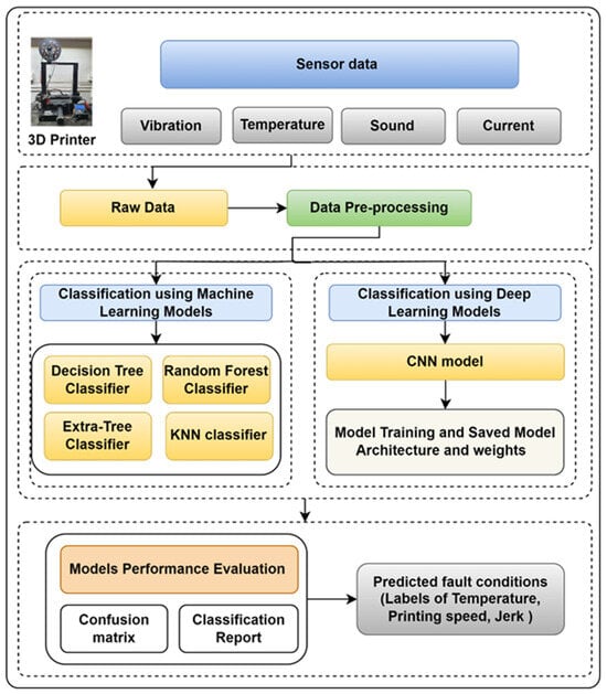
Figure 1.
The overall methodology of fault detection in 3D-printed products.
The data collection is carried out with the help of the Data Acquisition (DAQ) instrument; the signal is amplified and converted using analog-to-digital converters, and digital-to-analog converters in the later stage. This proposed system receives input signals from vibration, current, temperature, and sound sensors. Collected data are recorded in a Comma-Separated Values (CSV) format with a 1 kHz sampling rate. The captured data are then provided to the ML and DL models.
3.1. Experimentation and Data Acquisition
The sensors are mounted on the Ender-3, 3D printer manufactured by Creality located at Shenzhen, China. The detailed specifications of the printer are given in Table 2.

Table 2.
Description of 3D printer used for experimentation.
The mounted sensors are connected with the DAQ system manufactured by the National Instruments (NI) Corporation which is a prominent American company located in Austin, Texas. The DAQ’s analog input terminals and analyzed using the DAQExpress software (5.1). A detailed description of DAQ is given in Table 3.

Table 3.
Description of National Instrument DAQ 612 system.
The various types of sensors used are vibration, sound, temperature, and current. Figure 2 and Figure 3 show the overall setup of the data collection from the 3D printer and sensor locations on the 3D printer, respectively. The vibration sensor that has been used here is VBR series—VBR1D03A manufactured by Microdetector company based in Modena, Italy which tracks down the vibrations in a 3-axis inclination. The PT-100 temperature sensor, manufactured by Omega Engineering company located in the USA is used. It is a specialized kind of sensor that belongs to a category known as Resistance Temperature Detectors (RTDs). The sound sensor used is an LM393 sound detection sensor, and the current sensor, the Pico TA301 Current Clamp manufactured by Pico Technology Company located in Cambridgeshire, United Kingdom, is used to measure the incoming current to a 3D printer.
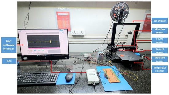
Figure 2.
Experimental setup for data collection.
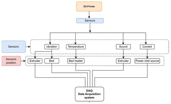
Figure 3.
Sensor mounting position and Data Acquisition System (DAQ).
In this work, a basic cubical shape component is created using a 3D printer under ideal circumstances. The Ultimaker Cura software (5.8) is used to generate the G-codes for 3D printing from the CAD model. Ultimaker Cura is one of the most popular and widely used slicing software in the 3D-printing community. Developed by Ultimaker, a leading manufacturer of 3D printers, it is open-source software that converts 3D models into printable G-code instructions for 3D printers. The Polylactic Acid (PLA) material is used for printing purposes. This material is cost effective and user friendly for 3D-printed products. The normal printing parameters of the PLA material are specified in Table 4.

Table 4.
Generalized specification of PLA material used in FDM 3D printers.
Several sensors are used to capture real-time data. Vibration, sound, and current sensors are used in this work for data collection purposes. Various fault conditions and their interrelated effect were efficiently captured in the multi-sensory data. It is simple to identify structural defects in the FDM since the vibration sensor was efficiently capable of capturing variations in vibration intensity throughout the printing stage. The current sensor and sound sensor make it easy to assess the health of a 3D printer. The current sensor measures the variations in the input power supply. The sound sensor records the noise made by each of the machine’s separate motors. The fluctuation in current drawn and the associated noise produced by each individual motor occurs during the moment of the machine’s introduction of fault circumstances. With the aid of sensors and the DAQ graphical user interface, the data are gathered and exported in CSV format. The data contain multiple input sensory data such as vibration, sound, current, and temperature; these parameters are selected, the data have been collected with a desired sample frequency of 1kHz for each sample created in FDM, and each sample’s sensory data have been recorded with different parameter variations.
The variations have been added according to the case sheet that has been created shown in Table 5. It shows variable operating parameters and their ranges considered during the data collection. The case sheet has been created by considering multiple elements that affect the FDM process due to various factors that come into consideration in the FDM process, the multiple elements that affect the FDM process are motor and driver temperature, jerk, bed leveling, and printing speed.

Table 5.
Variable operating parameters and their ranges.
These are the various factors that have been identified as key factors that affect the FDM process. The printing time varies from 5 min to 20 min for a single sample, the data contain an approx. range from 3 lacs to 15 lacs data entries of all the sensors based on the time variations according to the data collection conditions. In the variable jerk condition, a total of ten runs were taken from 10 to 500 m/s3 with a step size of 50 m/s3. In variable speed conditions, a total of 28 runs were taken from 40 to 310 mm/sec with a step size of 10mm/sec. The collected data are through the NI DAQ 612 which already has the data synchronization capability and has filtering options. Along with that, the data scaling is performed on the data to normalize the data using a min–max scaler which scales the multi-sensors data in the range of 0–1 unit. The time series features are extracted from the raw data to obtain more insights from the incoming data. Further, to avoid the overfitting of the model during the training–testing phase, the callback functions are created which prevent the model’s overfitting by applying the early stopping during the training phase of the model by finding the optimized value of epochs. Figure 4 shows the collected ten minutes of mean values of normalized vibration, current, temperature, and sound sensor signal representation for different operating conditions.
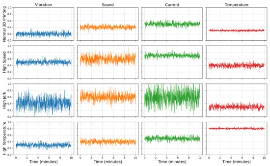
Figure 4.
Collected normalized vibration, current, temperature, and sound sensor signal representation for different operating conditions.
Table 6 shows the effect of variable operating 3D-printing parameters on the final printed products. The PLA material is used for printing purposes. This material is cost effective and user friendly for 3D-printed products. The classification of the print is based on visual impression. Initially, the product is printed at the normal printing parameters and printed products are considered as the normal print, whereas to generate the faulty printed products, the printing parameters are varied manually to induce the faults in the printed product. Due to the high printing speed, different faults such as poor infill and elephant foot are developed in the end product. High-jerk conditions are responsible for the development of faults such as poor infilling with the layer shifting that takes place in the end product. Due to high extrusion or nozzle temperatures, the overheating material takes place which leads to poor surface finishing observed in the 3D-printed products.

Table 6.
Fault condition and fault labels with images.
3.2. Models Used for the Fault Classification
In this work, Python 3.8 programming language is used for building the ML and DL models. The Anaconda Jupyter Notebook is used for coding purposes. The ML models such as KNN, DT, ETC, and RFC are used to classify the different operating parameters of the 3D-printing products. In the DL model, the CNN model is used for classification purposes. The performance of different classification methods is evaluated for predicting the likelihood of an event occurring based on input parameters such as speed, jerk, and temperature. The evaluation is conducted under three different conditions, namely, temperature, jerk, and printing speed. Classification models are trained to assign input data to one of several predefined classes based on the patterns found in the input data. Overall, 80% of the data are used for training purposes whereas 20% of the data are used for the purpose of model testing. A classification model learns from labeled data, where the input data are associated with a known output or class label. The performance of a classification model can be evaluated based on several metrics, including precision, recall, F1- score, and accuracy. Precision is a measure of how often the model correctly identifies the positive class (i.e., the class we are interested in) among all the predicted positive classes. Recall, on the other hand, measures how often the model correctly identifies the positive class among all the true positive classes. F1-score is a weighted average of precision and recall, which considers both measures. Accuracy, the most used metric, measures the percentage of correct predictions among all the predictions.
Decision tree classification is a non-parametric supervised learning method used for classification tasks. It is a simple and interpretable model that works by recursively partitioning the input space into smaller and smaller subspaces, based on the value of the input features. The following are the best-tuned parameters found in the while hyperparameter tuning.
Extra-tree classification is a variant of decision trees that is more random and less computationally intensive. It works by randomly selecting a subset of features and a random threshold value for each feature at each node.
Random forest classification is an ensemble learning method that uses multiple decision trees to improve the accuracy and stability of the classification. It works by training multiple decision trees on random subsets of the input data and features and then aggregating their predictions. KNN classification, on the other hand, is a non-parametric method that classifies a new data point based on the class of the k-nearest neighbors in the training set.
Finally, 1D CNN classification is a deep learning method that uses convolutional layers to automatically learn relevant features from the input data. To build a neural network, the TensorFlow (TF) library is used. TF is an open-source library developed by Google for machine learning and deep learning. It provides tools for building and training neural networks. Table 7 shows the model architecture used for the one-dimensional CNN model.

Table 7.
1D CNN layers and parameters used for the model training.
The convolutional layers slide a set of filters over the input data and extract features based on the patterns found in the data. These features are then passed through fully connected layers that classify the input data. The models are trained using the early-stopping approach during the training phase. The early stopping method stops training when validation performance no longer improves, preventing overfitting.
The performance of the above models is evaluated based on the confusion matrix and the classification report. The confusion matrix indicates the number of true positive (TP), true negative (TN), false positive (FP), and false negative (FN) instances predicted for each class. The axis labels of the confusion matrix indicate the names or categories of classes classified during the classification. The x- and y-axis labels of the confusion matrix indicate the predicted and true classes which are to be classified.
4. Results and Discussion
The variable operating conditions are classified using the different ML and DL models. The Section 4 is divided into the different sub-sections such as the model classification accuracies for the variable speed, jerk, and temperature conditions. Different performance parameters such as precision, recall, F1-score, and accuracy are considered for classification model evolution.
4.1. Model Performance for the Variable Printing Temperature Conditions
In the ML models, the KNN, ETC, DTC, and RFC are used to check the model’s performance. Overall, 80% of the data are used for training purposes whereas 20% of the data are used for the purpose of model testing. Table 8 shows the shows performance of the different ML models. The accuracy of the ML models ranges from 0.73 to 0.90. The KNN provides an accuracy of up to 0.73, whereas DTC and ETC provide an accuracy of around 0.89. In ML models, RFC, which comes under the family of ensemble learning, gives the highest accuracy of 90%.

Table 8.
Different ML and DL model performances for the variable temperature in 3D printing.
Figure 5 shows the confusion matrix of the RFC model for variable temperature conditions. From the confusion matrix, it is observed that the model is effectively able to classify the different classes based on the variable operating printing temperature.
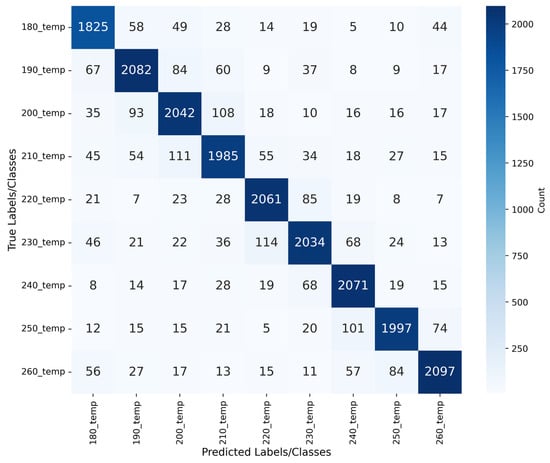
Figure 5.
RFC model confusion matrix for variable temperature condition.
In the DL models, 1D CNN is used for the classification. The temperature variation model’s learning curves demonstrate that it is also doing well on the training set of data. Figure 6 indicates that the model is becoming better by minimizing the misclassification errors between the predicted and actual temperature classes, and the loss curve is gradually declining. Likewise, the accuracy curve is constantly rising, showing that the model’s temperature predictions are improving.
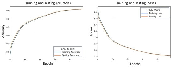
Figure 6.
CNN model learning curve for variable temperature conditions.
These findings imply that the temperature model performs well in forecasting temperature based on the input characteristics and can capture the patterns and correlations in the data. The data are up-sampled before passing to the CNN model. CNN provides a classification accuracy of 0.92%. Figure 7 shows the confusion matrix of the CNN model which indicates that the model is easily able to classify the variable printing temperature with the CNN model.
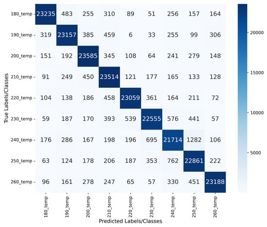
Figure 7.
CNN model confusion matrix for variable temperature condition.
4.2. Model Performance for the Variable Printing Speed Conditions
Similarly, to check the performance of classification models under variable printing speed conditions, different ML and DL models are used. Table 9 shows the performance of different classification models under variable printing speed conditions.

Table 9.
Different ML and DL models performances for the variable speed in 3D printing.
In ML models, the ETC shows better classification accuracy up to 0.92. Figure 8 shows the confusion matrix of the best-performing ML model, i.e., the ETC model’s performance for variable speed conditions. From the confusion matrix, it is observed that the model is effectively able to classify the different classes based on the variable operating printing speed.
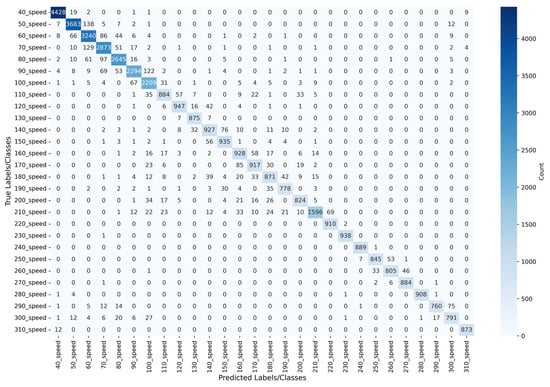
Figure 8.
ETC model confusion matrix for variable speed condition.
In the CNN model, for the variable speed condition, in Figure 9, learning curves demonstrate how well the model performed on the training set of data. The curve indicates that the model is becoming better by minimizing the misclassification errors between the anticipated and actual speed classes with the loss curve having a consistent downward trend. The accuracy curve is likewise constantly rising, suggesting that the model’s estimates of variable speed classification are improving. These findings imply that the speed model performs well at predicting speed based on input variables and can identify patterns and correlations in the data.
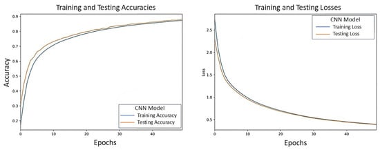
Figure 9.
CNN model learning curve for variable printing speed conditions.
The CNN model provides a classification accuracy of 93% for the variable printing speed conditions. The confusion matrix for the same is shown in Figure 10.
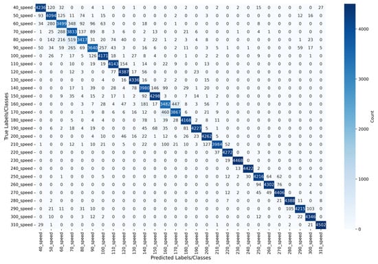
Figure 10.
CNN model confusion matrix of variable speed condition.
4.3. Model Performance for the Variable Printing Jerk Conditions
The ML and DL models are used to classify the 3D-printed products under variable printing jerk conditions. In ML models, the classification accuracy varies from 74% to 91%. The KNN model provides the lowest accuracy of 74%, while the RFC provides the classification accuracy of 91% due to its property of ensemble learning. Table 10 shows the accuracy, precision, recall, and F1-score of the different ML models under variable printing jerk conditions.

Table 10.
Different ML and DL model performances for the variable jerk in 3D printing.
Figure 11 shows the confusion matrix of the best-performing ML model, i.e., the RFR model’s performance for variable jerk conditions. From the confusion matrix, it is observed that the model is effectively able to classify the different classes based on the variable operating printing speed.

Figure 11.
RFC model confusion matrix for variable jerk condition.
In the DL category, the CNN model is used for the classification of variable jerk conditions during the 3D-printing process. The data are up-sampled before passing to the CNN model. Figure 12 represents the learning curves for the classification models using the Jerk method. Training and testing accuracy will be high with increasing the number of epochs and loss will be continuously decreasing.
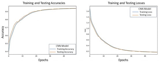
Figure 12.
CNN model Learning curve for variable Jerk conditions.
Likewise, the jerk model’s learning curves show strong performance on the training set of data. Indicating that the model is becoming better at minimizing errors between anticipated and real jerk levels, the loss curve is gradually declining. Likewise, the accuracy curve is constantly rising, suggesting that the model’s jerk predictions are growing more accurate.
These findings indicate that the jerk model performs well in jerk prediction based on input characteristics and can identify patterns and correlations in the data. Figure 13 shows the confusion matrix under variable jerk conditions during the 3D-printing process. From the confusion matrix, it is clear that the CNN model is able to classify the different jerk conditions with an accuracy of 94%.
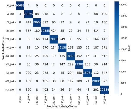
Figure 13.
CNN model confusion matrix of variable jerk conditions.
Table 11 shows the consolidated result based on the performance of the different models under variable printing parameters. The evaluation results showed that the CNN classification method outperformed all the other methods under all three conditions, achieving the highest precision, recall, F1-score, and accuracy. The results also showed that the decision tree, extra-tree, and random forest classification methods performed fairly well under different conditions, while the KNN method had the lowest performance. As KNN model classifies the data based on a simple distance (Euclidean or Manhattan)-based approach. KNN struggles with higher dimensional complex data. So, KNN shows moderate classification performance across all the variable printing parameters. TheET classifier performs very well, particularly for speed. Its tree-based nature allows it to capture non-linear relationships effectively. The DTC performs similarly to ETC but is slightly less robust overall. It maintains consistency across all metrics for the different variables, showcasing its ability to handle discrete splits.

Table 11.
Model performance for variation in temperatures, speed, and jerk.
Random forest shows excellent performance across all variables, with high precision, recall, and accuracy, especially for speed and jerk. Its ensemble approach, which reduces variance compared to a single decision tree, explains its superior performance. It is more stable and less prone to overfitting than the extra-tree classifier. CNN outperforms all other models, particularly for jerk data. Its deep learning architecture allows it to capture complex patterns and relationships that simpler models might miss. This performance suggests that CNN is highly effective for feature-rich data, making it ideal for scenarios where complex interactions between features are expected. These results highlight the importance of selecting the appropriate classification method for the specific task and data characteristics. The comparative study of different classification models provided valuable insights into the performance of different models for predicting the likelihood of an event occurring based on input parameters. The multi-sensory data with a high data-sampling-rate approach used in this work provides the high reliability of the incoming data which helps to build a trustworthy model for fault classification in 3D-printed products.
5. Conclusions
In this work, the various fault conditions are induced in fused deposition modeling at the printing stage, which results in a poor infill, elephant foot, layer shift, and poor surface finish in 3D-printed products. The multi-sensor data with variations according to the induced fault condition have been collected using DAQ that captures real-time signals of multiple sensors that are vibration, sound, temperature, and current. In this work, a a classification model is developed for predicting the likelihood of an event based on input parameters such as speed, jerk, and temperature. The collected data are used to train the ML and DL classification models to classify the changes in printing parameters. The ML models such as KNN, DT, ET, and RF with CNN as a DL model are used to classify the variable operation printing parameters. In ML models, the RF model gives the maximum classification accuracy of 90–91% for the variable operating conditions. In DL models, the CNN model provides the maximum accuracy of 92–94% for the different variable speed, jerk, and temperature conditions. The comparative study of different classification methods provided valuable insights into the performance of different models for predicting the likelihood of an event occurring based on input parameters. By evaluating the performance of different models under different conditions, it is observed that the CNN model performs well and is able to classify the faults effectively that occur due to variations in printing parameters.
Author Contributions
Conceptualization, S.K. and S.S.; methodology, S.S.; software, S.S.; validation, S.K. and A.B.; formal analysis, A.B.; resources, S.K.; data curation, S.S.; writing—original draft preparation, S.S.; writing—review and editing, S.S.; supervision, A.B.; project administration, S.K.; funding acquisition, S.K. and A.B. All authors have read and agreed to the published version of the manuscript.
Funding
This work was supported by the Research Support Fund (RSF) of Symbiosis International (Deemed University), Pune, India.
Institutional Review Board Statement
Not applicable.
Informed Consent Statement
Not applicable.
Data Availability Statement
The raw data supporting the conclusions of this article will be made available by the authors on request.
Conflicts of Interest
The authors declare no conflicts of interest.
References
- Bogue, R. 3D Printing: The Dawn of a New Era in Manufacturing? Assem. Autom. 2013, 33, 307–311. [Google Scholar] [CrossRef]
- MarketsandMarkets. 3D Printing Market. Available online: https://www.marketsandmarkets.com/Market-Reports/3d-printing-market-1276.html (accessed on 20 April 2024).
- Yan, X.; Bethers, B.; Chen, H.; Xiao, S.; Lin, S.; Tran, B.; Jiang, L.; Yang, Y. Recent Advancements in Biomimetic 3D Printing Materials with Enhanced Mechanical Properties. Front. Mater. 2021, 8, 735220. [Google Scholar] [CrossRef]
- Schiller, G.J. Additive Manufacturing for Aerospace. In Proceedings of the IEEE Aerospace Conference, Big Sky, MT, USA, 7–14 March 2015; pp. 1–8. [Google Scholar] [CrossRef]
- Wong, K.V.; Hernandez, A. A Review of Additive Manufacturing. ISRN Mech. Eng. 2012, 2012, 208760. [Google Scholar] [CrossRef]
- Rouf, S.; Malik, A.; Singh, N.; Raina, A.; Naveed, N.; Siddiqui, M.I.H.; Haq, M.I.U. Additive Manufacturing Technologies: Industrial and Medical Applications. Sustain. Oper. Comput. 2022, 3, 100107. [Google Scholar] [CrossRef]
- Sayyad, S.; Kumar, S.; Bongale, A.; Kamat, P.; Patil, S.; Kotecha, K. Data-Driven Remaining Useful Life Estimation for Milling Process: Sensors, Algorithms, Datasets, and Future Directions. IEEE Access 2021, 9, 110255–110286. [Google Scholar] [CrossRef]
- Gunaydin, K.; Türkmen, H. Common FDM 3D Printing Defects. In Proceedings of the International Congress on 3D Printing (Additive Manufacturing) Technologies and Digital Industry, Antalya, Turkey, 19–21 April 2018. [Google Scholar]
- Galati, M.; Minetola, P. On the Measure of the Aesthetic Quality of 3D Printed Plastic Parts. Int. J. Interact. Des. Manuf. 2019, 14, 381–392. [Google Scholar] [CrossRef]
- Carolo, L. Gaps in 3D Prints: How to Fix & Avoid Them. All3DP. 5 December 2023. Available online: https://all3dp.com/2/gaps-in-3d-print-top-layer-gaps-between-lines/ (accessed on 5 May 2024).
- Sampedro, G.A.R.; Agron, D.J.S.; Amaizu, G.C.; Kim, D.-S.; Lee, J.-M. Design of an In-Process Quality Monitoring Strategy for FDM-Type 3D Printer Using Deep Learning. Appl. Sci. 2022, 12, 8753. [Google Scholar] [CrossRef]
- Manufactur3D. Common Problems in 3D Printing & How to Resolve Them–Part I. Manufactur3D. 3 December 2018. Available online: https://manufactur3dmag.com/common-problems-in-3d-printing-how-to-resolve-them-part-i/ (accessed on 5 May 2024).
- Kousiatza, C.; Karalekas, D. In-Situ Monitoring of Strain and Temperature Distributions During the Fused Deposition Modeling Process. Mater. Des. 2016, 97, 400–406. [Google Scholar] [CrossRef]
- Sammaiah, P.; Rushmamanisha, K.; Praveenadevi, N.; Reddy, I.R. The influence of process parameters on the surface roughness of the 3d printed part in FDM process. IOP Conf. Ser. Mater. Sci. Eng. 2020, 981, 042021. [Google Scholar] [CrossRef]
- Rao, P.K.; Liu, J.; Roberson, D.; Kong, Z.; Williams, C. Online Real-Time Quality Monitoring in Additive Manufacturing Processes Using Heterogeneous Sensors. J. Manuf. Sci. Eng. 2015, 137, 061007. [Google Scholar] [CrossRef]
- Lee, J.; Bagheri, B.; Jin, C. Introduction to Cyber Manufacturing. Manuf. Lett. 2016, 8, 11–15. [Google Scholar] [CrossRef]
- Long, J.; Sun, Z.; Li, C.; Hong, Y.; Bai, Y.; Zhang, S. A novel sparse echo autoencoder network for data-driven fault diagnosis of delta 3-D printers. IEEE Trans. Instrum. Meas. 2019, 69, 683–692. [Google Scholar] [CrossRef]
- Banadaki, Y.; Razaviarab, N.; Fekrmandi, H.; Sharifi, S. Toward Enabling a Reliable Quality Monitoring System for Additive Manufacturing Process Using Deep Convolutional Neural Networks. arXiv 2020, arXiv:2003.08749. [Google Scholar]
- Zhang, Z.; Fidan, I.; Allen, M. Detection of Material Extrusion In-Process Failures via Deep Learning. Inventions 2020, 5, 25. [Google Scholar] [CrossRef]
- Langeland, S.A. Automatic Error Detection in 3D Printing Using Computer Vision. Master’s Thesis, The University of Bergen, Bergen, Norway, 2020. Available online: https://bora.uib.no/bora-xmlui/handle/1956/22384 (accessed on 15 May 2024).
- Stoyanov, S.; Bailey, C. Machine Learning for Additive Manufacturing of Electronics. In Proceedings of the 2017 40th International Spring Seminar on Electronics Technology (ISSE), Sofia, Bulgaria, 10–14 May 2017. [Google Scholar]
- Misal, A.; Karandikar, H.; Sayyad, S.; Bongale, A.; Kumar, S.; Warke, V. Milling Tool Wear Estimation Using Machine Learning with Feature Extraction Approach. In Proceedings of the 2024 MIT Art, Design and Technology School of Computing International Conference (MITADTSoCiCon), Pune, India, 25–27 April 2024; pp. 1–7. [Google Scholar] [CrossRef]
- Wan, J.; Canedo, A.; Al Faruque, M.A. Cyber–Physical Codesign at the Functional Level for Multidomain Automotive Systems. IEEE Syst. J. 2015, 11, 2949–2959. [Google Scholar] [CrossRef]
- Dey, A. Machine Learning Algorithms: A Review. Int. J. Comput. Sci. Inf. Technol. 2016, 7, 1174–1179. [Google Scholar]
- Westphal, E.; Seitz, H. Machine learning for the intelligent analysis of 3D printing conditions using environmental sensor data to support quality assurance. Addit. Manuf. 2022, 50, 102535. [Google Scholar] [CrossRef]
- Li, Z.; Zhang, Z.; Shi, J.; Wu, D. Prediction of Surface Roughness in Extrusion-Based Additive Manufacturing with Machine Learning. Robot. Comput. Manuf. 2019, 57, 488–495. [Google Scholar] [CrossRef]
- Zhang, R.; Liu, J.; Li, M.; Wang, X. Real-Time Monitoring of Fused Deposition Modeling Using Thermal Imaging and Deep Learning. J. Manuf. Process. 2020, 54, 276–283. [Google Scholar] [CrossRef]
- Kim, J.S.; Lee, C.S.; Kim, S.M.; Lee, S.W. Development of Data-Driven In-Situ Monitoring and Diagnosis System of Fused Deposition Modeling (FDM) Process Based on Support Vector Machine Algorithm. Int. J. Precis. Eng. Manuf.-Green Technol. 2018, 5, 479–486. [Google Scholar] [CrossRef]
- Olowe, M.; Ogunsanya, M.; Best, B.; Hanif, Y.; Bajaj, S.; Vakkalagadda, V.; Fatoki, O.; Desai, S. Spectral Features Analysis for Print Quality Prediction in Additive Manufacturing: An Acoustics-Based Approach. Sensors 2024, 24, 4864. [Google Scholar] [CrossRef]
- Okaro, I.A.; Jayasinghe, S.; Sutcliffe, C.; Black, K.; Paoletti, P.; Green, P.L. Automatic Fault Detection for Laser Powder-Bed Fusion Using Semi-Supervised Machine Learning. Addit. Manuf. 2019, 27, 42–53. [Google Scholar] [CrossRef]
Disclaimer/Publisher’s Note: The statements, opinions and data contained in all publications are solely those of the individual author(s) and contributor(s) and not of MDPI and/or the editor(s). MDPI and/or the editor(s) disclaim responsibility for any injury to people or property resulting from any ideas, methods, instructions or products referred to in the content. |
© 2024 by the authors. Licensee MDPI, Basel, Switzerland. This article is an open access article distributed under the terms and conditions of the Creative Commons Attribution (CC BY) license (https://creativecommons.org/licenses/by/4.0/).


