Article

Quantifying Visual Differences in Drought-Stressed Maize through Reflectance and Data-Driven Analysis

1
Department of Electrical and Computer Engineering, North Carolina State University, Engineering Bldg II, 890 Oval Dr, Raleigh, NC 27606, USA
2
Department of Crop and Soil Sciences, North Carolina State University, Williams Hall, 101 Derieux Pl, Raleigh, NC 27695, USA
*
Author to whom correspondence should be addressed.
AI 2024, 5(2), 790-802; https://doi.org/10.3390/ai5020040
Submission received: 19 April 2024 / Revised: 22 May 2024 / Accepted: 29 May 2024 / Published: 4 June 2024
(This article belongs to the Special Issue Artificial Intelligence-Based Image Processing and Computer Vision)

Abstract

:
Environmental factors, such as drought stress, significantly impact maize growth and productivity worldwide. To improve yield and quality, effective strategies for early detection and mitigation of drought stress in maize are essential. This paper presents a detailed analysis of three imaging trials conducted to detect drought stress in maize plants using an existing, custom-developed, low-cost, high-throughput phenotyping platform. A pipeline is proposed for early detection of water stress in maize plants using a Vision Transformer classifier and analysis of distributions of near-infrared (NIR) reflectance from the plants. A classification accuracy of 85% was achieved in one of our trials, using hold-out trials for testing. Suitable regions on the plant that are more sensitive to drought stress were explored, and it was shown that the region surrounding the youngest expanding leaf (YEL) and the stem can be used as a more consistent alternative to analysis involving just the YEL. Experiments in search of an ideal window size showed that small bounding boxes surrounding the YEL and the stem area of the plant perform better in separating drought-stressed and well-watered plants than larger window sizes enclosing most of the plant. The results presented in this work show good separation between well-watered and drought-stressed categories for two out of the three imaging trials, both in terms of classification accuracy from data-driven features as well as through analysis of histograms of NIR reflectance.

1. Introduction

Maize is considered one of the most important cereal crops worldwide. It serves as a staple food for billions of people and is also a crucial feed for livestock. Environmental factors like drought stress have detrimental effects on the growth and productivity of maize, reducing yield and impairing quality [1]. This has necessitated the development of effective strategies for early detection and mitigation of drought stress in maize.
Traditional methods for assessing drought stress in maize, such as visual inspection and manual measurements, are labor-intensive, time-consuming, and often subjective. In recent years, there has been growing interest in leveraging computer vision and deep learning techniques to automate the process of drought-stress analysis in maize [2,3,4,5,6]. These technologies offer the potential to provide rapid, non-destructive, and objective assessments of drought stress, enabling farmers and researchers to make informed decisions in a timely manner.
High-throughput imaging systems have been pivotal in advancing maize plant phenotyping, enabling researchers to efficiently analyze large numbers of plants for various traits, including those related to drought stress [7,8,9]. These systems typically involve the use of cameras and sensors to capture detailed images of plants at various growth stages, allowing for the extraction of quantitative data on plant morphology, physiology, and response to environmental stressors.
In the case of visual phenotyping, the near-infrared (NIR) reflectance is known to be particularly responsive to drought stress [10,11]. Well-watered healthy plants are known to reflect more NIR wavelengths to reduce net heat gain as a result of photosynthesis. Similarly, drought-stressed plants show lesser NIR reflectance due to improper photosynthesis and nutrient deficiency. Studies have shown that the growth of the youngest expanding leaf (YEL) is most sensitive to water stress [12,13,14]. These visual cues observed during plant phenotyping have been utilized to distinguish between well-watered and drought-stressed maize plants.
This paper is an extension of the work by Da Silva et al. [15] on developing a high-throughput low-cost system for water stress detection in maize plants. This platform is utilized to collect a dataset of images of maize plants placed in a controlled chamber. A group of four maize plants placed side-by-side was imaged, with alternating plants treated with two different watering protocols. One set of maize plants was subjected to induced drought stress over several days, whereas the other set remained well-watered. The protocol for each trial lasted for 6 to 11 days. NIR reflectance captured using Raspberry Pi cameras was primarily used in our analysis [16,17,18]. Similar to the approach adopted in [15], fasterRCNN was used [19] to detect the region of interest on the maize plants and an NIR workflow implemented by plantCV [20] was used to segment out the background. In addition to generating histograms and computing the Earth Mover’s Distance (EMD) [21] to study the effect of drought stress on NIR reflectance, a Vision Transformer (ViT) [22] was also used to perform a simple binary classification between drought-stressed and well-watered plants. The impact of inclusion of leaves was used in our analysis (with respect to YEL and stems) by considering larger regions around detection boxes. For training the ViT model to determine its generalization, different experimental settings were also explored.
The rest of the paper is organized as follows. In Section 2, a brief description of the automated imaging platform, introduced by the authors in [15], is given, which was capable of monitoring plants placed inside a controlled chamber. In Section 3, we introduce our model pipeline used for the detection and analysis of drought stress in the plants. Section 4 discusses the experimental setup used in our analysis and presents results on NIR reflectance distributions and classification performance by our VIT model. The findings corresponding to the experiments on locating an ideal region on the plant, other than the YEL, that is most sensitive to drought stress are also presented.

2. Dataset

2.1. Data Collection Platform

The Plant Data Collection (PDC) system, as described in [15], was installed in a controlled chamber with regulated temperature, humidity, luminosity, and watering conditions. The imaging system consisted of a gantry with two carts controlled by stepper motors, offering two degrees of freedom: vertical and horizontal movement. Figure 1 illustrates the setup. A NoIR Pi Camera V2 without an infrared (IR) filter was mounted on the cart for vertical imaging. To improve the camera’s performance, a Roscolux Cinegel R2007 Storaro Blue film filter was placed over the Pi Camera aperture. This filter primarily allows blue and IR light to pass through while blocking much of the red and green spectrum, enhancing the camera’s ability to capture color changes related to photosynthetic activity. The resulting images are NIR (near-IR), Green, and Blue (NGB), having a high resolution of 3280 × 2464 pixels.
The PDC system was remotely controlled by a Raspberry Pi 3 [23] running Node-RED software [24], which provided real-time diagnostics and ensured regular monitoring of the system status. The data collected were temporarily stored on the Pi and automatically backed up daily to a local storage drive. Images were saved into their respective folders corresponding to the date of data collection. The date, time, and spot location were appended to the image filenames. They were then normalized using the approach mentioned in [15].
During data collection, each vertical scan involved capturing 1 image per step. A number of vertical steps (which differed based on the trial) were followed by a horizontal step. This cycle was repeated 21 times, resulting in 800 images per scan within approximately 30 min, constituting a single session.

2.2. Water-Stress Protocol and Image Dataset

The drought-stress protocol was conducted on three imaging trials from October to December 2020. Data collection was performed on four Syngenta Agrisure Viptera maize plants, each placed side by side in 6.1 L pots containing a 50%/50% peat lite/sand mixture. Alternate pots received regular watering while the remaining ones were unwatered throughout the experiment. In Figure 1, Plants 1 and 3 were well-watered whereas Plants 2 and 4 were not watered throughout the trial. Table 1 shows the details of the three trials. The growth stage indicates the stage of the maize plants at the start of the trial. The V and H steps are the number of vertical and horizontal scans undertaken by the Raspberry Pi camera per session of the trial. For each trial, 2 sessions were conducted daily, at 6:10 a.m. and 3:10 p.m. Many days of the imaging trials have Session 2 missing due to an interruption in data collection. Hence, our experiments were conducted only on Session 1 of each trial. For details on the availability of our imaging trials, see the corresponding section at the end of this paper.

3. Methodology

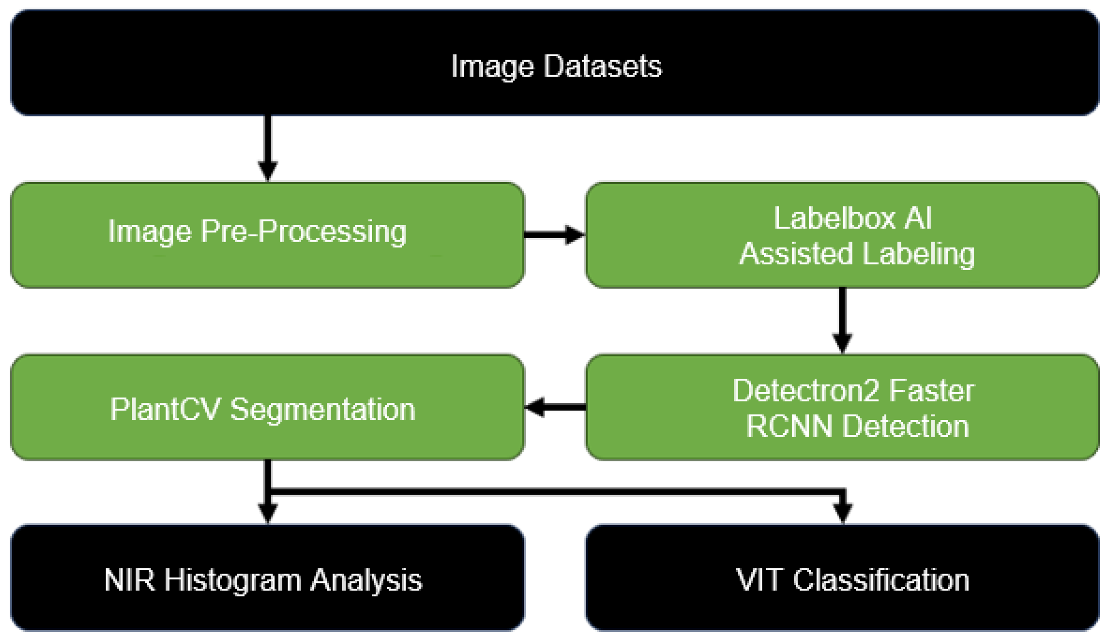
The overall processing pipeline is shown in Figure 2.

3.1. Image Pre-Processing

First, image normalization was performed for each session, using the equation n o r m = ( x m i n x ) / ( m a x x m i n x ) . x , m i n x , and m a x x stand for pixel value, minimum pixel value, and maximum pixel value, respectively. The next step in data pre-processing included creating patches to separate the four plants and sorting them into well-watered and drought-stressed categories. This was carried out using a semi-automatic script that took advantage of the repetitive motion of the camera, with the locations indexed by the image ID. The script assigned a patch with the same height as that of the image and allowed the user to decide where to cut the image vertically to crop out the plant. This patch size was allowed to automatically propagate across the images for two consecutive horizontal scans, after which the user was prompted to choose a new vertical cut. This process was repeated for each day in a trial. The creation of the patches resulted in four folders, each containing images of one plant. Folders 1 and 3 contained images of well-watered plants (Plants 1 and 3). Similarly, Folders 2 and 4 contained patches of drought-stressed plants (Plants 2 and 4). Out of these four plants, our analysis was conducted on Plants 2 and 3 since they were the most visible throughout each scan session. Plants 1 and 4, being located towards either end of the row, appeared inconsistently in between image frames due to the horizontal motion and edge distortions of the camera (see Figure 1). As a result, only a few patches from Plants 1 and 4 were extracted and, hence, were left out of the analysis. Additionally views that either had no plant part visible or just the top of some leaves visible were also removed. This was again performed semi-automatically utilizing the repetitive movement of the camera.
In an attempt to scale up the data collection and conduct drought-stress analysis on multiple trials, additional challenges were faced that were not addressed in [15]. As mentioned in Section 1, the YEL of maize plants has been shown to be significantly impacted by water stress. While we still wanted to rely on analysis of NIR pixels extracted from the YEL, accurately and consistently detecting the smallest leaf posed a significant challenge in our pre-processing steps. Being small and usually hidden between surrounding leaves, the YEL is usually difficult to detect in images. Also, occasional shifting of pots in the chamber at the time of watering and manual measurements as well as movement of the camera in each session led to images with changing views of the plants. Another major drawback present in the dataset was the significant overlap between leaves of adjacent plants, particularly in the later days of a trial when leaves were overgrown or at their maximum length. This led to occlusions of parts of the plant, which negatively impacted our analysis.
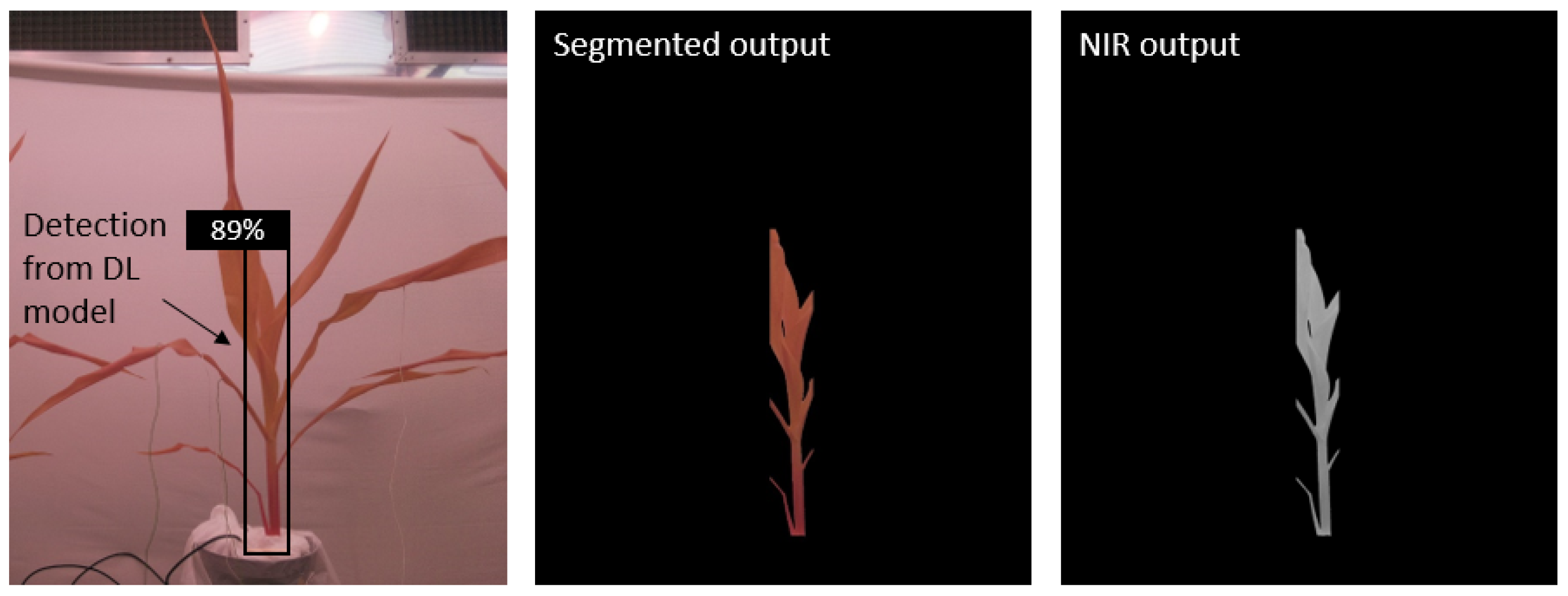
In order to overcome the above challenges, a different approach was adopted in our analysis than the one undertaken in [15]. Instead of training an object detection model to detect just the YEL, a region that approximately surrounded the YEL and the stem for each plant was chosen. Whenever the YEL was not visible, we annotated what we considered to be the next-youngest expanding leaf. Annotations were performed by drawing tight bounding boxes that enclosed the tip of the youngest leaf to the base of the stem. Figure 3 provides an example of the detections using our deep learning (DL) model. The online labeling platform LabelBox [25] was used for generating the ground-truth bounding boxes. Labelbox is a powerful labeling tool that allows efficient and accurate annotations of datasets for various machine learning projects. Through its online platform and easy-to-use interface, users can import data, define labels and annotation types, collaborate with team members to assign, annotate and review labels, and export the labeled data in the desired format. Additionally, LabelBox’s Model-Assisted Labeling (MAL) feature can significantly reduce annotation time by allowing computer-generated predictions to be uploaded as pre-labels. This feature proved especially useful in our analysis as it helped us to annotate our dataset in a short amount of time as well as to improve the detection accuracy.

3.2. Detection and Segmentation

Faster RCNN [26] is a popular object detection algorithm that has been used for a number of object detection tasks in the field of precision agriculture like weed [27] or multi-class fruit detection [28,29], identification of lettuce and sugarcane seedlings [30,31], and detection and segmentation of plant parts in maize [15,32]. Faster RCNN is comprised of two modules, including a Region Proposal Network (RPN), which is a fully convolutional network that generates proposals with various scales and aspect ratios. It applies the concept of attention in neural networks to guide the second module, which is a fast RCNN module, to look for objects in the image. Each region of proposals generated by the RPN is passed through an ROI pooling layer to extract a fixed-length feature vector. The extracted feature vectors are then classified using fast RCNN through classification scores and bounding box regression. Although no longer state of the art, the pipeline is still extremely effective and architecture agnostic and is, thus, a robust starting point for any object detection application. In our work, Facebook’s Detectron2 framework [26] was utilized, with a Faster RCNN backbone for the purpose of detection of the YEL and stem regions within each plant patch. For training our Detectron2 model, a curated dataset was used, combining our three imaging trials.
Two views from each vertical scan from the first sessions for each day were selected from all three trials. The two views were selected such that one showed the plant in full view while another showed the plant with the camera shifted up by a few vertical steps. Annotations were performed on the entire image instead of annotating the patches of individual plants. Table 2 shows details of our annotation process using Labelbox and its MAL feature. For each trial, a small subset of images was selected and labeled manually. The Detectron2 model was trained on this subset with a train–validation split of 90–10%, and the annotation time and model evaluation are reported in terms of average precision (AP and AP75 values). The predictions from this trained model were then used as pre-labels on a second set of images (using MAL), and the annotation time was compared with the manually labeled subset. It was observed that, with MAL, twice the number of images were annotated in less than half the time compared to manual labeling. The evaluation of our three final trained models with the full dataset (combining manually labeled and MAL images) are also reported. Due to a higher number of images in this case, a significant improvement is seen in the AP values. The three trained models were then used to run inference on all patches of individual plants in their respective trials. The predictions were used to extract the YEL and stem region from each plant. The extracted regions from Plant 2 (drought stressed) and Plant 3 (well-watered) were used in our subsequent analysis.
For segmenting the plant part within these regions, a method similar to the NIR workflow in PlantCV [20] was adopted. NIR images comprise grayscale pixels representing NIR light reflected from plants, requiring adequate lighting and sufficient contrast between plants and the background. To conduct water-stress analysis, the NIR channel from the NGB image was extracted, as depicted in Figure 3. Initially, the NGB image is converted to the Hue-Saturation-Value (HSV) scale using the OpenCV library [33]. Next, a binary mask is created using the saturation channel from the HSV image and the OpenCV thresholding techniques to eliminate the background. Finally, this binary mask is applied to the NIR image to obtain a masked NIR image with the background removed.

3.3. Drought-Stress Analysis

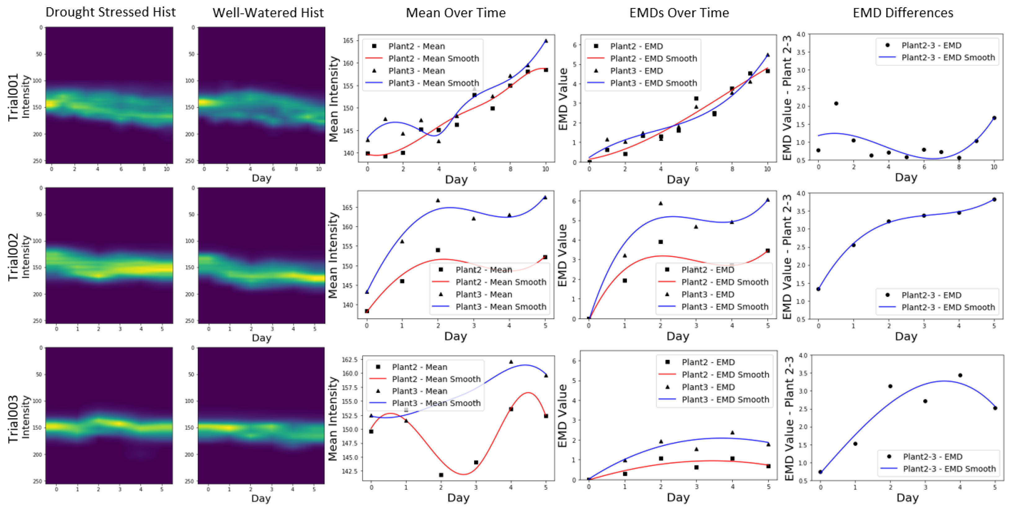
An analysis on the NIR values was performed over time by tracking changes in their distributions for the control and drought-stressed plants. The segmented NIR images were then used as inputs to a DL classifier, quantifying its performance over time as a way to monitor differences in the plants. For the first analysis, to study the distributions of the NIR pixels extracted from the detected regions, histograms and EMDs were computed. The shape of the histograms as well as their mean help us to visualize the pixel distributions of each plant as we progress through the days of the trial. Additionally, the EMDs capture how reflectance evolved for each plant over time by comparing each day with the first day of the trial.
The segmented plants were used to train a DL classifier to separate drought-stress and well-watered plants. A Vision Transformer (ViT) [22] was used to perform the binary classification. The transformer architecture is considered to be the state of the art for natural language processing and computer vision tasks. A ViT is a model based on the transformer architecture that performs image classification based on patches of images. It divides an image into fixed-size patches and adds positional embedding to these patches, which are then used as an input to the transformer encoder. ViTs have achieved the best results in various computer vision tasks like image classification, object detection and semantic segmentation. They are known to outperform CNNs from the literature like Big Transfer (BiT) [34], which performs supervised transfer learning with large resnets, and Noisy Student [35] which is a large EfficientNet trained using semi-supervised learning on ImageNet and JFT300M. Like the original transformer, ViTs are also equipped with the self-attention mechanism that allows one to capture long-range dependencies and contextual information present in the input data. The self-learned attention weights allow the model to focus on relevant areas in the image and provide more interpretability in the form of attention heatmaps. In Section 4 some attention plots are shown, indicating what our trained ViT has learned.
In order to quantify the impact of having the adjacent leaves as part of both analysis pipelines, the widths of the bounding boxes were increased. They were expanded on both sides by n = 200 , 400 , 700 , and 1000 pixels. This generates bounding boxes B 0 through B 4 . Figure 4 illustrates the original detected bounding box and the subsequent gradual expansion. The motivation behind conducting these experiments was to find a suitable bounding box size that encompassed the YEL and stem regions of the plants, which would yield the best results for drought-stress detection. It was also carried out to verify the negative effect of leaf occlusion by adjacent plants, as bounding boxes with larger widths were expected to perform worse.

4. Results

4.1. Implementation Details

To select training views for the ViT classifier, some views for each trial were separated based on the protocol adopted for the Detectron2 training, as discussed in Section 3.2. This gave us a total of 1278 images in the training set. A train–validation split of 85–15% was used. The remaining images were used as the test set. A total of six experiments were considered, using different combinations of trials for training and testing. Table 3 shows the details. Note that Trial 1 was not included as the train set for Experiments D and E, for reasons discussed later in the next subsection.
Transfer learning was used to fine-tune the ViT model pre-trained on ImageNet-21k at a resolution of 224 × 224 . Training was performed over 100 epochs with a batch size of 32. Data augmentation on the train set included horizontal flip, rotation, zoom, and brightness adjustment. An ADAM optimizer [36] with a learning rate of 5 × 10 5 was used for training. All experiments were run on an Ubuntu workstation with an NVIDIA GeForce GTX 1080 Ti GPU.

4.2. Results and Discussion

In this section, the results of our detailed analysis on our three imaging trials is presented. First, the results for our extracted NIR pixels are shown in the form of histogram distributions and EMD and then in the form of our ViT experiments with classification accuracy plots.
Figure 5 shows histograms and the mean of the distributions for the three trials, as well as the EMDs between the well-watered and drought-stressed groups. For the histogram plots, NIR intensity and time are plotted along the y and x axes, respectively, and the frequency is represented by the colors. The mean of the histograms over time are also plotted. The EMDs over time compare EMD each day with the first day of the experiment for both groups of plants. This gives an estimate of how the NIR reflectance evolves for each plant over time. The EMD differences show a cross-comparison between the well-watered and the drought-stressed plants per day. To smooth the data values, a spline representation and B spline basis elements are implemented, utilizing scipy’s interpolation package [37]. No separation between the groups for Trial 1 is observed. One of the possible explanations for this is that Trial 1 had almost twice the number of days compared to the other trials. This prolonged period of drought stress could be a reason why expected trends were not observed. A higher number of days also meant that plants were overgrown towards the end of the trial, which led to more occlusion and, in turn, more noisy data. Furthermore, evaporation and stomatal conductance are very dynamic and can change not only with plant dehydration, but also with light, temperature, vapor pressure deficit (VPD), etc. In a controlled chamber setting, even though it is possible to control most of these parameters, some, like VPD, are prone to significant fluctuations, which, in turn, can affect plant transpiration rate and photosynthesis [38,39,40].
Trial 2 showed the overall best separation between the two distributions. We observe a clear separation between the means of the NIR pixel distributions as well as the EMD over time plot. The EMD difference between the two sets of plants also shows a continuous increase as we progress through the trial. For Trial 3, even though a separation can be observed in all of the plots, this is not as clear as in the case of Trial 2. It can be observed that the separation between the plants decreases towards the end of the trial, as seen in the mean over time plot. Unlike Trial 2, the EMD values for each plant do not show a sharp increase compared to the first day of the trial.
The EMD cross-comparison between the two plants also shows a slight dip in the otherwise increasing curve, towards the end of the trial. These results could be attributed to more leaf occlusions present in Trial 3 in comparison to Trial 2.
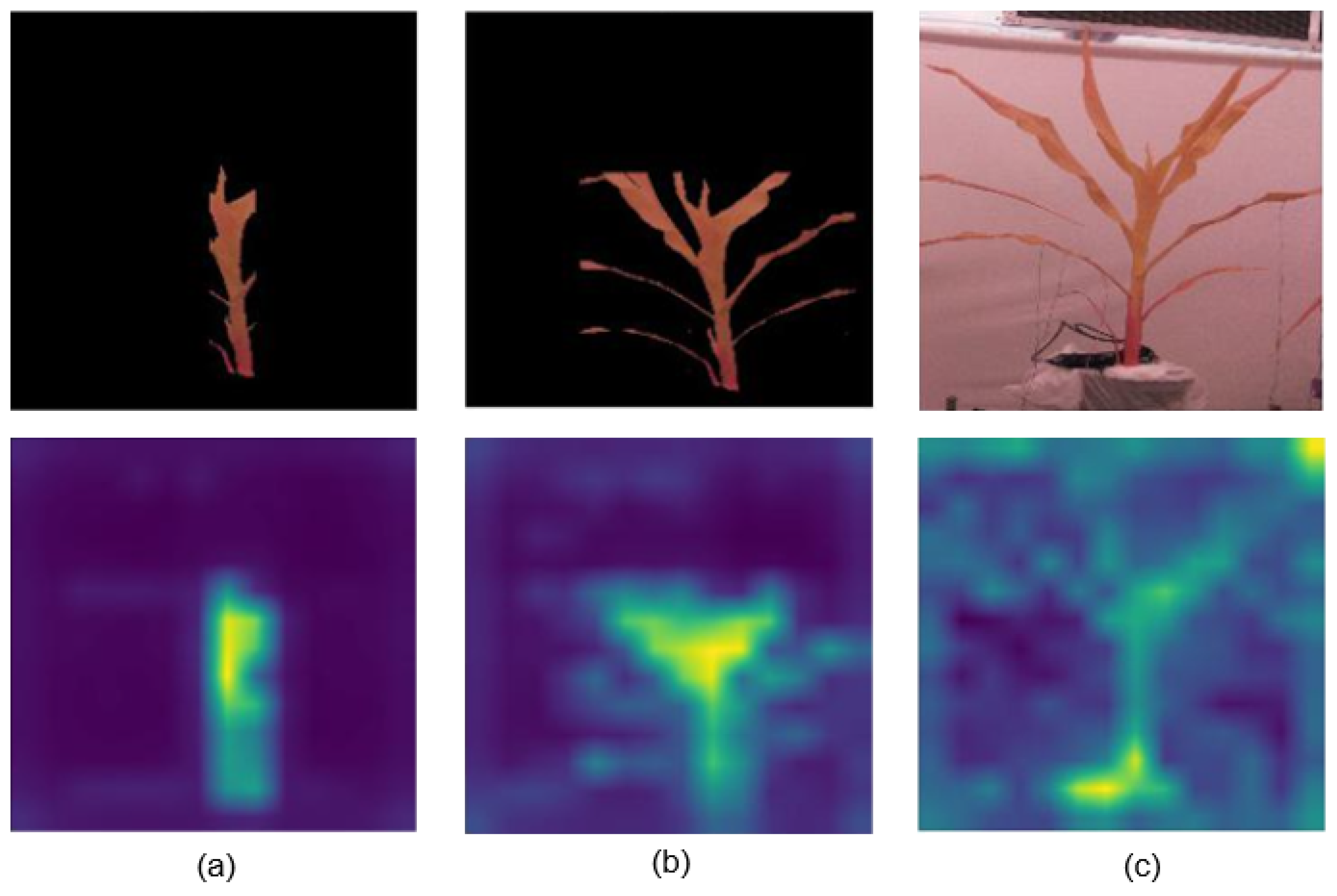
For the classification task, Figure 6 shows attention masks extracted from the self-attention layers of our ViT. Maximum brightness is seen around the YEL region for both sets of images, indicating that this region of the plants is most sensitive to changes in the watering regime. An example of what the ViT is learning from images that do not have the background segmented out is also shown. It is observed that the attention in this scenario is no longer near the YEL region but on other parts of the background. To prevent the model from learning to identify objects on the background, our ViT classifier was trained on images with the background removed.
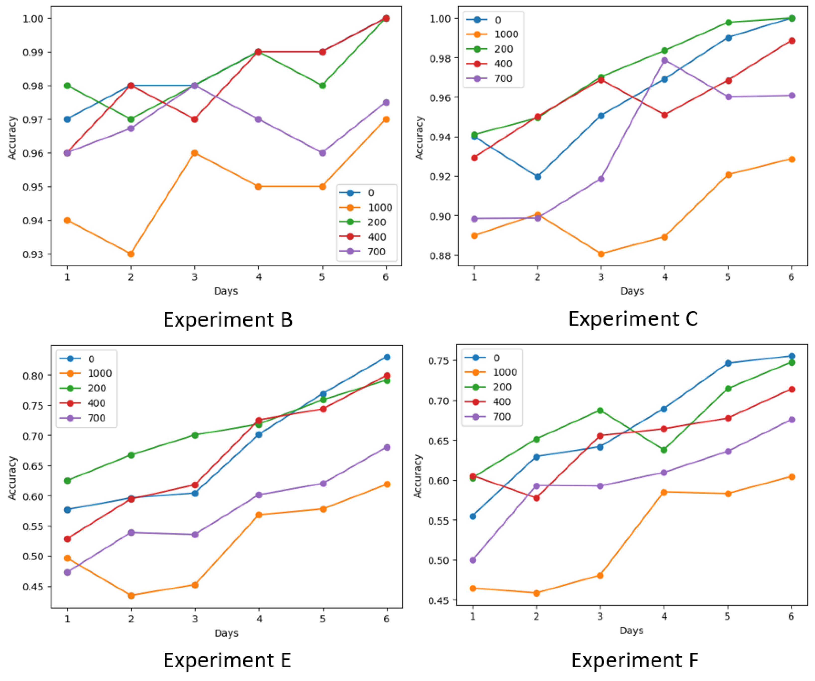
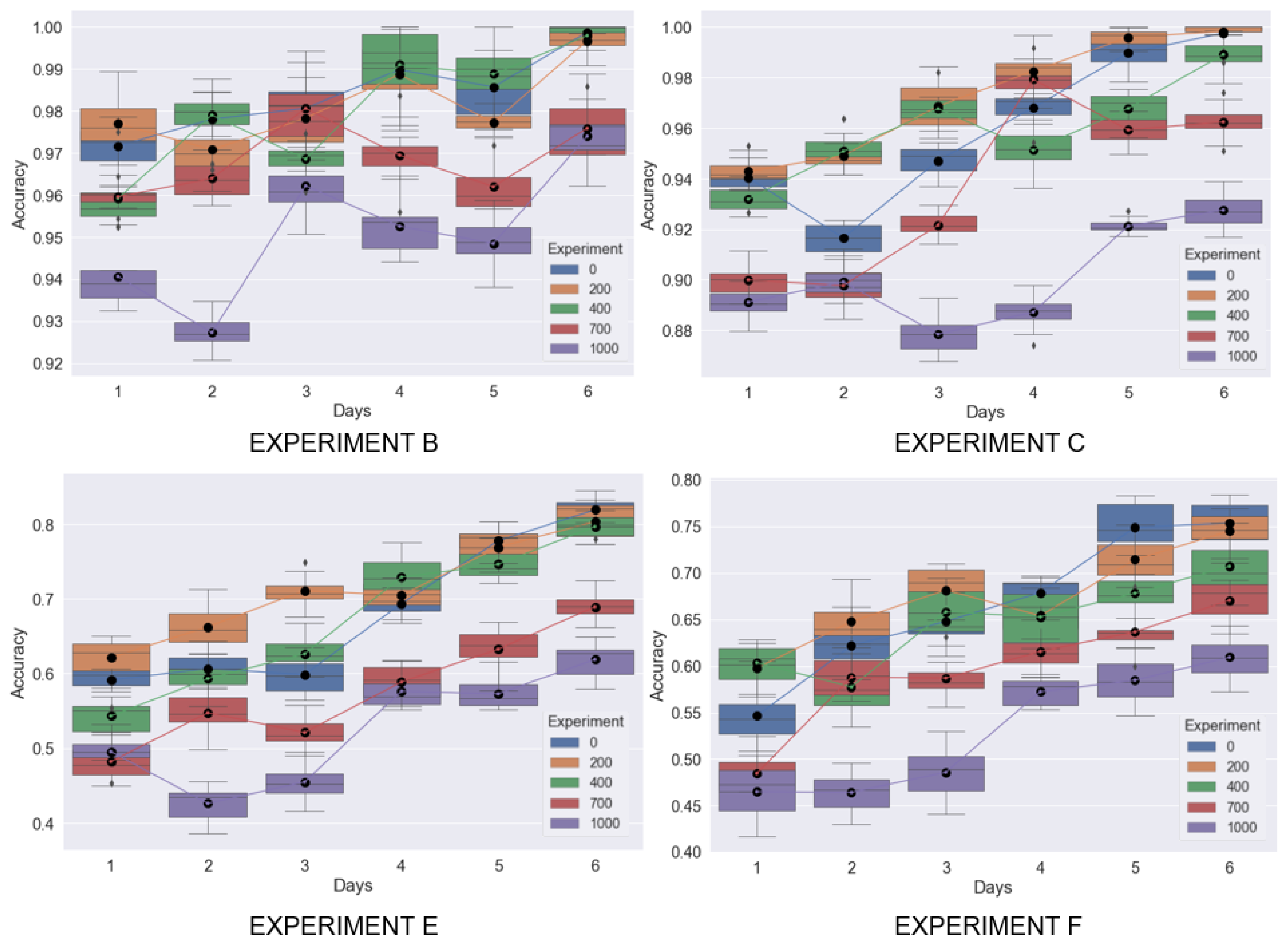
Figure 7 shows classification accuracy for the different combinations of train and test images introduced in Table 3. In order to obtain smoother trends, we performed multiple model runs of our ViT classifier corresponding to each bounding box. Each model was run 10 times, and boxplots of the classification accuracy over time were generated for each trial and are shown in Figure 8. Table 3 shows mean and standard deviation values for bounding box B 0 . Mean1 and STD1 are values averaged over all runs and all days of the test trial. Mean2 and STD2 show the values averaged over all runs for the last day of each test trial. For experiments A, B, and C, selected train views from all trials are combined and tested on each trial separately. As a result, an overall high classification accuracy is achieved for these experiments.
Similar to the NIR pixel analysis results, a much lower mean accuracy for Experiment D (tested on Trial 1) is observed. Overall, for Trial 1, a clear separation between the two sets of plants was not observed and, hence, boxplots for A and D are not shown. In Figure 7 B, C, all trials are combined for training, and testing is performed on Trials 2 and 3, respectively. E and F show results on Trials 2 and 3, respectively, when trained on a different trial. Compared to B and C, there is an overall drop in accuracy for these experiments, as hold-out trials are introduced for testing.
For E and F, a gradual increase in accuracy is observed as one moves from the first day to the last day of the trial. Such a trend is expected, as, over time, the drought stress becomes prolonged, thus creating a larger separation between the two groups. This presumably makes it easier for the model to classify the two sets of plants as the trial progresses. This increasing trend across the trial is also slightly observable in B and C.
A second trend observed in B, C, E, and F is a drop in accuracy for bounding boxes B 3 and B 4 when compared to B 0 , B 1 , and B 2 . Particularly, for bounding box B 4 , which includes the entire plant for classification, a significant drop in accuracy can be seen for most days in the trial. This is also expected, as a full view of the plant includes more occlusions from the leaves of adjacent plants, which are treated with the opposite watering protocol. These occlusions are absent or quite small for bounding boxes B 0 , B 1 , and B 2 , which is why overall accuracy is higher for these sets of images. Overall, Trial 2 performs better than Trial 3 for both experiments involving hold-out or no hold-out test trials. For Trial 2, the highest classification accuracy of 85% was observed on the last day of the trial for bounding box B 0 . In comparison, the highest classification accuracy for Trial 3 was observed to be 78.4%. From these experiments, it can be concluded that, in controlled chamber settings and through a multi-analysis approach, early drought-stress detection from NIR images of maize plants is possible before it becomes evident through visual inspection.

5. Conclusions

In this paper, an existing high-throughput low-cost system developed by [15] is used for water-stress detection from NIR images of maize plants. In our effort to scale up the analysis on more imaging trials, additional challenges were faced that are not addressed by the authors in [15]. These challenges involved difficulties in annotating and detecting the YEL of the plants as well as the occlusion of leaves by adjacent plants. To overcome these, a pipeline for automatic detection of drought stress is introduced. This approach did not solely rely on the YEL but instead focused on the region surrounding the YEL and the stem. Our analysis on three imaging trials revealed several key findings. Using extracted NIR pixel values, we computed histograms and EMD values for all three trials. Clear separations between the histograms and EMD values were observed for the two sets of plants for Trials 2 and 3. The Vision Transformer, implemented for classifying drought-stressed and well-watered plants, showed an increase in accuracy across the days of the trial, which could be correlated to an increase in drought stress from the first to last day of the trial. Our bounding box experiments also showed a significant drop in accuracy in the case of analysis on the entire plant vs. areas surrounding the YEL and the stem region. It was shown that this region can act as a more reliable alternative to the YEL. Our hold-out test trial experiments gave classification accuracy of 85% and 78.4% for Trials 2 and 3, respectively, corresponding to the last day of the trial and bonding box B 0 . Overall, out of the three trials performed, early drought-stress detection was clearly observable in two of them based on our classification metric and NIR distribution analysis. We intend to use our pipeline for remote monitoring of plants in controlled chamber settings, which could aid future research in the field of crop science.

Author Contributions

Conceptualization: M.D., A.B. and E.L.; Methodology: S.B. and E.L.; Software: S.B.; Experiments: J.R. and M.T.; Data curation: J.R., M.T. and S.B.; Writing—original draft preparation: S.B.; Writing—review and editing: J.R., M.T., M.D., A.B. and E.L.; Supervision: M.D., A.B. and E.L. All authors have read and agreed to the published version of the manuscript.

Funding

This work was supported by the United States Department of Agriculture—National Institute of Food and Agriculture under grant number 1015796 and the United States National Science Foundation under grant numbers ECCS-2231012, EF-2319389, ITE-2344423, IIS-2037328, and EEC-1160483 for the Nanosystems Engineering Research Center for Advanced Self-Powered Systems of Integrated Sensors and Technologies (ASSIST).

Data Availability Statement

The original data presented in the study are openly available on the data sharing platform Zenodo https://zenodo.org/records/10991581 (accessed on 18 April 2024) with DOI 10.5281/zenodo.10991581. The repository contains raw images before any of the pre-processing steps mentioned in Section 3. Images in the repository were down-sampled from their original resolution (see Section 2) by a factor of 2 due to a size restriction on Zenodo. The resized dataset is 16.8 GB. For any other questions about the dataset or data availability, please reach out to the corresponding author.

Acknowledgments

The authors would like to thank Carole Saravitz, Joe Chiera, and other staff members at the NC State University Phytotron for their assistance with plant care and chamber maintenance.

Conflicts of Interest

The authors declare no conflicts of interest. The funders had no role in the design of the study; in the collection, analyses, or interpretation of data; in the writing of the manuscript; or in the decision to publish the results.

References

  1. Sheoran, S.; Kaur, Y.; Kumar, S.; Shukla, S.; Rakshit, S.; Kumar, R. Recent advances for drought stress tolerance in maize (Zea mays L.): Present status and future prospects. Front. Plant Sci. 2022, 13, 872566. [Google Scholar] [CrossRef]
  2. Goyal, P.; Sharda, R.; Saini, M.; Siag, M. A deep learning approach for early detection of drought stress in maize using proximal scale digital images. Neural Comput. Appl. 2024, 36, 1899–1913. [Google Scholar] [CrossRef]
  3. Gao, Y.; Qiu, J.; Miao, Y.; Qiu, R.; Li, H.; Zhang, M. Prediction of leaf water content in maize seedlings based on hyperspectral information. IFAC-PapersOnLine 2019, 52, 263–269. [Google Scholar] [CrossRef]
  4. An, J.; Li, W.; Li, M.; Cui, S.; Yue, H. Identification and classification of maize drought stress using deep convolutional neural network. Symmetry 2019, 11, 256. [Google Scholar] [CrossRef]
  5. Zhuang, S.; Wang, P.; Jiang, B.; Li, M.; Gong, Z. Early detection of water stress in maize based on digital images. Comput. Electron. Agric. 2017, 140, 461–468. [Google Scholar] [CrossRef]
  6. Jiang, B.; Wang, P.; Zhuang, S.; Li, M.; Li, Z.; Gong, Z. Detection of maize drought based on texture and morphological features. Comput. Electron. Agric. 2018, 151, 50–60. [Google Scholar] [CrossRef]
  7. Asaari, M.; Mertens, S.; Dhondt, S.; Inzé, D.; Wuyts, N.; Scheunders, P. Analysis of hyperspectral images for detection of drought stress and recovery in maize plants in a high-throughput phenotyping platform. Comput. Electron. Agric. 2019, 162, 749–758. [Google Scholar] [CrossRef]
  8. Souza, A.; Yang, Y. High-throughput corn image segmentation and trait extraction using chlorophyll fluorescence images. Plant Phenomics 2021, 2021, 9792582. [Google Scholar] [CrossRef]
  9. Romano, G.; Zia, S.; Spreer, W.; Sanchez, C.; Cairns, J.; Araus, J.; Müller, J. Use of thermography for high throughput phenotyping of tropical maize adaptation in water stress. Comput. Electron. Agric. 2011, 79, 67–74. [Google Scholar] [CrossRef]
  10. Gausman, H.; Allen, W. Optical parameters of leaves of 30 plant species. Plant Physiol. 1973, 52, 57–62. [Google Scholar] [CrossRef]
  11. Humplík, J.; Lazár, D.; Husičková, A.; Spíchal, L. Automated phenotyping of plant shoots using imaging methods for analysis of plant stress responses—A review. Plant Methods 2015, 11, 29. [Google Scholar] [CrossRef] [PubMed]
  12. Hsiao, T.; Acevedo, E.; Henderson, D. Maize leaf elongation: Continuous measurements and close dependence on plant water status. Science 1970, 168, 590–591. [Google Scholar] [CrossRef]
  13. Acevedo, E.; Hsiao, T.; Henderson, D. Immediate and subsequent growth responses of maize leaves to changes in water status. Plant Physiol. 1971, 48, 631–636. [Google Scholar] [CrossRef] [PubMed]
  14. Tardieu, F.; Reymond, M.; Hamard, P.; Granier, C.; Muller, B. Spatial distributions of expansion rate, cell division rate and cell size in maize leaves: A synthesis of the effects of soil water status, evaporative demand and temperature. J. Exp. Bot. 2000, 51, 1505–1514. [Google Scholar] [CrossRef] [PubMed]
  15. Silva, R.; Starliper, N.; Bhosale, D.; Taggart, M.; Ranganath, R.; Sarje, T.; Daniele, M.; Bozkurt, A.; Rufty, T.; Lobaton, E. Feasibility study of water stress detection in plants using a high-throughput low-cost system. In Proceedings of the 2020 IEEE SENSORS, Rotterdam, The Netherlands, 25–28 October 2020; pp. 1–4. [Google Scholar]
  16. Valle, B.; Simonneau, T.; Boulord, R.; Sourd, F.; Frisson, T.; Ryckewaert, M.; Hamard, P.; Brichet, N.; Dauzat, M.; Christophe, A. PYM: A new, affordable, image-based method using a Raspberry Pi to phenotype plant leaf area in a wide diversity of environments. Plant Methods 2017, 13, 98. [Google Scholar] [CrossRef] [PubMed]
  17. Lee, U.; Chang, S.; Putra, G.; Kim, H.; Kim, D. An automated, high-throughput plant phenotyping system using machine learning-based plant segmentation and image analysis. PLoS ONE 2018, 13, e0196615. [Google Scholar] [CrossRef] [PubMed]
  18. Brichet, N.; Fournier, C.; Turc, O.; Strauss, O.; Artzet, S.; Pradal, C.; Welcker, C.; Tardieu, F.; Cabrera-Bosquet, L. A robot-assisted imaging pipeline for tracking the growths of maize ear and silks in a high-throughput phenotyping platform. Plant Methods 2017, 13, 1–12. [Google Scholar] [CrossRef] [PubMed]
  19. Ren, S.; He, K.; Girshick, R.; Sun, J. Faster r-cnn: Towards real-time object detection with region proposal networks. Adv. Neural Inf. Process. Syst. 2015, 28, 1–9. [Google Scholar] [CrossRef] [PubMed]
  20. Gehan, M.; Fahlgren, N.; Abbasi, A.; Berry, J.; Callen, S.; Chavez, L.; Doust, A.; Feldman, M.; Gilbert, K.; Hodge, J.; et al. PlantCV v2: Image analysis software for high-throughput plant phenotyping. PeerJ 2017, 5, e4088. [Google Scholar] [CrossRef]
  21. Rubner, Y.; Tomasi, C.; Guibas, L. A metric for distributions with applications to image databases. In Proceedings of the Sixth International Conference on Computer Vision (IEEE Cat. No. 98CH36271), Bombay, India, 7 January 1998; pp. 59–66. [Google Scholar]
  22. Dosovitskiy, A.; Beyer, L.; Kolesnikov, A.; Weissenborn, D.; Zhai, X.; Unterthiner, T.; Dehghani, M.; Minderer, M.; Heigold, G.; Gelly, S.; et al. An image is worth 16 × 16 words: Transformers for image recognition at scale. arXiv 2020, arXiv:2010.11929. [Google Scholar]
  23. Raspberry pi Hardware Documnetation. Available online: https://www.raspberrypi.com/documentation/computers/raspberry-pi.html (accessed on 30 May 2024).
  24. Node-RED [Online]. Available online: https://nodered.org/ (accessed on 30 May 2024).
  25. Labelbox, “Labelbox”, Online, 2024. Available online: https://labelbox.com (accessed on 30 May 2024).
  26. Wu, Y.; Kirillov, A.; Massa, F.; Lo, W.Y.; Girshick, R. Detectron2. 2019. Available online: https://github.com/facebookresearch/detectron2 (accessed on 30 May 2024).
  27. Le, V.; Truong, G.; Alameh, K. Detecting weeds from crops under complex field environments based on Faster RCNN. In Proceedings of the 2020 IEEE Eighth International Conference on Communications and Electronics (ICCE), Phu Quoc, Vietnam, 13–15 January 2021; pp. 350–355. [Google Scholar]
  28. Gao, F.; Fu, L.; Zhang, X.; Majeed, Y.; Li, R.; Karkee, M.; Zhang, Q. Multi-class fruit-on-plant detection for apple in SNAP system using Faster R-CNN. Comput. Electron. Agric. 2020, 176, 105634. [Google Scholar] [CrossRef]
  29. Wan, S.; Goudos, S. Faster R-CNN for multi-class fruit detection using a robotic vision system. Comput. Netw. 2020, 168, 107036. [Google Scholar] [CrossRef]
  30. Li, Z.; Li, Y.; Yang, Y.; Guo, R.; Yang, J.; Yue, J.; Wang, Y. A high-precision detection method of hydroponic lettuce seedlings status based on improved Faster RCNN. Comput. Electron. Agric. 2021, 182, 106054. [Google Scholar] [CrossRef]
  31. Pan, Y.; Zhu, N.; Ding, L.; Li, X.; Goh, H.; Han, C.; Zhang, M. Identification and counting of sugarcane seedlings in the field using improved faster R-CNN. Remote. Sens. 2022, 14, 5846. [Google Scholar] [CrossRef]
  32. Liu, Y.; Cen, C.; Che, Y.; Ke, R.; Ma, Y.; Ma, Y. Detection of maize tassels from UAV RGB imagery with faster R-CNN. Remote Sens. 2020, 12, 338. [Google Scholar] [CrossRef]
  33. Bradski, G. The OpenCV Library. In Dr. Dobb’s Journal of Software Tools; Miller Freeman Inc.: San Francisco, CA, USA, 2000. [Google Scholar]
  34. Kolesnikov, A.; Beyer, L.; Zhai, X.; Puigcerver, J.; Yung, J.; Gelly, S.; Houlsby, N. Big transfer (bit): General visual representation learning. In Proceedings of the Computer Vision–ECCV 2020: 16th European Conference, Glasgow, UK, 23–28 August 2020; Proceedings, Part V 16. 2020; pp. 491–507. [Google Scholar]
  35. Xie, Q.; Luong, M.; Hovy, E.; Le, Q. Self-training with noisy student improves imagenet classification. In Proceedings of the IEEE/CVF Conference on Computer Vision and Pattern Recognition, Seattle, WA, USA, 13–19 June 2020; pp. 10687–10698. [Google Scholar]
  36. Kingma, D.; Ba, J. Adam: A method for stochastic optimization. arXiv 2014, arXiv:1412.6980. [Google Scholar]
  37. Virtanen, P.; Gommers, R.; Oliphant, T.; Haberland, M.; Reddy, T.; Cournapeau, D.; Burovski, E.; Peterson, P.; Weckesser, W.; Bright, J.; et al. SciPy 1.0 Contributors SciPy 1.0: Fundamental Algorithms for Scientific Computing in Python. Nat. Methods 2020, 17, 261–272. [Google Scholar] [CrossRef] [PubMed]
  38. Hsiao, J.; Swann, A.; Kim, S. Maize yield under a changing climate: The hidden role of vapor pressure deficit. Agric. For. Meteorol. 2019, 279, 107692. [Google Scholar] [CrossRef]
  39. Devi, M.; Reddy, V.; Timlin, D. Drought-induced responses in maize under different vapor pressure deficit conditions. Plants 2022, 11, 2771. [Google Scholar] [CrossRef]
  40. Inoue, T.; Sunaga, M.; Ito, M.; Yuchen, Q.; Matsushima, Y.; Sakoda, K.; Yamori, W. Minimizing VPD fluctuations maintains higher stomatal conductance and photosynthesis, resulting in improvement of plant growth in lettuce. Front. Plant Sci. 2021, 12, 646144. [Google Scholar] [CrossRef]
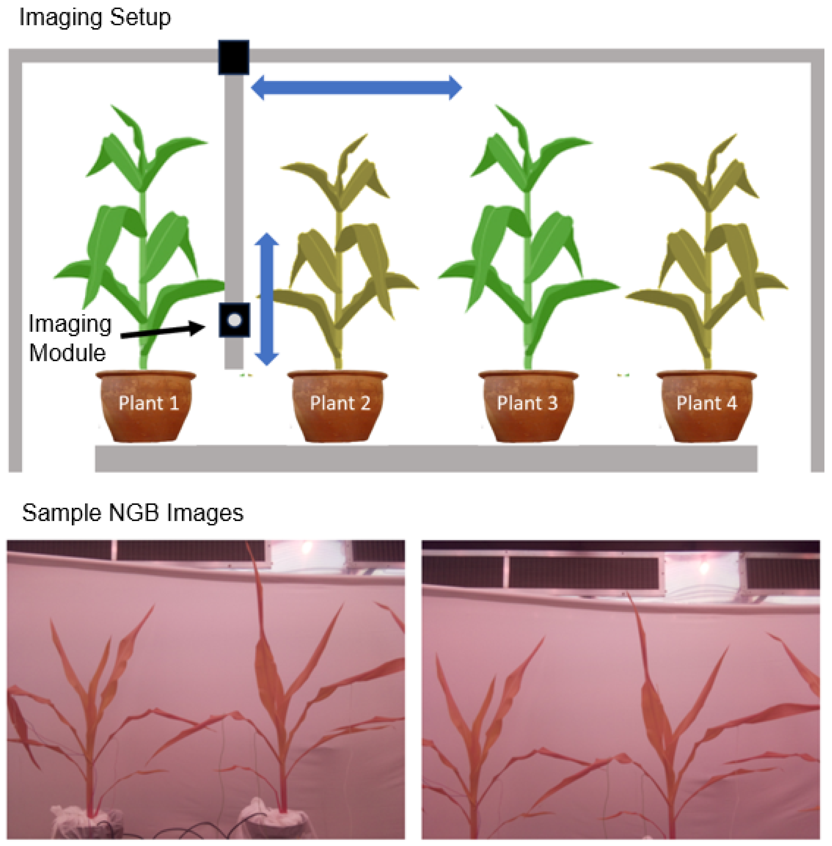
Figure 1. Plant Data Collection (PDC) system. [Top] Diagram of the imaging setup. A frame was built to house the imaging module that could translate horizontally and vertically to image the plant. Images were taken while sweeping the module vertically and horizontally. [Bottom] Sample NGB images taken from Trial 2 using the NoIR Pi Camera.
Ai 05 00040 g001
Figure 2. Pipeline adopted in our work for remote monitoring of plants inside a controlled chamber and early detection of induced drought stress.
Ai 05 00040 g002
Figure 3. NIR segmentation pipeline. [Left] Bounding box prediction using FasterRCNN. [Middle] Segmented portion of plant extracted from bounding box prediction. [Right] NIR channel extracted from NGB image.
Ai 05 00040 g003
Figure 4. Expanding bounding boxes. [Left] Overlay of the expanded bounding boxes containing the YEL and the stem. B 0 represents the original detection from the DL model, and B 1 B 4 are versions expanded on the left and right by 200, 400, 700, and 1000 pixels. [Right] Resulting segmentation for the corresponding expanded bounding boxes.
Ai 05 00040 g004
Figure 5. Histogram and EMD differences for B 0 bounding box. [Columns 1 and 2] NIR histograms are shown for the drought-stressed and well-watered plants on each trial. [Column 3] The means of the distribution are shown over time. The smooth mean values are obtained by applying a smoothing spline fitting to the data. [Column 4] The EMDs obtained by comparing the distributions over time to the initial distribution for each plant separately. [Column 5] The EMD obtained by comparing the distributions of the plants each day. We observed a similar trend for other bounding boxes.
Ai 05 00040 g005
Figure 6. Attention plots generated by our ViT binary classifier. Top row corresponds to original image, with the bottom row showing the corresponding attention maps. (a,b) correspond to bounding boxes B 0 and B 2 , respectively. (c) shows attention plots generated with the full plant in view and when the background is not segmented out. Objects around the plant are used as features for classification if not removed.
Ai 05 00040 g006
Figure 7. ViT classification accuracy for bounding boxes B 0 through B 4 for Experiments B, C, E, and F, as specified in Table 3.
Ai 05 00040 g007
Figure 8. Boxplots of classification accuracy for multiple model runs corresponding to bounding boxes B 0 through B 4 for Experiments B, C, E, and F, as specified in Table 3. For each experiment, we also show the means of the boxplots connected together.
Ai 05 00040 g008
Table 1. Details of our imaging trials.
TrialGrowth StageNo. of DaysV StepsH StepsNo. of ImagesDrydown Start
1V411402713,987Day 1
2V49402815,730Day 4
3V39292913,422Day 4
Table 2. Train image annotation using LabelBox and detection performance using Detectron2 library.
Trial 1Trial 2Trial 3
No MALMALNo MALMALNo MALMAL
No. of images200394100236100248
Annotation Time2 h 5 min48 min1 h 12 min29 min58 min32 min
No MALTotalNo MALTotalNo MALTotal
Detectron2 Perf (AP)75.3379.4178.1084.9277.9382.20
Detectron2 Perf (AP 75)90.579493.7196.3793.0496.05
Table 3. Train and test sets for the ViT model, along with mean and standard deviation values of classification accuracy for window B 0 . Averaging is performed across multiple model runs. Mean1 is averaged over all days in a trial, whereas Mean2 values correspond to the last day of the test trial.
ExperimentNo. of Train ImagesNo. of Test ImagesMean1STD1Mean2STD2
A1, 2, 3 (1278)1 (8635)0.97790.00610.98660.0082
B1, 2, 3 (1278)2 (5160)0.98410.00540.99870.0021
C1, 2, 3 (1278)3 (4818)0.95990.00620.99750.005
D2, 3 (684)1 (8635)0.56330.02310.66780.028
E3 (348)2 (5160)0.68150.01970.82110.022
F2 (336)3 (4818)0.66630.02430.75370.0255
Disclaimer/Publisher’s Note: The statements, opinions and data contained in all publications are solely those of the individual author(s) and contributor(s) and not of MDPI and/or the editor(s). MDPI and/or the editor(s) disclaim responsibility for any injury to people or property resulting from any ideas, methods, instructions or products referred to in the content.