Application of Machine Learning for Insect Monitoring in Grain Facilities

Abstract

In this study, a basic insect detection system consisting of a manual-focus camera, a Jetson Nano—a low-cost, low-power single-board computer, and a trained deep learning model was developed. The model was validated through a live visual feed. Detecting, classifying, and monitoring insect pests in a grain storage or food facility in real time is vital to making insect control decisions. The camera captures the image of the insect and passes it to a Jetson Nano for processing. The Jetson Nano runs a trained deep-learning model to detect the presence and species of insects. With three different lighting situations: white LED light, yellow LED light, and no lighting condition, the detection results are displayed on a monitor. Validating using F1 scores and comparing the accuracy based on light sources, the system was tested with a variety of stored grain insect pests and was able to detect and classify adult cigarette beetles and warehouse beetles with acceptable accuracy. The results demonstrate that the system is an effective and affordable automated solution to insect detection. Such an automated insect detection system can help reduce pest control costs and save producers time and energy while safeguarding the quality of stored products.

1. Introduction

While breeders and farmers strive for high-yielding grain varieties and increased crop production to meet the demand of the growing world population, up to 80% of total production is lost during harvesting, storage, and processing [1]. During storage, grain losses are estimated at 10–40% due to insect damage [2]. Insect infestation causes physical degradation (weight loss), grain quality and safety issues, and physical damage to storage structures and facilities, which all lead to health risks and economic loss [1,2,3].

Integrated Pest Management (IPM) has become the basis for insect management and control decisions in facilities where food and grain are processed or stored. IPM is based on insect ecology, and its operational plan has at least two key elements: monitoring-based decision-making and multiple pest control tactic applications. Given the challenges in finding and sampling insect populations directly in the temporal and spatial landscapes found in and around food facilities, monitoring relies on visual observation, or capture in traps, of dispersing adults. For stored insect pest prevention and control, various techniques and technologies have been explored and applied to identify, detect, and monitor insects in storage facilities. Commonly used are manual sampling traps and probes, manual inspection and sieving, the floatation method, kernel staining, uric acid measurement, the Berlese funnel method, acoustic techniques, X-ray imaging, and the solid-phase micro-extraction method, among others [4]. Most of these methods are destructive, subjective, slow, labor-intensive, and time-consuming; usually have low accuracy and efficiency; could be limited to a few insect pests or specific insect growth stages; and may not be applicable to real-time applications [4]. Insect pests are small and, superficially, look very similar, so it takes highly trained people to accurately identify the species and age captured in traps and determine their risk level. Finally, most traps are selective in their captures since different pheromones and kairomones attract species, sexes, and developmental stages, making it difficult to measure populations accurately.

There is continued interest in the development of automated insect monitoring systems for both food production and the storage of raw and processed foods, but currently available technologies have limited ability to identify critical pests or require a person to do the actual insect identification. The use of artificial intelligence (AI) for the identification and counting of insects is a promising method to address the need for speed, timeliness, and reliability of insect information required for improving IPM methods. Cameras and other non-invasive sensors can continuously perform observations, and advances in computer vision technology, coupled with deep learning algorithms, provide methods to make AI insect identification possible. Images used to train deep-learning models could provide estimates of insect abundance, biomass, and diversity. Among the recent techniques for non-destructive, real-time, and rapid insect detection, near-infrared (NIR) spectroscopy and machine vision are promising. NIR spectroscopy is reliable and accurate but cannot detect low levels of insect infestation and differentiate between live and dead insects [3]. The machine vision system has been used for insect detection and monitoring, providing more benefits than the other methods. Aside from stored insect pest recognition and detection, it has also been applied in plant disease detection and crop quality grading [5]. Images and other outputs from these sensors used to train deep learning models could provide estimates of insect abundance, biomass, and diversity.

Previous work has focused on orchards and outdoor environmental pests, mostly flying, with some work conducted on crawling insects found in warehouses. Shuman et al. [6], Flinn et al. [7], and Banga et al. [4] looked at stored grain insects, while Potamitis et al. [8], Wen et al. [9], and Zhong et al. [10] focused on outdoor flying insects, and Eliopoulos et al. [11] examined crawling insects. Behavioral studies of insects could have benefited from automated insect enumeration and identification [12,13,14]. Shen et al. [15] recommended that mathematical modeling of insect movement continues to be a critical area of entomology research in which automated monitoring could play a significant role.

Machine vision has constantly been evolving as a technique for insect detection in stored grains. One of the first studies published was on detecting insects and body parts in bulk wheat samples, which used pattern recognition and multivariate analysis and obtained more than 90% accuracy [16]. Different algorithms and improved systems were developed to achieve high throughput [17], reduce instrument and computational costs, allow easy data access and real-time monitoring, and cover different insect pest species [18]. Some benefits of utilizing machine vision include: (a) the ability to analyze images and videos much faster and with higher accuracy than humans, which makes it suitable for high-speed quality control, inspection, and sorting tasks; (b) the capability to perform tasks consistently without errors or fatigue, ensuring consistent results; (c) the ability to analyze images and videos without physical contact, making it suitable for inspecting hazardous or fragile materials; (d) the flexibility of programming machine vision systems to analyze a wide variety of images and videos, enabling them to be used for various applications; and (e) the potential to reduce labor costs and enhance productivity, making it a cost-effective option for many applications.

However, the use of machine vision also has some drawbacks, which consist of: (a) the complexity of designing and implementing the systems, which require expertise in both hardware and software; (b) the cost of developing and implementing the systems, especially for specialized applications; (c) the systems’ sensitivity to lighting conditions, which can affect the accuracy and consistency of their results; (d) the limited understanding of context and inability to make judgments based on experience or intuition of systems using machine vision; and (e) the limited applicability of the systems, especially for applications that require complex decision-making skills beyond image analysis.

More recently, machine vision was combined with machine learning for enhanced stored insect grain detection and classification accuracy [5]. One of the most widely used machine learning techniques is the convolutional neural network (CNN), which consists of a complex network structure and has the ability to execute convolution operations [19]. Shen et al. [15] applied a deep neural network to detect and identify six species of stored grain insects that were blended with grain and dockage materials. Although they achieved a high mean average precision (mAP) of 88%, they used different models for different insects and encountered issues such as one species being classified as two. Another insect detection system built on deep CNN focused on different insect sizes and obtained mAP up to 95%, but still, they only detected one insect species at a time [20].

Being able to detect, classify, and monitor insect pests present in a grain storage or food facility in real-time will be vital to decision-making and insect control. In our study, we aimed to develop a camera-based monitoring system to detect and identify crawling stored grain insect pests using CNN and validate the model using a live feed.

2. Materials and Methods

The list of hardware components for this project and the software solution to detect and identify insects in real time are described in the following sections, along with the testing. This basic system was tested on adult warehouse beetles (Trogoderma variabile) and cigarette beetles (Lasioderma serricorne (F.)) from a culture maintained at the USDA-ARS Center for Grain and Animal Health Research in Manhattan, KS, USA. These insect species were selected as the test cases because they are major insect pests in food processing facilities (equipment and structures) and food product warehouses, and they are morphologically different [21]. The adult cigarette beetle is 2 to 4 mm long, 1.25 to 1.5 mm wide, and light to dark brown. Their antennae are saw-like and have the same thickness from the base to the tip. The head is withdrawn under the insect when it is at rest or dead, giving the insect a characteristic humped appearance. Adult warehouse beetles are smaller than cigarette beetles, at about 2.7 to 3.5 mm in length, oval, and predominantly black, with dense, dark-brown scales or setae covering the hardened forewings or elytra.

2.1. Hardware Components

Raspberry Pi (RPi) version 4 (the mention of trade names or commercial products in this publication is solely for the purpose of providing specific information and does not imply recommendation or endorsement by the U.S. Department of Agriculture. USDA is an equal opportunity provider and employer) (Raspberry Pi Trading Ltd., Cambridge, UK) was used in the original design of this study. Following extensive testing, modifications, and the lack of computing resources, it was replaced with an NVIDIA Jetson Nano 4 GB developer kit (NVIDIA, Santa Clara, CA, USA) [22], which served as the primary Central Processing Unit (CPU). The Jetson Nano has a built-in, dedicated Graphical Processing Unit (GPU), and an external camera was mounted on the Camera Serial Interface (CSI) port. 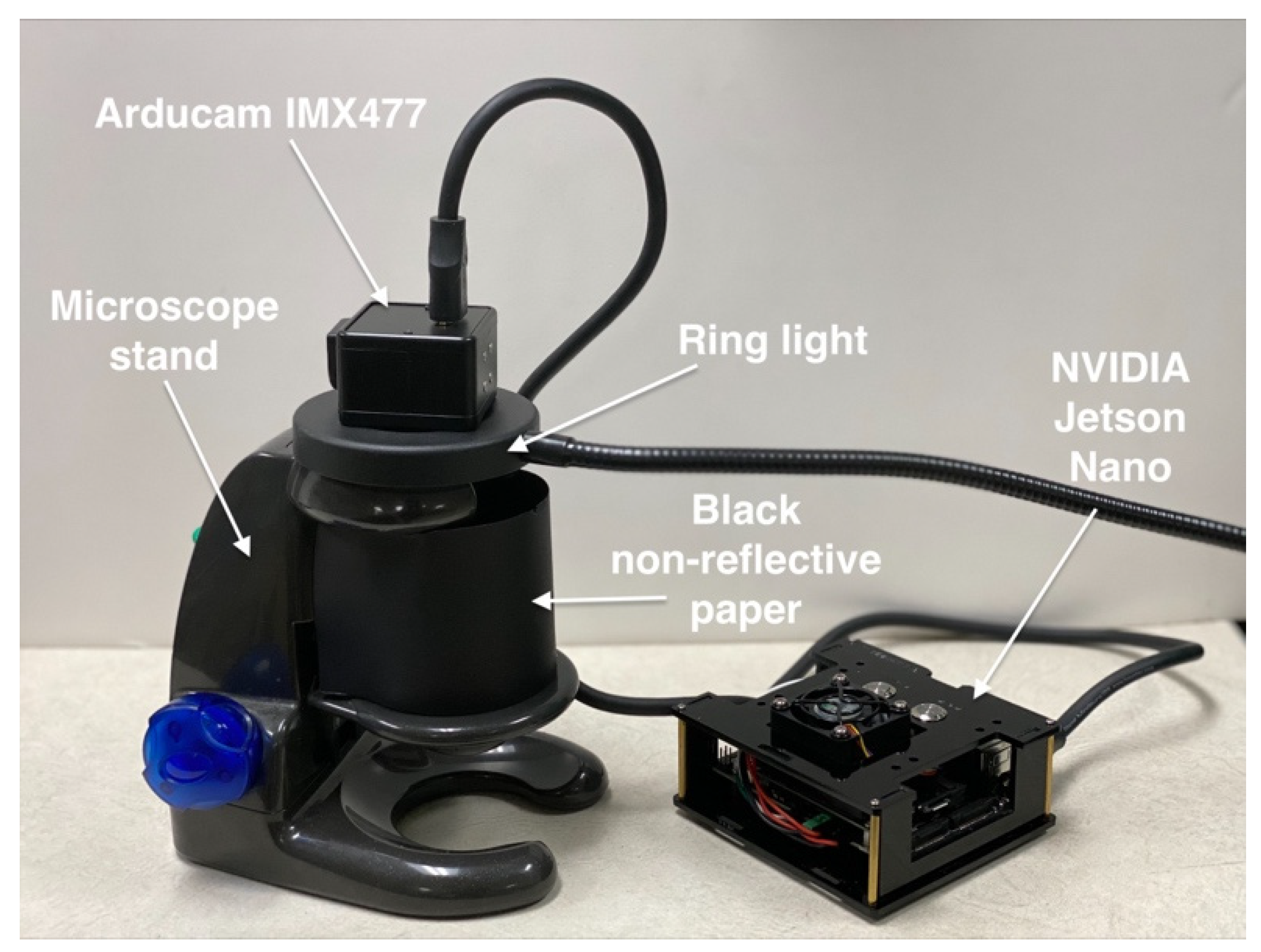The Arducam IMX477 B0250 model (ArduCAM, Nanjing, China) [23] was used for capturing images that also served as a medium for detection and identification. To reduce the chance of overheating while the GPU and CPU were simultaneously processing, a constant, on-demand cooling system was mounted on the Jetson Nano. A Universal Serial Bus (USB) ring light was also used for illumination, and black, non-reflective paper was used to cover the part where the insects were placed. As for the base, a microscope stand was used to adjust the height settings to calibrate the focus. Figure 1 shows how the hardware products were connected.

A regular keyboard, mouse, and external monitor were also connected to the Jetson Nano for initial configuration.

2.2. Software Solution

As part of the software package for the Jetson Nano, the NVIDIA JetPack (SD card image) 4.2 was used, and the procedures listed on the website of NVIDIA were followed. After the first boot for the initialization phase, software drivers for the Arducam were downloaded from their website for primary configuration. The compatibility of the CSI camera with the Jetson Nano must require no connectivity problems since it serves as our eyes in the field.

2.3. Preparing the Model

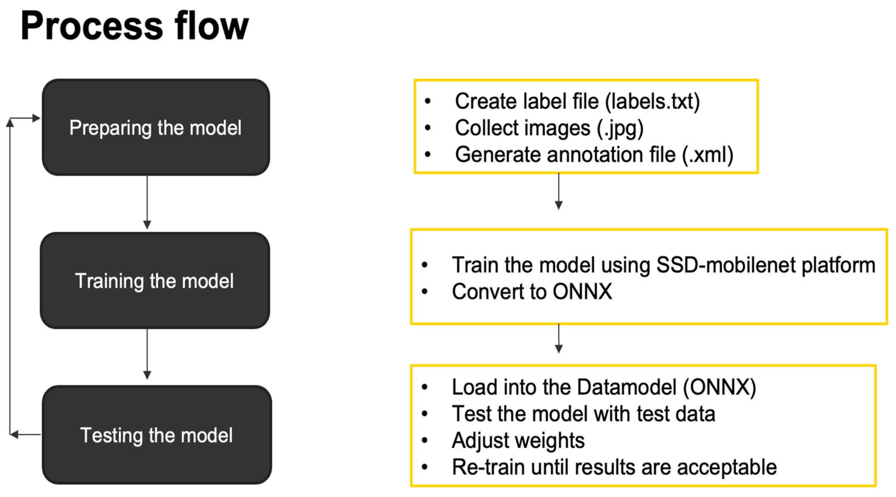
The gathering of data was the most tedious part of this project. The summary of the steps is presented in Figure 2. First, a label file was created, which was a text file containing the list of names of our insects (cigarette and warehouse beetles).

The next step was to capture images in JPG format. Two processes were used: first, images were downloaded from the internet (Figure 3) using basic data search, and second, using the CSI camera that was mounted on the Jetson Nano (Figure 4). Data augmentation was applied to each image. Data augmentation is a method of artificially expanding a dataset by applying various alterations to the existing samples. Data augmentation helps reduce overfitting in machine learning models and improves their ability to generalize to new data. In computer vision, popular data augmentation techniques include random cropping, flipping, rotations, translations, scaling, and color jittering. Training a model on a larger, augmented dataset can help it learn more robust features and generalize better to unseen data. It is frequently utilized when a model is trained to recognize objects or image patterns. The model may be taught to identify objects in various orientations, locations, and scales by applying random changes to existing photos. As a result, the model may be trained on a wider and more varied set of instances, which is particularly crucial for situations where there is little annotated data available.

More training data were produced by this process, which resulted in 1000 images (500 images for each insect classification), which were then segregated into 80–20 partitions: 80% for training data and 20% for test data (

Table 1. Partition of images per insect.

Insect Name	Scientific Name	Training Images	Test Images	Total
Cigarette beetle	Lasioderma serricorne	400	100	500
Warehouse beetle	Trogoderma variabile	400	100	500

). However, it is important to apply augmentation techniques relevant to the problem domain and to use them judiciously to avoid over-augmentation because this can lead to a loss of information and decrease model performance.

Generating an annotation file was the next step in preparing the model. It is important in machine learning because it provides labeled data to train the model. The model uses this data to learn the relationships between inputs and outputs and to make predictions. The annotations provide information about features and classes of the data, which are critical for creating accurate and effective models. Without annotated data, the model would have no way of learning the desired relationships and predictions and would likely perform poorly. 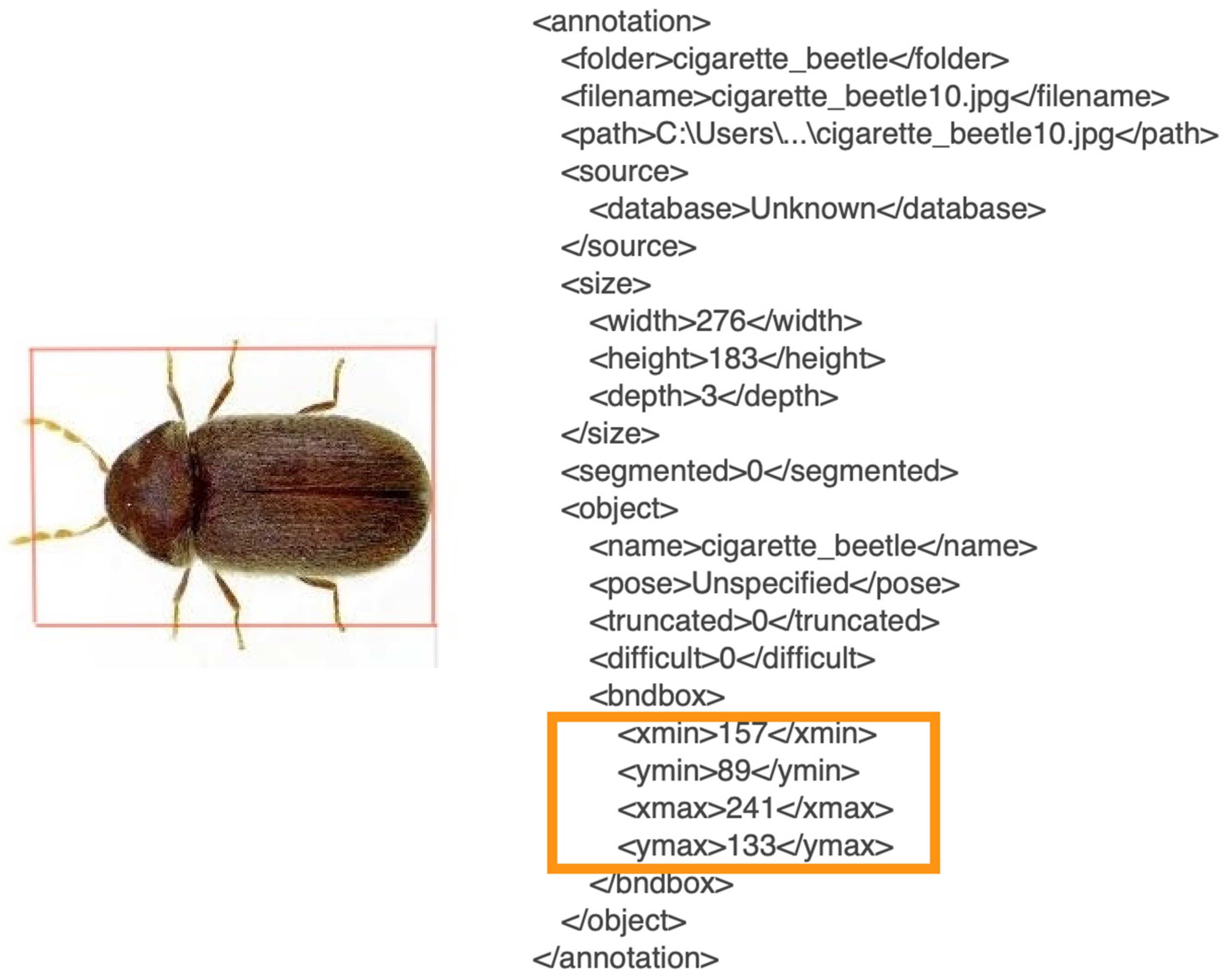In this part, the LabelImg (https://github.com/tzutalin/labelImg (accessed on 10 August 2022) application was used for annotation. Steps on how to generate annotation files using LabelImg are listed on the GitHub page mentioned. By doing this, a new dataset was created that would provide the location of our subjects on the images captured by drawing a bounding box (with coordinates X-min, X-max, Y-min, and Y-max) (Figure 5). This annotation process was vital to data preparation since it served as the baseline of our training and detection phases; 800 annotated images were created based on this procedure.

2.4. Training the Model

The backbone used for this study was a single-shot multi-box detector (SSD), an algorithm that uses a multi-box that takes only one shot to detect multiple objects in an image. It uses a single deep neural network to accomplish this. It can also detect objects of different sizes in an image. SSD is independent of its base network, but some practical limitations will occur while deploying and running a complex neural network in real-time applications since it will require high computational power. For this reason, SSD was combined with MobileNet, which is one of the architecture models of the Convolution Neural Network (CNN) that mainly focuses on image classification for mobile applications. It uses depth-wise separable convolution layers instead of the standard convolution networks. One of the reasons why MobileNet was chosen is because of its architectural structure, which lessens the computational cost, and because it has very low computational power needed to run or apply transfer learning using a small computer such as the Jetson Nano.

When MobileNet V1 was used along with SSD (Figure 6), the computational process was reduced by omitting the last few layers, such as the FC, Maxpool, and Softmax. Therefore, the result from the last convolution layer in the MobileNet was used. Convoluting a stack of feature maps a few more times is needed to obtain a stack of feature maps. The result would then be used as input for its detection heads.

A resolution of 608 × 608 × 3 pixels was used to train these images, and they have been converted again to 300 × 300 × 3 pixels for validation since the latter was the default setting of SSD-MobileNet V1. This method produced better results than training them with 300 × 300 × 3 pixel images. The training images’ greater quality improved accuracy for small items.

PyTorch is used to train the model. Pytorch is an open-source machine learning library for Python, primarily used for natural language processing and computer vision. It is based on the Torch library and provides a comfortable and flexible interface for building and training deep learning models. PyTorch also offers strong support for GPU acceleration, making it well-suited for training large-scale neural networks. The conversion of data from PyTorch format to Open Neural Network Exchange (ONNX) format was implemented. ONNX is an open standard for demonstrating deep learning models that enables interoperability between different AI frameworks, such as PyTorch, TensorFlow, Caffe2, and others. ONNX provides a common format for exchanging models between these frameworks, allowing researchers and developers to move models more easily between frameworks for training, inference, and experimentation. It also supports hardware acceleration on various platforms, including GPUs and custom hardware accelerators. By importing the ONNX data file to be used in TensorRT [25]. TensorRT is a Software Development Kit (SDK) that includes a deep learning inference optimizer and runtime library developed by NVIDIA. It is designed to optimize and accelerate the deployment of deep learning models on GPUs for real-time, high-performance inference, which the Jetson Nano uses.

3. Results and Discussion

Mean Average Precision (mAP) is a commonly used evaluation metric for information retrieval and computer vision tasks such as object detection and image classification [26]. It is the average precision value obtained at the first-ranked positive instances. It summarizes a ranked list of results by computing the average precision value for each item, where precision is the number of true positive instances divided by the number of positive instances predicted. The main use of mAP is to compare the performance of different algorithms and object detection models such as MobileNet-SSD, You Only Look Once (YOLO), and Faster R-CNN for a given task to assess the models in their pipelines.

Additionally, mAP is used in several benchmark challenges, such as the Common Objects in Context dataset (COCO) and Pascal Visual Object Classes. When computing for mAP, identifying a confusion matrix is needed (

Table 2. Confusion matrix with attributes.

Actual Result	Predicted No	Predicted Yes
Actual No	True Negative	False Positive
Actual Yes	False Negative	True Positive

) along with Intersection over Union (IoU), Recall, and Precision. Generating a confusion matrix requires four attributes: True Positive (TP)—the model properly predicted a label and matched the ground truth; True Negative (TN)—the model neither predicts the label nor comprises the ground truth; False Positive (FP)—a label was predicted by the model, although it is not part of the ground truth, and False Negative (FN)—the model did not predict a label, but it is part of the ground truth [26] as shown in Table 3.

From here, substitute all our values from the test experiment to calculate these attributes. Since we utilized 100 test images for each insect, a total of 200 were used.

Table 3. Confusion matrix with values from test images.

Insect	Predicted No	Predicted Yes
Cigarette Beetle	TN = 78	FP = 22
Warehouse Beetle	FN = 17	TP = 83

Table 3. Confusion matrix with values from test images.

Insect	Predicted No	Predicted Yes
Cigarette Beetle	TN = 78	FP = 22
Warehouse Beetle	FN = 17	TP = 83

Accuracy = (TP + TN)/Total = (83 + 78)/200 = 0.805

Error Rate = 1 − Accuracy = 1 − 0.805 = 0.195

Precision = TP/(TP + FP) = 83/(83 + 22) = 0.79

Recall = TP/(TP + FN) = 83/(83 + 17) = 0.83

Accuracy shows how often the classifier is correct overall, while Misclassification, also known as Error Rate, tells us how often the classifier is wrong. That is why calculating the error rate is one minus (−) the accuracy, because when you add them, the overall probability should be 1 or 100%. Knowing Precision and Recall is important since it will determine if the model is correctly implemented and to what extent. Precision is a useful indicator to determine when the costs of FP are high or simply answers the question: when it predicts “yes”, how often is it correct? While Recall determines the number of actual Positives that our model successfully captures by classifying them as Positive (True Positive) or simply answering the question, when it is actually “yes”, how often does it predict yes?

A balance between Precision and Recall requires an F1 score. The F1 score is a metric for machine learning that can be used in classification models. It is a proposed improvement to two simpler performance metrics. What is the difference between the F1 score and accuracy? The accuracy is the ratio of correctly predicted observations to the total number of observations. It is a simple metric that shows how well a model performs on a given task.

The F1 score is a harmonic mean of Precision and Recall, providing a single metric that summarizes the performance of the model. The F1 score is best used when you have an imbalanced class distribution, whereas accuracy works well if the class distribution is balanced. So, the F1 score considers the balance between Precision and Recall, while accuracy only considers the number of correct predictions. In other words, accuracy is sensitive to class imbalance, while the F1 score is not. The F1 score may be a better metric to use to find a balance between Precision and Recall, and there is an uneven class distribution.

F1 score = 2 [(Precision × Recall)/(Precision + Recall)] = 2 [(0.79 × 0.83)/(0.79 + 0.83)] = 0.81

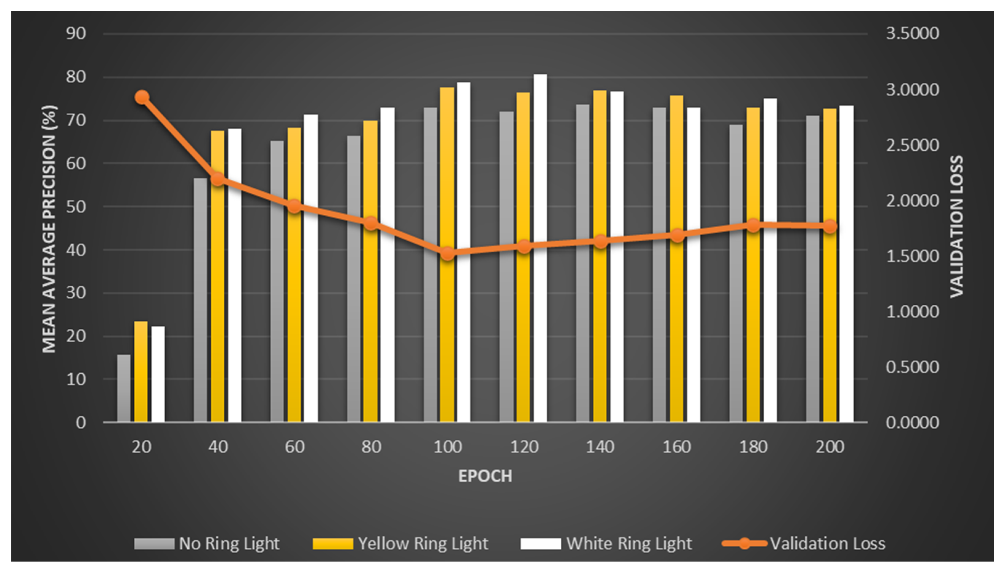
When validating from our table below with 200 epochs on a 20-epoch increment, our best F1 score is 81% using white ring light within 120 epochs.

As shown in

Table 4. Mean average precision table with values using different light sources.

Epoch	Validation Loss	No Ring Light	Yellow Ring Light	White Ring Light
20	2.9333	16%	23%	22%
40	2.2033	57%	68%	68%
60	1.9533	65%	68%	71%
80	1.7967	66%	70%	73%
100	1.5300	73%	78%	79%
120	1.5900	72%	76%	81%
140	1.6400	74%	77%	77%
160	1.6933	73%	76%	73%
180	1.7867	69%	73%	75%
200	1.7700	71%	73%	73%

and Figure 7, the validation loss decreases as the number of epochs increases. However, on a certain level, after the 120th epoch, it is slowly increasing again. This is called overfitting. Overfitting is a typical problem in machine learning, where a model is trained too successfully on the training data, leading to poor performance on new, unforeseen data. Overfitting occurs when a model learns the noise or random fluctuations in the training data rather than the underlying patterns. This leads to a model that fits the training data too closely but cannot generalize to new data. As a result, an overfit model will perform well on the training data but poorly on the test data or real-world data because it has not learned the true relationship between the input features and the output. To avoid this, an effective machine learning model should balance the ability to generalize to new data with the ability to fit the training data well to prevent overfitting. This can be accomplished by applying regularization techniques, simplifying the model, or providing more training data. Additionally, using a dedicated ring light greatly affects our accuracy. When comparing the white and yellow lights, there was a slight difference in detection, and most of the time, the white light gave the highest accuracy percentage. Then, epochs were increased from the usual 100 to 200. This did not improve the overall performance.

However, when the number of epochs was increased to around 120 epochs, the accuracy increased, and the validation loss decreased. After 125 epochs, the performance did not improve. From this result, the code was revised to take the lowest validation loss on a given epoch stream. Below is an example with 200 epochs, but the system uses the lowest validation loss at the 125th epoch (Figure 8).

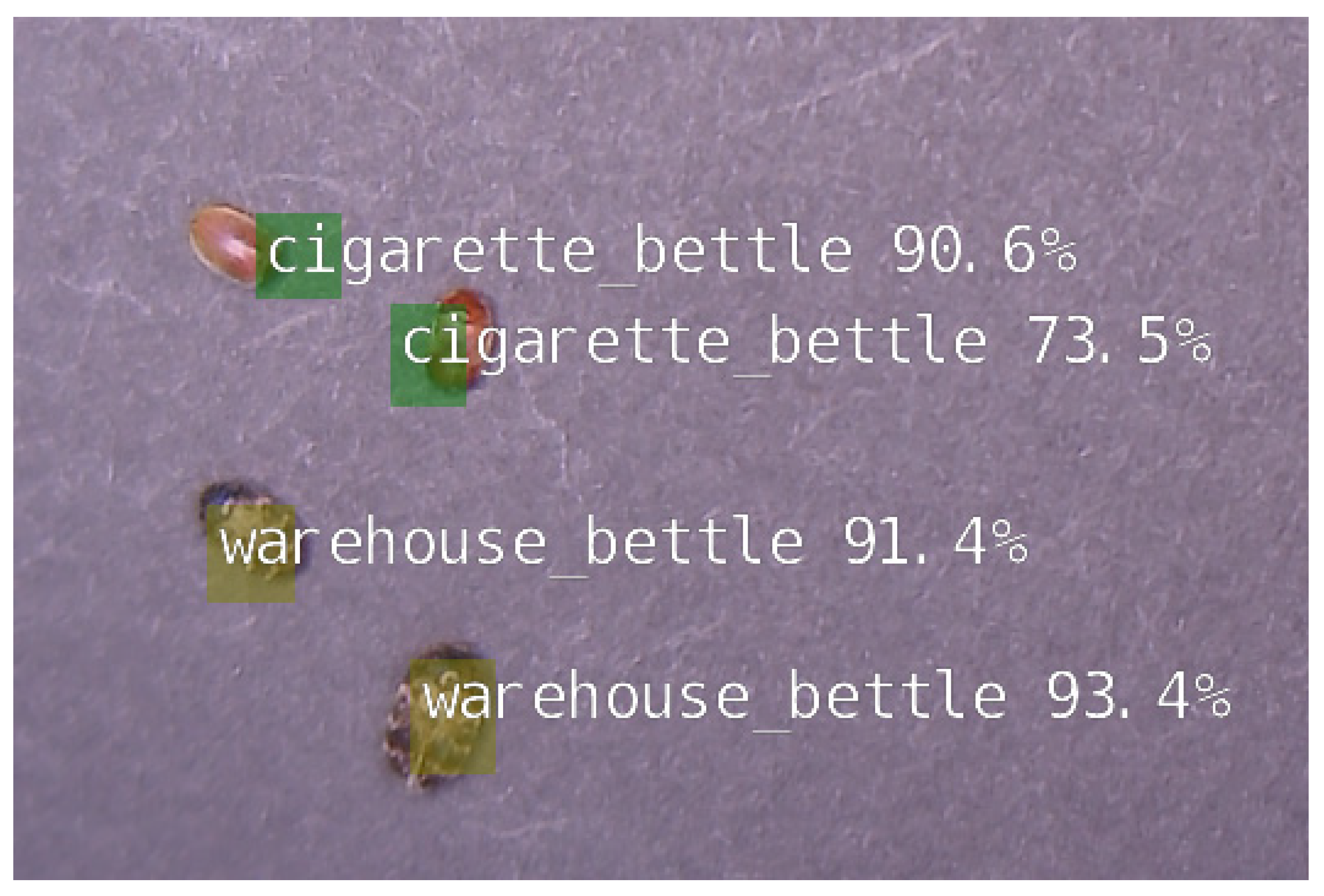
Most published papers regarding insect detection and classification only use one insect per classification, but in this research paper, side-by-side testing was used with smaller-scaled insects. By doing this, a decrease in accuracy was noticed. When detecting and classifying one insect, accuracy is around 85–90% depending on the angle (our camera is in manual focus) and lighting condition. Then, doing it side-by-side, the accuracy is around 70–85% (Figure 9). One of the reasons is because the model is overfit. Increasing our training data set and re-training the model are needed to improve the results. Adjusting the annotation and providing additional spaces on the edges will also help.

4. Conclusions and Future Direction

This study successfully achieved its goal by developing a camera-based monitoring system to detect and identify small-scale insects, using a live feed video for the model to verify, and achieving a confidence level of at least 70% using a side-by-side comparison. There were some difficulties with the lighting and camera set-up since our camera is manual focus, and the total capacity of our designed model was limited. Adjusting the distance of the insects from the camera and manually adjusting the focal length of the camera to focus on the insects was a difficult and tedious task. This is not a reliable concept when applying it to a real-world scenario because, in the real world, insects are crawling and flying. This means losing valuable data while adjusting the settings on the camera since it is out of focus. Another challenge is to address the overfitting by providing additional training data.

Despite these challenges, the results were promising, and we believe the model has the potential for further improvement with the right modifications and technological advancements. To overcome the limitations of manual focus, we plan to integrate an auto-focus camera in the future. This will eliminate the need to manually adjust the camera settings now and then. Additionally, we will gather more diverse and larger data sets to increase the accuracy and robustness of the model. With these improvements, our camera-based monitoring system has the potential to become an effective tool for monitoring and identifying small-scale insects in various industries, such as agriculture and forestry. In conclusion, the camera-based monitoring system showed favorable results, and we believe that with further development, it can become a valuable tool for monitoring and identifying small-scale insects in a range of industries.

The ability of the system to identify insects accurately could lead to more effective pest management practices, reducing the reliance on harmful chemicals and improving crop yields. The system could also be used in environmental monitoring, providing valuable data on insect populations and their potential impacts on ecosystems. The potential applications of this technology are vast and exciting, and we are eager to continue its development and improve its capabilities. The technology could also have applications in areas such as public health by assisting in the early detection and monitoring of disease-carrying insects. It could also provide valuable information for scientific research, aiding in the study of insect behavior and its role in the food chain. Furthermore, the accuracy could greatly benefit farmers and food producers, leading to more efficient and cost-effective crop pest control. This technology can revolutionize how we approach insect detection and management, and its full potential is yet to be explored. It is important to point out that the test cases in this study involved insects that had stark morphological differences. Many insects are almost identical in features, so the technology would need much more refinement, or it could just serve as an initial screening tool for general identification.

Future research on machine vision is expected to investigate other aspects, such as the implications of using auto-focus cameras on image analysis. Performance comparisons of different algorithms are currently being carried out and will be written up in a new paper. Additionally, the impact of clear and blurred images on the analysis accuracy will be another area of focus. Although serving latency was deemed insignificant for two insects, further investigation will explore how it could become more relevant as the number of insects being analyzed rises. These additional factors will contribute to a more comprehensive understanding of the potential and constraints of machine vision in various applications.

For future work, the plan is to incorporate a cloud-based platform for storing and retrieving data for future analysis. Developing a stationary and autonomous mobile platform incorporating processing and communications capabilities to transfer information to a server for additional processing and user output is also on our list, as is implementation in a real-world scenario to help our farmers detect and identify these insects and provide the necessary actions to eliminate the level of infestation on their stored product facilities.