1. Introduction
The Causal Cognitive Architecture 4 (CCA4) is a biologically inspired cognitive architecture that uses spatial navigation maps as its main data elements. These “navigation maps” hold spatial data, just as, for example, an automobile road map holds various roadway-related spatial data; however, the architecture’s navigation maps are also used for holding operations that can be performed on other navigation maps as well as being the substrate where the operations can occur.
A cognitive architecture represents a theory of how a mind works, which is also able to be implemented in some artificial system, usually via a computer simulation. A number of cognitive architectures have been developed in the last few decades [
1,
2,
3]. Biologically inspired cognitive architectures (BICA) tend to be more loosely inspired by biological constraints, often with the goal of creating human-level cognitive functioning. The Causal Cognitive Architecture is a mammalian brain-inspired architecture with regard to certain biological features, rather than trying to duplicate every pathway of the biological brain.
A key biological inspiration of the Causal Cognitive Architecture was the extensive implementation of navigation maps as the main data structures of the system. In the last two decades, research has shown the key role of navigation maps in the hippocampus of the mammalian brain [
4,
5,
6,
7,
8]. Cognitive modeling of spatial navigation has been considered by Langley [
9]. It has been suggested by Schafer and Schiller that both the hippocampus and the neocortex contain maps of spatial items as well as non-spatial items which would include information related to social interactions and more abstract features such as concepts [
10]. Hawkins and coworkers have noted that the grid cells in the hippocampus, which have been shown to contain a representation of the location of the experimental animal in the external world, may also exist in the neocortex, and thus perhaps the entire neocortex can used as a spatial framework in which to store the structure of objects [
11].
Another biological inspiration of the Causal Cognitive Architecture involved offering a model that incorporated the navigation maps mentioned above, and showed how, with relatively few changes (i.e., corresponding to a feasible biological evolutionary path), the Causal Cognitive Architecture’s behavior could change from pre-causal but stable abilities to an architecture capable of full causal behavior, though at a much higher risk of psychotic-like behavior.
Except for humans, most other mammals do not readily demonstrate psychotic symptoms. While other mammals cannot communicate as clearly as humans, it is possible to observe symptoms of many other psychiatric disorders in their behavior at times; however, psychosis is rare. In fact, it is challenging to induce laboratory animals to show schizophrenic-like symptoms for use in psychopharmacological research environments [
12]. On the other hand, greater than 10% of the human population will have psychotic or psychotic-like symptoms at some point [
13]. Similarly, while humans readily can demonstrate full causal behavior, even as infants [
14], other animals even as adults do not show full casual abilities. For example, the Asian elephant has brain of much greater size than a human brain, yet Nissani has shown that the elephant’s behavior occurs as a result of associative learning rather than genuine causal abilities [
15]. For example, (non-mammalian) crows are often portrayed as being able to show full causal behavior, but Neilands and colleagues show that, in experiments (e.g., dropping an object down a tube in order for a food item to become available to the bird), there is actually little causal understanding [
16]. Primates can use a stick to push food rewards through and out of a tube; however, if a gravity trap (i.e., a hole in the tube) is added, there is relatively poor genuine understanding of the actual cause and effect, and associative learning is used to figure out how to shove the food around the hole and through the tube [
17].
An early version of the Causal Cognitive Architecture showed how, by increasing the feedback pathways from the module where operations are performed on the navigation map to the sensory input modules, the architecture went from pre-causal behavior to more fully causal behavior, albeit with the risk of psychotic-like malfunctioning [
18,
19,
20,
21]. The actual mechanism is discussed in more detail in the sections below. The next version of the architecture, named the Causal Cognitive Architecture 1, made much more extensive usage of navigation maps and showed that it was possible to create a system with the potential for intelligent behavior based on navigation maps [
22]. In the Causal Cognitive Architectures 2 and 3, a solution to the binding problem was presented as a necessity so that the architecture could handle non-toy problems without the risks of the combinatorial explosion of processing larger sensory inputs as well as the usual condition in the real world of inputs changing with time [
23,
24]. In these architectures, there was binding of both the features of space and of time onto navigation maps. The actual mechanisms are discussed in more detail in the equations and description below.
Below, we present an enhancement of the Causal Cognitive Architecture in a new Causal Cognitive Architecture 4 (CCA4).
Figure 1 depicts a summary of this architecture. Given that the Causal Cognitive Architecture is (albeit, loosely) mammalian brain-inspired, and given that there is our assumption discussed above that the neocortex is largely functionally composed of navigation maps, now, in the CCA4 the navigation maps for each of the sensory systems which in the CCA3 were stored outside of the main repository of navigation maps within separate Input Sensory Vectors Association Modules, they are more closely integrated with each other and the multisensory navigation maps stored in the Causal Memory Module.
One result of the change is that the CCA4 now more faithfully reflects biological cortical organization, where different sensory modalities have their own regions [
25]. However, a more important result which emerges is that a core processing operation of the Causal Cognitive Architecture 4 now readily and extensively makes use of analogical reasoning. This does not refer to solving analogical problems one would see, for example, on a human intelligence test (although the core analogical reasoning operation would contribute to the solution of such problems), but rather that analogical reasoning is used ubiquitously by the architecture in the processing of most sensory inputs and the solution of most day-to-day problems.
2. Operation of the Causal Cognitive Architecture 4 (CCA4)
In this section, we walk through the operation of the Causal Cognitive Architecture 4 (CCA4). Although we use the architecture of the CCA4 (
Figure 1) in this major
Section 2, we largely consider the functionality present in the Causal Cognitive Architecture 3 [
24]. In the following major
Section 3, we consider how the CCA4, unlike the CCA3, now readily and extensively makes use of analogical reasoning.
A “cognitive cycle” is one cycle of the sensory input data entering the Input Sensory Vectors Shaping Modules, passing through the various modules of the architecture, and sending an output to the Output Vector Association Module and then on to the Output Vector Shaping Module, where it becomes translated into a physical output. Then, in the next cognitive cycle, this repeats again—sensory inputs enter the Input Sensory Vectors Shaping Modules and proceed through the architecture, eventually to the Output Vector Shaping Module, causing a motor (i.e., physical) output. Cognitive cycles are well established in cognitive architectures (e.g., LIDA architecture [
26]), in which the environment is perceived, processing occurs, and then there is an output action. While a simple decision may occur in one cognitive cycle, more sophisticated cognitive abilities are biologically believed to be composed of a number of cognitive cycles.
As will be shown below, in some cognitive cycles, there is no output; instead, the intermediate results produced by the Navigation Module (
Figure 1), where an operation occurred on what is termed the “working navigation map” (which is the navigation map of interest at that moment), are transmitted back to the Input Sensory Vectors Association Modules. In the subsequent cognitive cycle, the actual sensory inputs from the environment are ignored and, instead, the intermediate results stored in the Input Sensory Vectors Association Modules are propagated to the Navigation Module as if they are the sensory inputs. As such, there is further processing of the intermediate results in this new cognitive cycle. This can continue for a number of further cognitive cycles until there is an output transmitted to the Output Vector Association Module to the Output Vector Shaping Module to a real-world motor action. This is shown by Schneider [
19,
20,
21,
22] as a mechanism by which a navigation-based system could evolve with relatively few evolutionary changes from a system with pre-causal abilities to a system with the ability for full causal processing. By feeding back and re-operating on the intermediate results from the Navigation Module (where operations on the navigation map of interest at that moment are occurring), the architecture can formulate and explore different possible causes and effects of actions [
19,
20,
21,
22]. This is discussed below in the description of the CCA4.
2.1. Overview of the Navigation Maps
The “navigation maps” used in the architecture are (arbitrarily sized) 6 × 6 × 6 arrays holding spatial information about what is in the external environment (although this can be, and is, co-opted to represent internal higher-level concepts). As an example, the features
water–line–solid in the (2,3,0), (2,4,0), and (2,5,0) cubes (each cube corresponding to a coordinate) of a navigation map, for example, could be representing part of a river in those similar locations in the external environment. A cube in a navigation map tends to hold more primitive sensory features, rather than the word “water” or the word “solid.” There will be some sort of representation of a primitive sensory feature (which will be some value linking to the sensory feature) in a cube. With regard to more advanced representations, such as, for example, representing the concept of a lake, rather than water, this is discussed in [
19,
22,
24]. In addition, the grounding problem is discussed below. The CCA4 takes a very pragmatic approach to grounding—it is not an absolute requirement that a feature in a cube be grounded; however, when it is not, there are other requirements to be met.
There are additional dimensions to the navigation maps which hold a variety of other information for each navigation map, such as the binding of separate objects in a scene (i.e., sensory scene involving not only visual inputs but also inputs to any other sensory systems such as auditory, tactile, olfactory, and so on) as distinct objects, for example, or operations to perform on a current or other navigation maps, for example. With regard to spatial binding, in the example above, water–line–solid is stored in the (2,3,0), (2,4,0), and (2,5,0) cubes of a navigation map. Perhaps this navigation map has, for example, also the representation of a rock in the (2,3,0) as well as (3,3,0) cubes. The rock features need to be bound as a continuous object distinct from the water, and another dimension of the navigation map is used for that.
In another dimension of a navigation map, there can be operations specified which are to be performed on two cubes or the entire map of the navigation map. For example, if the contents of one cube are greater than the contents of another cube, then the inferior cube’s contents can be deleted to increase contrast. As well, operations can be specified on other navigation maps. For example, an operation can specify to compare two navigation maps for similarity, or, for example, to compare a navigation map to the millions of navigation maps kept in the Causal Memory Module (
Figure 1).
Some navigation maps are more dedicated to performing operations on other navigation maps, and these maps are termed the “instinctive primitives” or the “learned primitives.” Instinctive primitives are navigation maps which are already preprogrammed and are included with a brand-new instantiation of the architecture. For example, there is an instinctive primitive which causes an action for the architecture to change direction away from a body of water, i.e., so that the architecture avoids bodies of water. Learned primitives, on the other hand, are navigation maps which the architecture learns from experience involving operations to perform on other navigation maps.
From
Figure 1, note that certain modules such as the Learned Primitives Module, the Instinctive Primitives Module, as well as the Goal/Emotion Module have a “D” in the box representing the module. The D stands for developmentally sensitive, i.e., as the architecture gains more experience, for example, the type of goal which is activated will become different. Similarly, as the architecture gains more experience, the type of instinctive primitives which become activated for a given circumstance will also be different from the more immature architecture.
As is shown in the sections with the equations below, the input sensory data are also stored in navigation maps of the same dimensions, as with most of the other navigation maps. There are six main types of navigation maps used in the CCA4, the first five types being of the same dimensions, and the first five allowing operations with each other:
Local Navigation Maps (LNM, defined in Equation (14) below);
Multisensory Navigation Maps (NM, defined in Equation (23) below);
Instinctive Primitive Maps (IPM, defined in Equation (23) below);
Learned Primitive Maps (LPM, defined in Equation (23) below);
Purposed Navigation Maps;
Module-Specific Navigation Maps.
The local navigation maps (
LNMs) are navigation maps in each of the different sensory modalities into which incoming sensory data is mapped. In each cognitive cycle, for example, there will be a separate visual
LNM and a separate auditory
LMN created (or re-used). These are mapped and stored within the Input Sensory Vectors Association Modules shown in
Figure 1.
The multisensory navigation maps (
NMs), often simply referred to as navigation maps, have information from various local navigation maps (
LMNs) mapped onto them. For example, in a cognitive cycle, the information in a visual
LMN and the auditory
LMN can then be mapped onto a new or existing
NM, which will thus have both visual and auditory (and other sensory) information mapped onto it. Many millions or billions of navigation maps can be stored within the Causal Memory Module (
Figure 1). The currently activated navigation map (thus, upon which operations can be performed) is termed the ‘working navigation map’ (
WNM).
The instinctive primitive maps
IPMs are navigation maps of the same dimensions as the
LMNs and
NMs. However, they are used more so to direct operations on other navigation maps than to store information about various features from the sensory inputs. The instinctive primitive maps
IPMs are pre-programmed and come with the architecture. The learned primitive maps
LPMs also direct operations on other navigation maps, but these are learned and created by the Navigation Module (
Figure 1) when new operations are performed by the architecture.
The purposed navigation maps include a number of navigation maps derived from navigation maps NM, however, are used for slightly different purposes, generally involving only a small number of maps, unlike navigation maps NMs, which may number in the millions or billions and are stored in the Causal Memory Module. These maps are discussed in the sections below. Some of these navigation maps include:
Vector Navigation Maps (VNM, defined in Equation (48) below)
Audio-Visual Navigation Maps (AVNM, defined in Equation (48) below)
Visual Segmentation Navigation Maps (VSNM, defined in Equation (52) below)
Context Navigation Map (CONTEXT, defined in Equation (57) below)
Working Navigation Map (WNM, defined in Equation (58) below)
The module-specific navigation maps include navigation maps that are slightly different in structure and function than the main navigation maps discussed above. For example, although not fully discussed below, the Sequential/Error Correcting Module’s procedures make use of stored navigation maps that allow the rapid calculation of vector motion through a matching process. For example, although the Output Vector Association Module’s procedures would also seem to be mathematically symbolic, they too make use of stored navigation maps that allow rapid pre-shaping of the output signal. These navigation maps are specialized and stay local to their modules—the navigation map addressing protocol discussed below will not be able to access these specialized, local navigation maps.
2.2. Overview of the CCA4
Sensory data stream in from different sensory system sensors to the Input Sensory Vectors Association Modules, where they are mapped onto the best matching (or new) local navigation maps in each sensory modality. Then, in the Object Segmentation Gateway Module, any objects detected are segmented, i.e., their spatial features are considered as part of one object. In the example above, we described how the rock is considered a single object. While this object is mapped in the three spatial dimensions, in another dimension in the navigation map, the various features of the object are mapped together to indicate that it is a distinct object. Then, the visual, auditory, and other sensory systems’ LNMs (local navigation maps) are mapped onto the best matching (or new) multisensory navigation maps NM from the Causal Memory Module. This newly updated navigation map then becomes the navigation map the architecture is focused on, i.e., the “working navigation map” WNM.
The local navigation maps will trigger navigation maps in the Instinctive Primitives Module and the Learned Primitives Module. A best matching (i.e., to the content of the segmented local navigation maps) instinctive primitive IPM or a best matching learned primitive LPM is chosen and becomes the “working primitive” WPR. The working primitive causes the Navigation Module to perform on the working navigation map the triggered operations specified by the working primitive WPR. For example, perhaps the working navigation map WNM should be compared against maps which exist within the Causal Memory Module and then replaced with another navigation map. The primitives essentially cause small operations to be performed on the working navigation map WNM (and other navigation maps, as they are activated as the current working navigation map). Primitives can be thought of as being similar to productions of other cognitive architectures or as algorithms of more traditional computer systems. However, primitives are themselves part of navigation maps, and primitives operate on other navigation maps.
Just as in the mammalian brain there are extensive feedback pathways throughout the cortical structure, in the CCA4, there are also extensive feedback pathways. The extent of these feedback pathways is only modestly reflected in
Figure 1. Feedback pathways allow the state of a downstream circuit to bias the recognition of upstream sensory inputs. However, in the CCA4, the feedback pathways from the Navigation Module feeding back to the Input Sensory Vectors Association Modules have been enhanced. As such, the working navigation map currently active in the Navigation Module can be fed back and stored temporarily in the Input Sensory Vectors Association Modules. Then, in the next cognitive cycle, the working navigation map is fed back to the Navigation Module, where it will undergo subsequent additional processing. As such, the working navigation map active within the Navigation Module can represent the intermediate results of the processing of particular sensory input information, which can then be processed repeatedly as needed to arrive at the results required by a more complex problem.
In a cognitive cycle, if the sensory inputs are processed by the Input Sensory Vectors Association Modules, then the Object Segmentation Gateway Module, and then the Navigation Module, to result in a working navigation map upon which the operation of a primitive (in every cognitive cycle an instinctive primitive or a learned primitive will automatically operate on the active working navigation map) yields an actionable result (i.e., a result which can be turned into an action), then that action is propagated on to the Output Vector Association Module. Then, the action is propagated on to the Output Vector Shaping Module, and then the action occurs in the real (or simulated) world. Then, a new cognitive cycle begins, processing whatever new sensory inputs are presented to the architecture.
However, if the result of the operation of a primitive on the working navigation map is not actionable, then, instead of propagating an action on to the Output Vector Association Module, the feedback signal (i.e., the working navigation map) from the Navigation Module to the Input Sensory Vectors Association Module is held in the Input Sensory Vectors Association Module, with the cognitive cycle ending without an action. In the following cognitive cycle, the newly sensed sensory data presented to the architecture propagate as before to the various Input Sensory Vectors Association Modules, but they are ignored. Instead, the working navigation map that was stored in the Input Sensory Vectors Association Modules is propagated to the Object Segmentation Gateway Module and to the Navigation Module. Another primitive can now operate on the working navigation map. Thus, this effectively allows multiple operations on intermediate results until an actionable result is obtained.
As noted above, this cognitive architecture provides an evolutionarily plausible mechanism for the rapid evolution from pre-causal primates to fully causal humans. Moreover, as noted above, this mechanism, at the same time, accounts for the negligible risk of psychosis in pre-causal primates to a significant risk of psychotic-like malfunctioning in humans, discussed in more detail by Schneider [
18,
19,
20,
21]. There is a biological basis for the existence of cognitive cycles. Work by Madl and colleagues has estimated human cognitive cycles to occur every 260–390 milliseconds [
26].
2.3. Input Sensory Vectors Shaping Modules
As shown in
Figure 1, Sensory Inputs for sensory modalities 1…n are fed into the Input Sensory Vectors Shaping Modules 1…n. (Note: Due to the multiple types of navigation maps as well as the multidimensional array notation, to reduce confusion of which items “n” is counting, it is replaced by “ϴ_σ”, i.e., ϴ_σ represents the total number of sensory systems (Equation (8)). Since there is one Input Sensory Vectors Shaping Module for each one of the sensory modalities, there thus exists Input Sensory Vectors Shaping Modules 1…ϴ_σ.)
The sensory inputs for any particular sensory modality are detected as a 2D or 3D spatial array of inputs, which vary with time. In the current computer simulation of the CCA4, visual, auditory, and olfactory inputs are simulated. However, the sensory inputs allowed can easily be expanded to additional sensory modalities.
The CCA4 is loosely brain-inspired, and, as such, we have decided not to physiologically more closely model the olfactory sensory pathways as they occur in the actual mammalian brain. Rather, we have treated the olfactory inputs, as well as any future synthetic senses (e.g., a radar or lidar sensory system), in a fashion similar to other senses in the mammalian brain which proceed through the thalamus to the neocortex. Moreover, in the CCA4, we did not model a split left–right brain which occurs in biology. For example, in the brains of mammals, when some object being observed moves from the left to the right visual hemifield, its representation then moves from the right to left cortical hemisphere, as demonstrated in the research of Brincat and colleagues [
27] showing the interhemispheric movement of working memories.
In Equations (1)–(6), we see that the inputs from visual, auditory, olfactory, and other possible sensory systems are stored in various size three-dimensional arrays that vary with time, i.e., with every cognitive cycle, these values change. In Equation (9), the vector s(t) contains the arrays which represent the sensory system inputs Sσ,t of the different sensory systems. It is transformed into a normalized s’(t) (Equation (10)). All sensory system σ inputs S’σ,t now exist in arrays with dimensions (m, n, o, p) (Equation (11)).
Arrays of dimension (
m,
n,
o,
p) will be the common currency of the CCA4. The spatial dimensions are represented by
m,
n, and
o, while
p represents the extra hidden dimensions the navigation map uses to represent segmentation (i.e., which features belong to which objects), to represent actions to be performed, and to store and manipulate metadata.
2.4. Input Sensory Vectors Association Modules
Figure 1 shows that the Input Sensory Vectors Association Modules, the Navigation Module, the Object Segmentation Gateway Module, and the Causal Memory Module are grouped together and are collectively termed here the “Navigation Module Complex”. This complex is loosely inspired by the mammalian neocortex, and it stores and processes navigation maps.
- -
Note that, for each sensory system σ, there is a different Input Sensory Vectors Association Module. Vector s’(t), representing the normalized input sensory data for that cognitive cycle, is propagated from the Input Sensory Vectors Shaping Modules to the Input Sensory Association Modules;
- -
The local navigation map LNM is defined in Equation (14)—it is an array of the same dimensions as the arrays used by all the navigation maps in the architecture. As noted above, a “local” navigation map refers to a navigation map dedicated to one sensory modality. These maps are stored within the Input Sensory Vectors Association Modules. The vector all_mapsσ,t represents all existing LNMs (local navigation maps) stored within a given sensory modality system σ, while LNM(σ,mapno,t) represents the particular LNM with the address mapno (Equation (15));
- -
As shown in Equation (17) array S’σ,t is matched against all the local navigation maps all_mapsσ,t held within the Input Sensory Vectors Association Module σ. For example, the visual system processed inputs S’1,t are matched against all_maps1,t, i.e., all the LNMs (local navigation maps) stored within the visual Input Sensory Vectors Association Module (Equations (15–17)).
- -
WNM’t−1 in Equation (17) refers to the working navigation map which has been fed back from the Navigation Module in the previous cognitive cycle. Normally, this feedback signal is used to bias the matching of the input sensory data. However, as discussed above, in certain cases, the previous working navigation map can be used as the next cognitive cycle’s input and thus effectively intermediate results are re-processed by the navigation module. This is shown below. However, here, in Equation (17), this is not occurring. The downstream WNM’t−1 (derived in a section further below from WNM, which is defined in Equation (58), with both being of the same structure and dimensions) is simply being used to influence the recognition of the upstream sensory inputs;
- -
For reasons of brevity, named procedures are used in several equations in this paper to summarize the transformations of the data. If details of the procedures are not specified, then more details can be found in [
24]. For example, as noted above, in Equation (17), the procedure “match_ best_ local_ navmap” matches the sensory inputs against the stored local navigation maps in a particular sensory system and returns the best-matched local navigation map;
- -
Then, in Equations (20) and (21), the best-matched
LNM(σ, ϓ,
t) (local navigation map) is updated with the actually occurring sensory input
S’σ,t. Note that, if the best-matched local navigation map is very different than the sensory inputs, then, rather than update the best-matched local navigation map, a new local navigation map is created (Equation (21)). The updated local navigation map (Equation (20)) or the new local navigation map (Equation (21)) is stored within the particular sensory system Input Sensory Vectors Association Module. Moreover, it is propagated to the Object Segmentation Gateway Module (
Figure 1);
- -
The vector lnmt (Equation (22)) represents the best-matched and updated actual sensory inputs local navigation maps LNM’(σ, ϓ, t) of all the different sensory systems of the CCA4.
2.5. Navigation Maps
The same array structure of dimensions m × n × o × p forms each of the main types of navigation map. As noted above, there are five main types of navigation maps used in the architecture (and a sixth type of module-specific navigation maps which are not discussed in this section):
Local Navigation Maps (LNM, defined in Equation (14));
Multisensory Navigation Maps (NM, defined in Equation (23));
Instinctive Primitive Maps (IPM, defined in Equation (23));
Learned Primitive Maps (LPM, defined in Equation (23));
Purposed Navigation Maps.
The local navigation maps (
LNMs) were defined above in Equation (14). Local navigation maps (
LNMs) are navigation maps in each of the different sensory modalities in the Input Sensory Vectors Association Modules (
Figure 1). The normalized sensory input vectors feed to the various Input Sensory Vectors Association Modules and are mapped onto local navigation maps (
LNMs). As shown above, in each cognitive cycle, for example, there will be a separate visual
LNM and a separate auditory
LMN created (or re-used).
The multisensory navigation maps (
NMs), often simply referred to as navigation maps, are defined below in Equation (23). As is shown in sections further below, the multisensory navigation maps (
NMs) have information from various local navigation maps (
LMNs) mapped onto them. For example, in a cognitive cycle, the information in the visual
LMN and the auditory
LMN can then be mapped onto a new or existing
NM, which will thus have both visual and auditory (and perhaps other sensory) information mapped onto it. Many millions or billions of navigation maps can be stored in the Causal Memory Module (
Figure 1), where they can be accessed in parallel during search operations. The navigation map, currently activated and upon which operations can be performed, is termed the “working navigation map”
WNM, which has been discussed above and is defined in Equation (58).
The instinctive primitives navigation maps (IPMs) as well as the learned primitive navigation maps (LPMs) are defined below in Equation (23). The instinctive primitives (i.e., instinctive primitive navigation maps), or IPMs, and the learned primitives (i.e., learned primitive navigation maps), or LPMs, are navigation maps of the same dimensions as the LMNs and NMs. However, they are used more so to direct operations on other navigation maps than to store information about various features from the sensory inputs. The instinctive primitive maps are pre-programmed and come with the architecture. The learned primitive maps LPMs also direct operations on the navigation maps somewhat similar to the instinctive primitive maps IPMs, however these are learned and created by the Navigation Module when new operations are performed by the architecture.
all_LNMst (Equation (25)) represents all of the local navigation maps’
LMNs in all of the different sensory systems, i.e., in all the different sensory modules of the Input Sensory Vectors Association Modules (
Figure 1).
all_navmapst (Equation (29)) is simply a representation of all of the different addressable types of the navigation maps in the architecture (i.e., the first four types in the lists above).
Each of the navigation maps (discussed at this point) has a unique address χ given by Equation (32). cubefeaturesχ represents the feature values in a cube (that is, an x,y,z location) in a navigation map anywhere in the architecture at address χ (Equation (35)). cubeactionsχ,t represents the actions in a cube (i.e., x,y,z location) in a navigation map anywhere in the architecture at address χ (Equation (36)). An action is a simple operation that can be performed on a cube in any navigation map, e.g., compare a cube’s value with its neighbor’s value. linkaddressesχ,t represents the linkaddresses in a cube (an x,y,z location) within a navigation map anywhere in the architecture at address χ (Equation (37)). A linkaddress is a link, i.e., a synapse, to another cube in a navigation map or to a cube in a different navigation anywhere else in the architecture. One working navigation map WNM can easily be swapped by another one by following a linkaddress to a new navigation map.
As shown in Equation (38), cubevaluesχ,t represents the contents of any cube (an x, y, z location) in any navigation map (i.e., of the navigation maps discussed at this point), which are all the features, actions, and linkaddresses which may be present in that cube. As shown in Equation (39), this is the same as asking what the value of a particular cube in a particular navigation map is.
The grounding problem asks the question of how the abstract data representations of an artificial intelligence (AI) system can understand the world in which it operates. Harnad [
28] gives an example of a person with no background in Chinese attempting to learn the Chinese language using only a Chinese to Chinese dictionary, whereby the individual ends up going go from one string of Chinese symbols to a different string of Chinese symbols with essentially no meaning being attached by the learner to these symbols. These symbols are said to be “grounded” in yet other different Chinese symbols, thereby, as this example illustrates, providing little meaning to the individual. If any artificial system does not have grounding in the world in which it operates, then the system will have a grounding problem in terms of giving meaning to the system’s internal data structures which it is using to represent the world.
A pragmatic approach is taken by the CCA4 towards the grounding problem. All the occupied (i.e., have contents) cubes contained by a navigation map are required to have at least one grounded feature or, otherwise, at least have a link to another cube anywhere in the architecture, as shown by Equations (41) and (42). Links may go to the low-level sensory features, to a higher-level concept, or to another navigation map. As Harnad points out above, grounding is important. However, the CCA4 also allows navigation maps to consider some features as being grounded via another abstract navigation map. In this manner, the CCA4 can handle representations which essentially act as symbols created during the repeated intermediate results’ processing, and thus not be required to link these representations to some low-level sensory feature, which, at times, would simply not make sense.
2.6. Sequential/Error Correcting Module
While the binding problem is typically thought of in terms of spatial features, i.e., how can the brain bind separately pieces of data [
29], Schneider raises the issue of the need to also bind temporal features [
24]. In the earlier Causal Cognitive Architectures, if features in a navigation map changed, as often occurs with motion, for example, then it became burdensome and complex to process the large volumes of changing navigation maps. However, unlike toy demonstration problems, in most real-world environments, temporal changes are ubiquitous, whether for obvious real-world objects or for higher-level, more abstract concepts, which can also be represented on navigation maps. In fact, mammalian senses generally operate as a function of time. The auditory sensory system detects and represents changes in sounds with respect to time, the tactile senses measure changes in touch with respect to time, and even the visual sensory system’s sensation of a picture which may be static in terms of changes in light with respect to time, as the eyes perform saccadic movements. Thus, in the Causal Cognitive Architecture [
24], it was proposed to bind temporal features as spatial features in the navigation maps by propagating the sensory inputs in a parallel path via the Sequential/Error Correcting Module, as indicated in
Figure 1.
- -
s’_series(t) represents a time series of the recent sensory inputs (Equation (43)). In Equations (44) and (45), the time series of the visual and auditory sensory inputs are represented. The procedure “visual_inputs” (and similarly the procedure “auditory_inputs”) actually does very little since the different sensory inputs are being propagated in parallel to the Sequential/Error Correcting Module. However, in Equations (46) and (47), the procedures “visual_match” and ”aud_match” calculate vectors representing the change in the time of the visual and auditory inputs;
- -
In Equation (48), two new types of navigation maps are defined, one termed a vector navigation map VNM and the other termed an audio-visual navigation map AVNM, both possessing similar dimensions similar to the other navigation maps in the CCA4. Then, the vector navigation map VNM binds the visual sensory motion visual_motion (Equation (49)). Then, the vector navigation map, now termed VNM’, binds, in addition, the auditory changes in auditory_motion (Equation (50)). The resulting vector navigation map VNM’’ thus now contains a spatial representation of the temporal changes in the visual and auditory input sensory data (the current implementation and simulation of the CCA4 does not consider temporal changes in other senses, although they could easily also be included). VNM’’ then propagates to the Object Segmentation Gateway Module, and we examine below how it is bound onto the rest of the input sensory data;
- -
As well as binding the auditory input sensory data along with the visual input sensory data (useful if the architecture needs to function in the real world so the location of sounds can better be handled), the auditory input sensory data undergoes further processing in Equation (51) during the procedure “aud_match_process”, where features of the auditory signal which could be useful to better recognize an incoming sound (as well as allowing recognition of auditory communication) are mapped onto an audio-visual navigation map, AVNM, and are propagated to the Navigation Module complex;
- -
As discussed in the section below, another navigation map, termed the visual segmentation navigation map, VSNM, is defined in Equation (52) but is actually created in the Object Segmentation Gateway Module in an attempt to segment a visual scene into the distinct objects present in the scene. VSNM then propagates into the Sequential/Error Correcting Module, where a time series of VSNMs is created (Equation (53)) and a motion vector visseg_motion is determined (Equation (54)). Then, this motion vector is added as a spatial feature to the current VSNM, which is now termed VSNM’. Thus, VSNM’ is a navigation map containing a visual sensory scene of the spatial features of the segmented (i.e., detected) objects in the incoming visual input data as well as the motion of those objects. VSNM’ then propagates back to the Navigation Module complex.
2.7. Navigation Module Complex: Object Segmentation Gateway Module
The Object Segmentation Gateway Module tries to best take a sensory scene and then segment it into distinct objects. Above, we gave the example of recognizing a rock as a distinct continuous object from the water. In the current embodiment of the architecture, only the visual local sensory map LNM’(1, ϓ, t) is segmented (Equations (56)–(60)). However, it is theoretically possible to segment any of the other sensory modalities.
A visual local sensory map LNM’(1, ϓ, t) is segmented (i.e., recognize distinct objects) by the procedure “visualsegment”, as shown in Equation (60), to yield the visual segment navigation map, or VSNM. Essentially, in the VSNM visual segment navigation map, the extra dimension p of the navigation map is used to hold information defining visual information as distinct objects. In the current simulation of the CCA4, the procedure “visualsegment” simply attempts to match continuous lines with previous objects stored in the visual local sensory LMN maps kept in the visual Input Sensory Vectors Association Module;
Equation (60) shows that, in addition to segmenting visual local navigation map LNM’(1, ϓ, t) into the objects it contains (i.e., adding information to LNM’(1, ϓ, t) which indicates which visual features have been detected as distinct objects), the visual and auditory motion information contained in VNM’’ is applied to VSNM. In addition, there is another parameter, CONTEXT, which can bias the segmentation procedure. In the present implementation of the architecture, it is simply assigned to previous working navigation map WNMt−1 and is not fully used by the architecture at this point;
The visual segment navigation map VSNM thus takes the incoming visual sensory local navigation map LNM’(1, ϓ, t) and adds information indicating which visual features make up distinct objects, as well as any motion information concerning the visual scene and the auditory sensory inputs. The motion information is added to the navigation map as a spatial feature, i.e., as a vector indicating direction and strength of motion;
The motion information VNM’’ refers to visual scene and the auditory sounds as a whole. To further parse out motion information about the individual objects, VSNM is then propagated onto the Sequential/Error Correcting Module, where the visual segment navigation map VSNMt (Equation (60)) is transformed into VSNM’t (Equations (52)–(55)) and then contains visual sensory information segmented into different objects as well as information about the motion for each of these objects. VSNM’ is then propagated to the Navigation Module complex.
2.8. Navigation Module Complex: Causal Memory Module
Now that the single sensory local navigation maps
LMNs have been processed for segmentation (in the case of the visual sensory input data) and motion (in the case of the visual and auditory sensory input data), they are compared with the previously stored multisensory navigation maps stored in the Causal Memory Module. Equation (61) compactly indicates this with the procedure “match_best_navmap”.
Figure 2 shows an overview of how the matching occurs. There is, in this figure, an example of a sensory scene involving a river with water flowing through it and some rocks in the water, including a larger one near the bottom part of the river shown. This is shown on the left side of the figure. The local navigation maps
LMNs created from the input sensory data from this sensory scene are simply indicated as a “Local Visual Navigation Map”, a “Local Olfactory Navigation Map”, and a “Local Auditory Navigation Map”.
On the right side of the figure and to the bottom of the figure are Navigation Maps
NM A to D. These are 6 × 6 × 6 navigation maps
NM; however, we use them as 6 × 6 × 0 two dimensional maps for the purpose of this illustration. Moreover, note that there can be millions or billions of navigation maps
NMs kept within the Causal Memory Module. They will normally have proper addresses, as described in Equation (32) above. We use the letters A to D for the sake of simplicity in
Figure 2;
The visual local navigation map LMN matches best with Navigation Map NM A and Navigation Map NM B of all the navigation maps NMs in the Causal Memory Module. Note that, while a visual local navigation map LMN contains only visual data, the Navigation Maps NM A and B retrieved from the Causal Memory Module are multisensory (i.e., may contain sensory data from any or all of the sensory modalities) navigation maps.
The auditory local navigation map LMN in this example make the best match with Navigation Map NM C and Navigation Map NM A of all the navigation maps NMs in the Causal Memory Module. The olfactory local navigation map LMN makes the best match with Navigation Map NM D of all the navigation maps NMs in the Causal Memory Module.
The procedure “match_best_navmap” (Equation (61)) sees which of these navigation maps match the closest as well as considering matches in more than one sensory system (e.g., Navigation Map A
NM matched for both the visual
LMN and the auditory
LMN). Moreover, in the current implementation, more points are given to visual
LMN matches than the other sensory modalities that exist. In the example in
Figure 2, Navigation Map
NM A is considered to be the best-matched navigation match from the Causal Memory Module. Thus, Navigation Map
NM A becomes the working navigation map
WNM (Equation (61));
The working navigation map
WNM at this point represents the best stored multisensory navigation map which matched against the different sensory modality local navigation maps constructed from the input sensory data. This is done because the input sensory data may often be incomplete, and, as such, a more detailed navigation map can be used via the matching and retrieving of a stored navigation map. This is discussed in more detail in [
24].
The next step is to update the working navigation map WNM (which at this point is a matched navigation map taken from the Causal Memory Module) with the actual sensory inputs that occurred. actualt (Equation (63)) is a vector representing the processed sensory inputs: VSNM’t containing objects and motion from the visual sensory inputs, AVNMt containing audio information from the auditory sensory inputs, and LNM’(3, ϓ, t) containing information from the olfactory sensory inputs. The current implementation of the CCA4 uses visual, auditory, and olfactory input senses; however, as noted above, additional sensory modalities can easily be added. WNMt is then updated with the current sensory input and transformed into WNM’t (Equations (65) and (66)). If the differences between the current input sensory data and the matched WNM are small, then WNM will be updated (Equation (65)). However, if there are too many differences, then, instead of using the matched working navigation map WNM, there will be a new navigation map used to map the current sensory inputs (Equation (66)). Future work may allow a combination of Equations (65) and (66), depending on the novelty of actualt compared to the matched navigation map NM;
An example of updating the working navigation map
WNM and transforming it into
WNM’t (Equations (65) and (66)) is shown in
Figure 3. On the left side of the page is the actual sensory scene. On the right side of the page is the working navigation map
WNM, which is the best-matched navigation map
NM A. The terms “olfactory”, “auditory”, and “visual” represent spatial and temporal features of the sensory scene, i.e.,
actualt (Equation (63)). These features are mapped onto the navigation map
WNM. Thus, note that
WNM now shows the motion of object moving in the direction of the vector mapped onto the navigation map. Note also that
WNM now shows lines representing the larger rock in the river. This updated version of
WNM is now termed the working navigation map
WNM’, which the next sections below process.
2.9. Navigation Module Complex: Navigation Module
As noted above, some navigation maps are actually more dedicated to performing operations on other navigation maps, and these maps are termed “learned primitives” and “instinctive primitives.” Primitives can be thought of as being similar to productions of other cognitive architectures or as algorithms of more traditional computer systems. However, primitives are themselves part of navigation maps, and primitives operate on other navigation maps.
Equations (72) and (74) show that the Learned Primitives Module and Instinctive Primitives Module receive the input sensory data as well as signals from the Goal/Emotion Module and the Autonomic Module. In each cognitive cycle, at least one instinctive primitive will always be triggered by the incoming sensory data and signals from the Goal/Emotion Module and the Autonomic Module.
In the current implementation, if analogical reasoning is not used to select the best primitive (similar to way analogical reasoning is used below to process intermediate results (Equations (86)–(91)), the procedure “match_best_primitive” (Equations (72) and (74)) scores the various primitives triggered according to how strong the match was with the incoming sensory data and signals from the Goal/Emotion Module and the Autonomic Module;
In the current implement, if a learned primitive is triggered (often, it will not be, as the store of learned primitives may be very limited when the architecture is new), then it is used as the working primitive WPR. Otherwise, the triggered instinctive primitive is used as the working primitive WPR (Equations (76) and (77));
Thus, in each cognitive cycle, there will always be a working primitive WPR which can operate on the working navigation map WNM’. In Equation (78), the procedure “apply_primitive” applies the working primitive WPR on the working navigation map WNM’ and produces an action which is the output of the Navigation Module. The action vector should be distinguished from the definition of action in Equation (33), where an action is a simple operation that can be potentially performed on a particular (or multiple) cube (i.e., x, y, z location) within a navigation map. For example, if an agent using the architecture is moving towards a body of water, and there is an instinctive primitive to avoid water, then, in this example, the action output could, for example, be to change direction;
If the action vector produced contains the word or equivalent for “move”, then this is a valid output, and it will be propagated to the Sequential/Error Correcting Module and the Output Vector Association Module (
Figure 1) (Equation (80)). The procedure “motion_correction” will adjust the output motion for the existing motions of the objects in a scene (Equation (82)). Then, the Output Vector Association Module will apply this output motion correction and build up an
output_vector’ (Equation (83)) which specifies in more detail what motions are expected from the agent using the architecture.
output_vector’ is propagated onwards to the Output Vector Shaping Module. This module directly controls the actuators producing the output action;
If the action vector produced does not contain the word or equivalent for “move”, then this is not an actionable output. As Equation (84) shows, in such a case, the working navigation map WNM’ will instead be sent back to the Input Sensory Vectors Association Modules. In the next cognitive cycle, the Input Sensory Vectors Association Modules will automatically treat these intermediate results as if they are LMNs of new sensory inputs and automatically propagate them to the Navigation Module complex (Equation (85)).
There can be repeated processing of the intermediate results of the Navigation Module, as shown in Equations (84) and (85). Once an actionable result is reached, then the
action can be propagated to the output modules, and, in the next cognitive cycle, new sensory input data can be considered. However, if, despite the repeated processing of the intermediate results, no actionable
action is produced, then
WPR can force termination (i.e.,
WPR outputs a signal containing the word or equivalent for “discard”) (Equations (84) and (85)). Similarly, even if processing a working navigation map produces an actionable
action (i.e., it contains the word “action” or equivalent), there may be circumstances where
WPR still wants the results processed again in the next cognitive cycle, and it will contain the word “feedback” or equivalent (Equations (84) and (85)).
3. Analogical Reasoning in the CCA4
Previously, we went through an overview of the functioning of the Causal Cognitive Architecture 4 (CCA4), largely considering the functionality already present within the older Causal Cognitive Architecture 3 (CCA3) [
24]. In this major
Section 3, we now consider how the CCA4, unlike the CCA3, readily and extensively makes use of analogical reasoning, not to solve specialized analogy human intelligence tests, for example, but rather as a core mechanism of the architecture.
3.1. The Problem of Toy Problems
A toy problem is a simplified problem that removes the many complexities of the real world so that research work can focus on what are thought to be the main challenges and allow researchers to give more concise and exact solutions [
30]. Unfortunately, while solutions to toy problems may appear close to a solution of the real-world problem which would seem to simply require a scaling up of the toy problem solution, often this is not the case;
The Causal Cognitive Architecture 1 (CCA1), involving many of the same characteristics shown in the CCA4 above, demonstrated the use of navigation maps to produce pre-causal behavior. Then, when the feedback pathways from the Navigation Module back to the Input Sensory Vectors Associations Modules were enhanced to enable re-processing of the Navigation Module’s intermediate results (similar to Equations (84) and (85) above), it was able to demonstrate full causal behavior [
22]. For example,
Figure 4 shows a gridworld forest where the architecture (i.e., the CCA1) is to direct an agent to find the lost hiker in the forest. The architecture does not have the information of
Figure 4 but must build up an internal map of the external world, which it is starting to do in
Figure 5. If the CCA1 moves to the square “forest” just north of the “wtrfall” (waterfall) square, it needs to make a decision about its next move. It has an instinctive primitive that avoids deep bodies of water and thus inhibiting it from moving west to the square “lake.” It has already explored the northeast and thus wants to explore south now to look for the lost hiker. It is able to cross rivers (no instinctive primitives are activated by rivers) and so it moves to the square “wtrfall” with fast moving but shallow water. Unfortunately, the fast-moving water sweeps it over the cliff of the waterfall, and it becomes damaged, thus failing at its mission;
If a brand new CCA1 architecture/agent (if the previous one is used, it will now have an associative memory not to enter fast-moving rivers) is now in the same situation, but full feedback (i.e., similar to Equations (84, 85)) is active, then there is more advantageous causal behavior. The new CCA1 architecture/agent has not encountered a waterfall previously. However, {“flowing fast” + “noise”} + {“water”} will trigger inside the Instinctive Primitives Module the primitive {“push”}. Then, the Navigation Module transmits {“push”} + {“water”} back to the Input Sensory Vectors Association Modules, where it is used as the input for the next cognitive cycle. {“water”} + {“push”}, when re-processed, triggers an instinctive primitive which retrieves a navigation map of where the CCA1 is being pushed under water. This is re-processed in the next cognitive cycle and triggers an instinctive primitive to stay away and change direction. Thus, the new CCA1 architecture/agent changes direction and moves east to the square “forest” and avoids the “wtrfall” square.
The CCA1 was able to show that a system of navigation maps could produce intelligent, causal behavior, albeit on toy problems. Thus, it was thought that, perhaps by programming a larger repertoire of instinctive primitives, tweaking some algorithms, and improving the implementation, that the CCA1 could truly start solving more challenging real-world problems. However, it soon became clear that, in the architecture of the CCA1 (which is different than the CCA4 architecture shown in
Figure 1), there was an issue in fusing together input sensory features. As the sensory environment became even slightly larger compared to the toy environment of the gridworld with the lost hiker, there developed a combinatorial explosion of the complexity needed for the processed vector which was transmitted to the Navigation Module. To overcome this issue, the Causal Cognitive Architecture 2 (CCA2) was designed, wherein sensory inputs are bound onto navigation maps, rather than produce a signal to send to the Navigation Module for later processing [
23,
24].
The spatial binding solution of the CCA2 seemed to work well on toy problems and also on some larger problems that started approaching real-world problems. However, the CCA2 only worked well if the problems and the world was static. Once there was a change in motion or a change in the environment, a massive number of navigation maps needed to be processed for even small problems (e.g., 30 navigation maps per second times 10 s was 300 full navigation maps to process and make sense of versus a single navigation map for static problems);
In most real-world environments, changes in time are ubiquitous. To overcome this issue, the Causal Cognitive Architecture 3 (CCA3) was created, where sensory inputs are also bound for temporal features [
24]. Binding was done in a spatial fashion (e.g., Equations (49) and (50) above). Thus, instead of 300 full navigation maps of a changing world being used to process in the example above, there was only the need to process a single navigation map with time and space bound onto the navigation map;
The solution provided by the CCA3 seemed to overcome previous problems and seemed to more genuinely offer the hope that, if the system was made more robust (e.g., create a larger library of instinctive primitives, improve some algorithms, improve the implementation), then it would be able to handle real-world problems with intelligent causal behavior. However, it soon became apparent that creating a large enough library of instinctive primitives to deal with the many challenges of environments even modestly larger than a toy environment was challenging. Unlike the toy example above of avoiding the waterfall in the gridworld, for many problems slightly more advanced, the CCA3 simply was not able to activate the instinctive primitives that would even be useful for the problem at hand, even if the intermediate results were re-processed hundreds of times.
3.2. The Causal Cognitive Architecture 4 (CCA4)
As noted earlier, in the CCA4 the local navigation maps
LMNs for each of the sensory systems, which in the CCA3, were stored outside of the main repository of navigation maps in separate Input Sensory Vectors Association Modules, are still stored in separate Input Sensory Vectors Association Modules, though they are now more closely integrated with each other and the multisensory navigation maps within the Causal Memory Module (
Figure 1). This more faithfully reflects biological cortical organization, where different sensory modalities have their own regions [
25]. However, given the ease of feedback and feedforward pathways in this arrangement, with another circuit coopted as a temporary memory, analogical reasoning emerges from the architecture.
In keeping with biological evolution, Equations (84) and (85) are duplicated and modified using a slightly different pathway through the circuits. Equations (84) and (85) are still valid if the working primitive WPR contains the signal “feedback.” In this case, as before, the working navigation map WNM’ is fed back to the Input Sensory Vectors Association Module (Equation (84b)). In the next cognitive cycle, this working navigation map WNM’ is then fed forward (by co-opting the LMNs from the actual sensory inputs, as before) to the Navigation Map (Equation (85b)), and there is processing again, possibly by a different working primitive WPR. Thus, if specified by the working primitive WPR (Equation (84b)), then this capability to re-process intermediate results, as such, still exists in the CCA4.
However, in the CCA4, the newer duplicated and modified feedback pathways (Equations (86)–(91)) are now used as the default option for the re-processing of intermediate results. As before, if the operation of the working primitive WPR on the working navigation map WNM’<x> does not result in an actionable output, i.e., actiont does not contain the signal “move”, then the procedure “feedback_store_wnm” propagates the working navigation map WNM’<x> back through the feedback pathways to temporarily be stored in the Input Sensory Vectors Association Modules (Equation (87))—this is the same as before. (Please note that the angle brackets in Equations (87)–(91) have no effect on the variables—they are simply there to help the reader follow the Humean induction by analogy that is occurring. Thus, WNM’<x> has the same meaning as WNM’, other than pointing out to the reader that the values in WNM’ at this point represent x in the induction that is occurring.)
In Equation (86), a temporary navigation map tempmem has been defined. Unlike other long term storage navigation maps NM being saved within the Causal Memory Module or the long term storage local navigation maps LMN being saved long-term in their respective Input Sensory Vectors Association Modules, tempmem is a navigation map in which the Navigation Module can store a navigation map temporarily and then easily read it back. In Equation (88), we see that the working navigation map WNM’<x> is also compared with the navigation maps in the Causal Memory Module, with the best-matched navigation map being copied to tempmem<x>.
The procedure “next_map1” in Equation (89) looks at the most recently used linkaddress (Equation (37)) for the working navigation map tempmem<x>. The navigation map to which WNM’<x> (or related navigation map tempmem<x> if the best matching in Equation (88) resulted in a slightly different navigation map) most recently linked to now becomes WNM’<y> (Equation (89)). As noted above, the angle brackets have no special meaning other than to help the reader follow the induction by analogy that is occurring.
In Equation (90), the working navigation map WNM’<y> subtracts the navigation map in tempmem<x>, with the result going to a new working navigation map WNM’<B>.
Then, in the next cognitive cycle, the original working navigation map WNM’<x> that was stored within the Input Sensory Vectors Association Modules is propagated back to the Navigation Module; however, instead of overwriting the current (i.e., active) working navigation map WNM’<B>, the “retrieve_and_add_intermediates” procedure causes this retrieved WNM’<x> to be added to the existing working navigation map WNM’<B> (Equation (91)). We can call this new working navigation map WNM’<x+B>. As noted above, the angle brackets have no special meaning other than to help the reader follow the induction by analogy that is occurring.
Note that this very automatic mechanism has essentially stored into WNM’<x+B> (i.e., the current version of WNM’ at the completion of Equation (91)) the action that occurred in the past of a similar working navigation map in a situation that may possibly be analogical. This analogical processing of the intermediate results often will produce an actionable output when processed by the working primitive WPR. If not, the working primitive WPR can feed back the result present in the navigation module for analogical re-processing again in the next cognitive cycle, or for the previously described conventional re-processing, again in the next cognitive cycle, or it can discard the intermediate results and process new actual sensory inputs in the next cognitive cycle. A demonstration example is given in the next section.
From a neuroscience point of view, note that essentially WNM’<x> is being propagated along an additional pathway—to the Input Sensory Vectors Association Modules, as before (Equation (87)), as well as to the Causal Memory Module (Equation (88)). The subtracting of two navigation maps in Equation (90) and the adding of two navigation maps in Equation (91) can easily be done by neural circuits.
From an argument by analogy point of view, consider the following. In Equation (92), we state that navigation map
x has properties
A1,
A2, …,
An. In Equation (93), we state that navigation map
y has properties
A1,
A2, …,
An. In Equation (94), we state that navigation map
y also has property
B. Therefore, in Equation (95), we conclude, by induction by analogy, that navigation map
x also has property
B. In Equation (91), the working navigation map
WNM t’<x+B> now also has property B.
4. CCA4 Demonstration Example
Results from the run of a computer simulation of the Causal Cognitive Architecture 4 (CCA4) are presented below. While navigation maps in the implementation of the simulation are spatially 6 × 6 × 6; here they are used in a 6 × 6 × 0 mode which allows easier display and printing of results.
The Abstraction and Reasoning Corpus (ARC) is a collection of analogies that uses visual-only grids with colored boxes [
31]. There are usually two to four solved training instances of how one visual grid should be transformed into another one. Then, there is a test example. The ARC examples only depend on basic innate knowledge a person would largely have about objects. The examples do not depend on human experiences of the world and stories humans are familiar with.
As a test example for the CCA4, a simplified visual scene is taken from the ARC. However, we do not allow any immediate training, but rather assume that the CCA4 architecture being used has seen the versions of somewhat similar training examples in the past. In real life, events do not happen as neatly as they do in analogy intelligence tests. Thus, it is closer to a zero-shot test of learning, rather than the few-shot learning in the ARC. In the test example below, the visual scene involves areas of water on a piece of otherwise featureless landscape. There is no particular human meaning attached to this visual scene. Indeed, a human would find it hard to suggest how this scene should be transformed.
The visual scene propagates through the CCA4 architecture, and the working navigation map
WNM’<x> shown in
Figure 6 is in the Navigation Module. The incoming sensory data or this navigation map does not cause the triggering of any particular primitives, nor actually any particular instinctive primitives. As a result, a default instinctive primitive is triggered so that the working primitive
WPR contains the signal “analogical”.
No actionable output is produced, i.e., action
t ≠ “move*”; rather, the working primitive
WPRt = [“analogical*”]. Thus, as shown in Equation (87), the current navigation map
WNM’<x> is fed back and saved within the Input Sensory Vectors Association Modules.
WNM’<x> is also fed into the Causal Memory Module, where a best-matching navigation map is found. The match will usually return a navigation map very similar to
WNM’<x>, and while it would seem this step is not needed, a stored navigation map is more likely to have different experiences than the present one has had, since there was already a difficulty in processing the working navigation map. The best-matched navigation map is then stored in the temporary memory
tempmem<x> (Equation (88)).
Figure 7 shows an output of the simulation run at this point.
Then, the most recently used
linkaddress in
tempmem<x> accesses the navigation map that it links to and is stored as the new working navigation map
WNM’<y> (Equation (89)).
Figure 8 shows
WNM’<y>, which represents the navigation map which occurred after the best matched
WNM’<x> working navigation map in the past and retrieved again now.
Then,
WNM’<x> working navigation map subtracts the value of
tempmem<x> from itself (Equation (90)). As shown in
Figure 9, this difference,
WNM’<B>, essentially represents the property ‘
B’ that
y possesses in the definition of analogy (Equation (94)). By induction by analogy,
WNM’<x> should also then possess this property. Thus, in Equation (91), the working navigation map
WNM’<x>, being saved in the Input Sensory Vectors Association Modules, is added (as opposed to overwriting, as usually happens) to the current working navigation map
WNM’<B>. The result is the new working navigation map
WNM’<x+B>, as shown in
Figure 10.
Equation (91) occurs in a new cognitive cycle, and a new (or possibly the previous) working primitive WPR will be operating on the current working navigation map WNMt’<x+B>. Possibly, in this cycle, the squares with water are treated by the working primitive WPR, for example, as a body of water, and, for example, the action output, as directed by the WPR, is to change direction away from this body of water, for example.
While, in the Abstraction and Reasoning Corpus (ARC), the purpose of the output is simply to give an answer to an intelligence test, in the CCA4, with limited instinctive primitives, where the concept of intelligence test is not understood, the actions will be more like the example given above, e.g., change direction. However, with sufficient instinctive and learned primitives, the action output could be more appropriate for a test setting.
This example is simplified from the Abstraction and Reasoning Corpus. In order to solve even the full easy analogies in the ARC test set, the CCA4 would require a larger collection of instinctive primitives to deal with objects, geometrical relationships, and object physics. The core analogical mechanism of the CCA4, i.e., Equations (86)–(91), is not intended as a human or machine intelligence test analogy solver. While this mechanism can assist in the solution of human or machine intelligence test analogies, along with a more robust set of instinctive and learned primitives, its purpose is as a low-level mechanism that helps the Navigation Module produce more useful action outputs.
5. Discussion
5.1. A Navigation Map-Based AI—The Causal Cognitive Architecture 4 (CCA4)
Artificial neural networks (ANNs) can perform reinforcement learning and recognize patterns at a human-like level of skill [
32,
33]; however, they perform inferiorly compared to a child in terms of causal problem solving [
14]. The Causal Cognitive Architecture 3 (CCA3) seemed to be able to allow causal problem solving [
24], particularly for simple toy problems. However, for even slightly more complex problems where there were no instinctive or learned primitives exactly fine-tuned for the problem at hand, the CCA3 failed to readily produce useful
action outputs.
Above, we have shown that the architecture of the CCA3 readily allows the addition of small modifications to the architecture, in keeping with its intention to be evolutionarily feasible, forming the Causal Cognitive Architecture 4 (CCA4). In the CCA4, there can occur the production of analogous intermediate results in response to the feedback of the Navigation Module when there is a failure to produce useful
action outputs. Analogous intermediate results fed back to the Navigation Module may not always yield a useful result. The working primitive
WPR must be applied to these results; moreover, sometimes, the intermediate results are not suitable to form the output signal, but, instead, the results are fed back again for re-processing in the next cognitive cycle, either by analogous processing again or by the normal feedback processing present in the previous CCA3 architecture. However, in many cases, the analogous intermediate results do in fact allow a useful
action output to occur, as in the case of the example in
Figure 6,
Figure 7,
Figure 8,
Figure 9 and
Figure 10 above.
As noted above, the analogous processing of feedback results from the Navigation Module in the CCA4 is not intended to be a human or machine intelligence test analogy solver. Rather, analogical reasoning is used ubiquitously by the architecture in the intermediate processing of sensory inputs to solve day-to-day problems the architecture is encountering.
Logically, most of the times when the architecture is unsure of producing a reasonable output in the Navigation Module and feeds back the intermediate results so that they can be re-processed in the next cognitive cycle, inductive reasoning is required. While this reasoning with time can become more statistical, details of the environment typically tend to change so that the Humean component is essential. The analogical intermediate results feedback mechanism (Equations (86)–(91)) used in the CCA4 incorporates both. The instinctive and learned primitives essentially give the laws of environment or universe required by Humean induction. However, the triggering of primitives can become statistical with experience, and the analogical mechanism is essentially reflecting what happened before in other, closely related cases. As noted above, an advantage of the CCA3 was that, by feeding back and re-operating on the Navigation Module’s intermediate results, the architecture can formulate and explore different possible causes and effects of actions [
19,
20,
21,
22,
23,
24]. The analogical reasoning mechanism in the CCA4 further enhances the ability of the architecture to formulate and explore different possible causes and effects of actions in an attempt to produce an advantageous output signal.
5.2. Biological Insights—The Possible Ubiquity of Analogical Reasoning
Given that the CCA4 is a biologically/brain-inspired cognitive architecture (BICA), if the emergence of analogical reasoning as a core mechanism appears to be possible with a few changes as the CCA4 shows, it would suggest that analogical reasoning could have easily evolved and formed a core mechanism in human thought. Rather than considering analogical reasoning as a special ability that humans use when taking intelligence tests, analogical reasoning may be ubiquitous in all our behaviors.
In fact, there has been much psychological evidence supporting analogical reasoning as a core mechanism in human thought. Infants only thirteen months old are shown to make use of analogy as an innate skill [
34]. Hofstadter has argued strongly for the constant use of analogies by the mind for everyday routines tasks [
35]. While solving analogical problems would appear to be a very conscious activity, functional magnetic resonance imaging (fMRI) shows that, in subjects noting similarities between a past event and a new present analogous event, this often occurs unconsciously [
36].
With regard to the evolution of analogical reasoning in the mammalian brain, there is much evidence that, while full analogical reasoning may be restricted to humans (and to some limited extent possibly by other primates [
37]), other animals are able to perform many but not all of the steps required to achieve to full analogical reasoning. For example, Herrnstein [
38] noted the ability of nonhumans to demonstrate four (discrimination of stimuli, categorization by rote, open-ended categories, allowing a range of variation and noting similarity giving the ability to form concepts) out of five (fuller relations between concepts) steps necessary to form abstract relations. Krawczyk [
39] reviewed areas of the brain, particularly certain regions in the prefrontal cortex, involved in human relational thinking and analogical reasoning. Work by Vendetti and Bunge [
40] has shown that relatively small changes in the human brain, particularly the strengthening of connections in the lateral frontoparietal network (a key region related to relational thinking functionality), compared to other primates, can possibly explain the large changes in the ability of humans to perform more powerful abstract relational thinking, including analogical reasoning, compared to other primates.
5.3. Improvements to the Different Learning Systems in the CCA4—Future Work
Learning, of course, is key to any cognitive architecture, as well as any biological brain. The different navigation maps used by the Causal Cognitive Architecture 4 (CCA4) were presented above in
Section 2.5. All these navigation maps use slightly different learning mechanisms. Generally, continual learning is possible for most aspects of the CCA4, just as it is generally possible for most aspects of biological brains. Changing one navigation map generally does not affect the entire network of navigation maps except for some of the updated links. In continual learning, a cognitive architecture or an artificial intelligence should be able to learn new information without causing substantial damage to its existing information. Note that this is not the case for most deep neural networks, where modifying the network on the fly can cause a catastrophic forgetting of learned information.
At present, the learning mechanisms implemented by the computer simulation of the CCA4 (discussed above for the demonstration example) for the different navigation maps are as simple as necessary in order to be in compliance with the equations above and to allow the demonstration examples to run. Future work is planned to enhance these learning algorithms. Below, in
Table 1, we briefly review the learning mechanisms for the main navigation maps presented above in
Section 2.5 and review future work to improve these mechanisms.
With regard to the future work of adding elements of artificial neural networks to some of the navigation map types, the simulation code is written in the Python language and has been interfaced to the PyTorch machine learning framework. Use of conventional neural networks will limit full continual learning; however, wake/sleep cycles have already been implemented into the code; moreover, during sleep periods, there are opportunities for the re-training of any conventional neural networks associated with particular types or individual navigation maps. If conventional neural network implementation can be used on an individual navigation map basis, i.e., using a different neural network for every single navigation map, then re-training requirements are greatly reduced.
Above, in
Section 2.1, there is an overview of the many types of navigation maps used in the Causal Cognitive Architecture 4. The “module-specific navigation maps” are the array structures that are used by various modules for specific local purposes—the navigation map addressing protocol discussed above will not be able to access these specialized, local navigation maps. An example discussed above was the set of module-specific navigation maps used by the Output Vector Association Module. As noted, although the Output Vector Association Module’s procedures would seem to be mathematically symbolic, they too make use of stored navigation maps that allow for the rapid pre-shaping of the output signal. Thus, these module-specific navigation maps also require learning mechanisms. At present, for the toy problems involved in the current simulation, many of these learning mechanisms have been implemented to be as symbolically and programmatically simple as required to be in compliance with the equations above. However, future work, of course, will also consider associating conventional neural networks with these specialized navigation maps to allow more robust learning.
Very specialized module-specific navigation maps also form the array structures that pre-process the sensory input information in the Input Sensory Vectors Shaping Modules. Again, for the toy problems, as well as the use of simulated sensory inputs in the current simulation, many of these learning mechanisms have been implemented to be as symbolically and programmatically simple as required to be in compliance with the equations above. However, future work, of course, will also consider associating conventional neural networks with these specialized navigation maps to allow, in the case of the specialized module-specific navigation maps used for input data, not only more robust learning, but more robust transformation of the sensory inputs.
5.4. Navigating and Benchmarking the Physical World—Future Work
At the time of writing, the computer simulation of the CCA4 utilizes simulated sensory inputs. As noted from the previous section, the result of considering toy problems in conjunction with the simulated sensory inputs more easily allowed the development of the architecture and its computer simulation. However, given that the main inspiration behind this biologically inspired cognitive architecture is the role of navigation maps in the hippocampal structures of the mammalian brain which allows mammals to move about and successfully navigate their environments [
4,
5,
6,
7,
8], it begs the question of how well the Causal Cognitive Architecture can actually navigate its physical world.
Work has begun on the Causal Cognitive Architecture 5 (CCA5) simulation program. Some of the implemented learning mechanisms are being enhanced, as discussed in the above section. In particular, work has started on enhancing the collection of instinctive primitives. In order for the architecture to be able to better control an agent and navigate in the real world, many additional and more robust intuitive physics primitives and intuitive logic primitives are required. The inspiration for these instinctive primitives is biological again. The works of Spelke and others [
41,
42,
43,
44] has shown that an infant’s brain is not a tabula rasa, but rather contains an innate store of knowledge. This knowledge is quite domain specific. For example, infants may perceive shadows, but they do not contain innate knowledge about shadows. However, as Spelke [
42] notes, within the group of innate physics knowledge, infants possess an innate knowledge, for example, that an object will affect another object’s motion only if the objects touch. Kinzler and Spelke [
43] organize this innate knowledge into five groupings and note that parts of it also apply to nonhuman infants:
Objects
- -
cohesion (motion of an object is as a connected whole)
- -
continuity of motion on a path
- -
contact between objects
Agents
- -
motion of agents, unlike objects, for example, do not expect a continuous motion
- -
agents expected to interact with other agents
Number
- -
can apply to different objects/agents, even if they are sensed differently
- -
can compare number representations, even adding and subtracting
- -
number representations become less precise the larger the numbers involved
Geometry
- -
distance, angle, relations between surfaces
- -
orientation with geometry
Us vs. Them
- -
reasoning about social group members
There is an extensive literature on autonomous navigation in the fields of robotics and artificial intelligence [
45,
46]. There is also considerable work in the area of cognitive architectures and spatial navigation [
9,
47]. While navigation in any system may come down to the physics of objects, the behavior of agents, and geometric considerations, the reality is that the mechanisms used by the Causal Cognitive Architecture are quite distinct from most other approaches to autonomous navigation. The Causal Cognitive Architecture will not be able to adequately navigate a real-world environment until a sufficient repository of instinctive primitives are developed as well as enhancements to the learning mechanisms for the array structures that pre-process the sensory input information in the Input Sensory Vectors Shaping Modules discussed in the above section.
As a first step towards real-world navigation, work has begun on the Causal Cognitive Architecture 5 (CCA5) simulation program to augment the instinctive primitives that will be most useful for navigational activities. Moreover, the CCA5 simulation program now automatically detects the presence of a standalone embedded computer board that allows sensor inputs and actuator outputs to potential commercial mobile robot platforms. Arbitrary real-world navigation test environments can be set up. A Causal Cognitive Architecture-controlled mobile robot achieving navigation skills in the real world offers an excellent opportunity for better experimentation with the architecture, including the benchmarking of different versions of the architecture operating in the test navigation environments.
5.5. Navigating and Benchmarking the Abstract World—Future Work
As noted in the section above, the mechanisms used by the Causal Cognitive Architecture are quite distinct from most other approaches to autonomous navigation. A drawback of the Causal Cognitive Architecture is that an adequate set of instinctive primitives must be developed before the architecture can even approach the most minimal real world navigation tasks. However, on the positive side, the architecture offers core causal and analogical processing. Stimuli which it has not seen before can be processed by the application of the instinctive primitives to the navigation map representing the input sensory data. In addition, the architecture can navigate not only the physical world, but the abstract world as well, using the same mechanisms.
As noted above, Schafer and Schiller suggest that both the hippocampus and the neocortex contain maps of spatial items as well as non-spatial items including more abstract features such as concepts [
10]. In the demonstration example above, the CCA4 is presented with an abstract input it has not seen before, yet it attempts to provide a response to the input, in this case, by analogical reasoning. The demonstration example is taken from a simplified example from Chollet’s Abstraction and Reasoning Corpus (ARC) of analogy problems [
31]. As the Causal Cognitive Architecture further is developed, it is proposed to use Chollet’s corpus as a quantitative benchmark of the performance of the architecture.


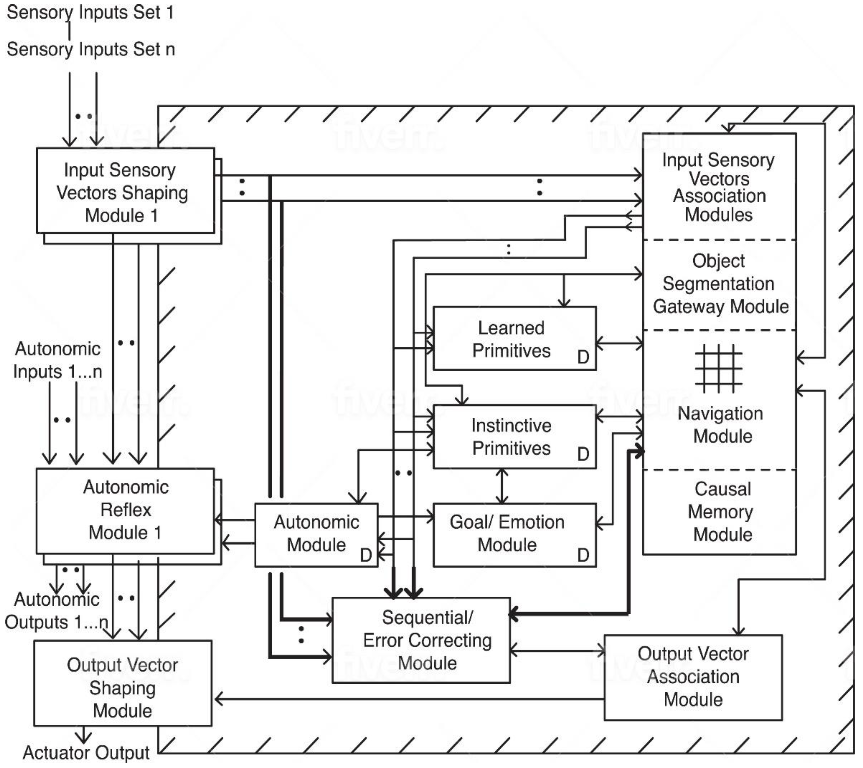

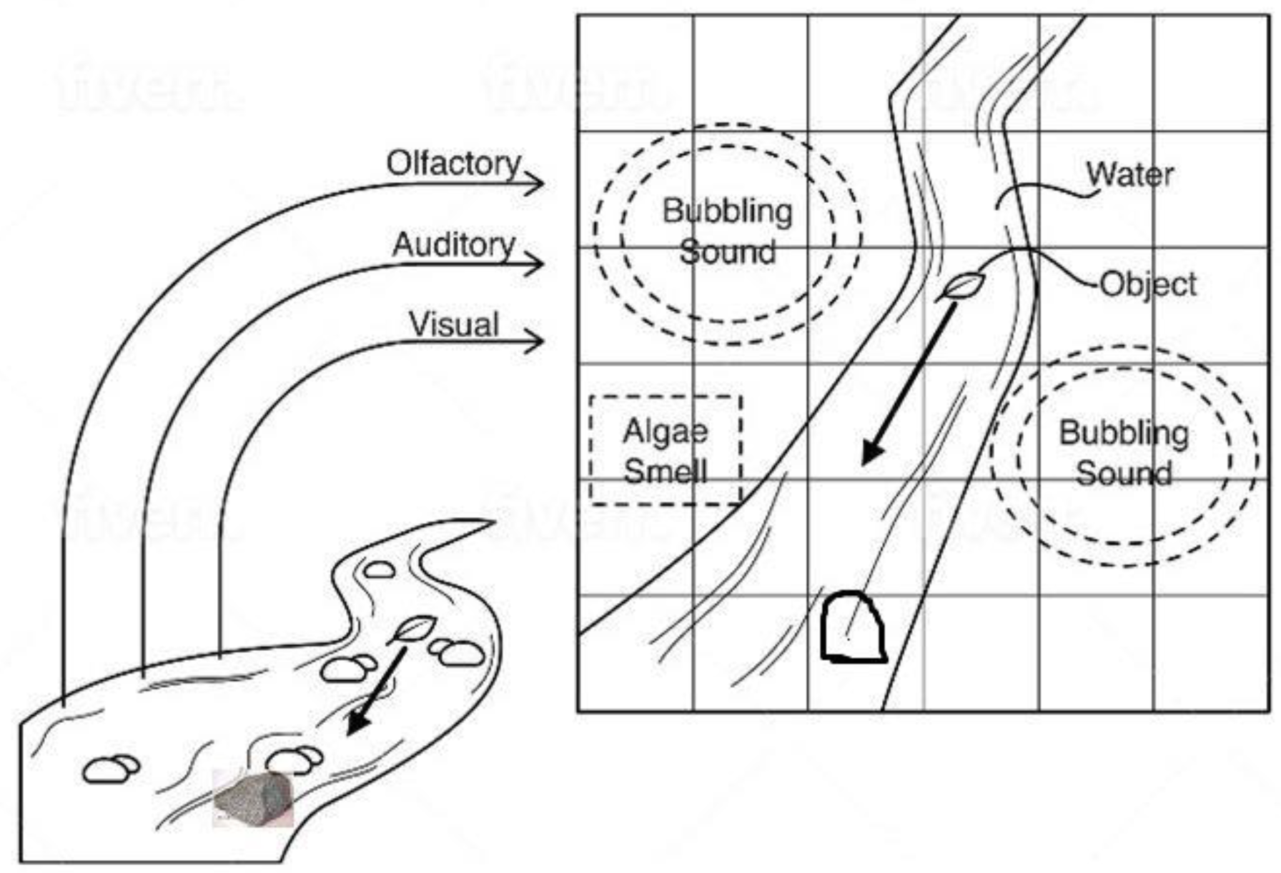


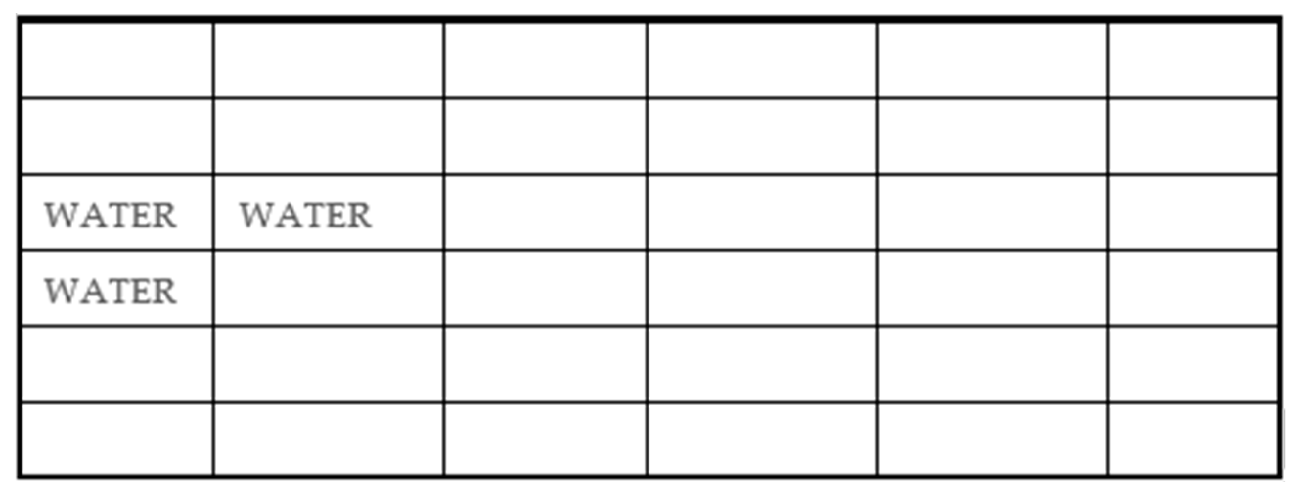

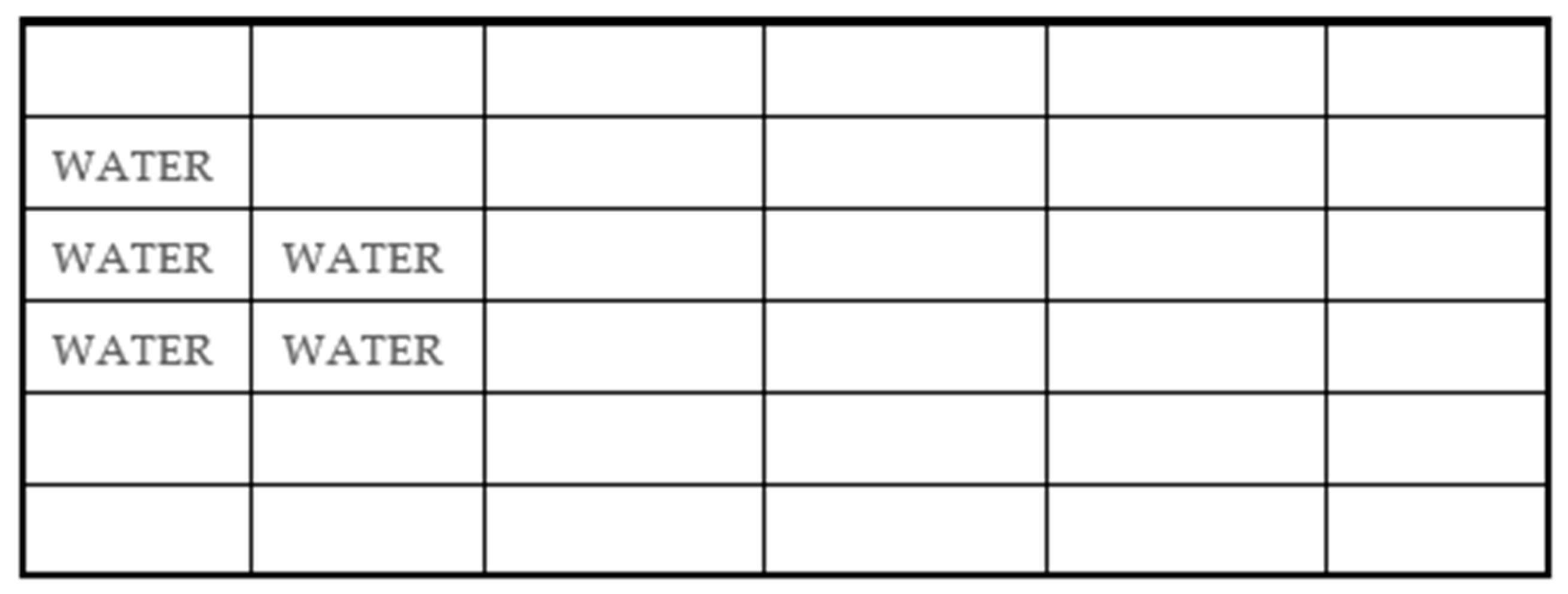
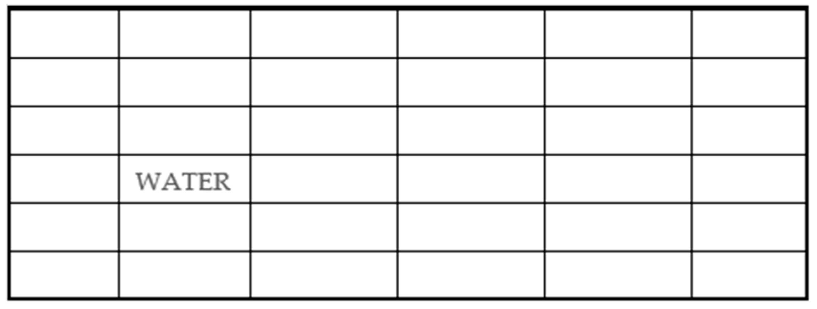


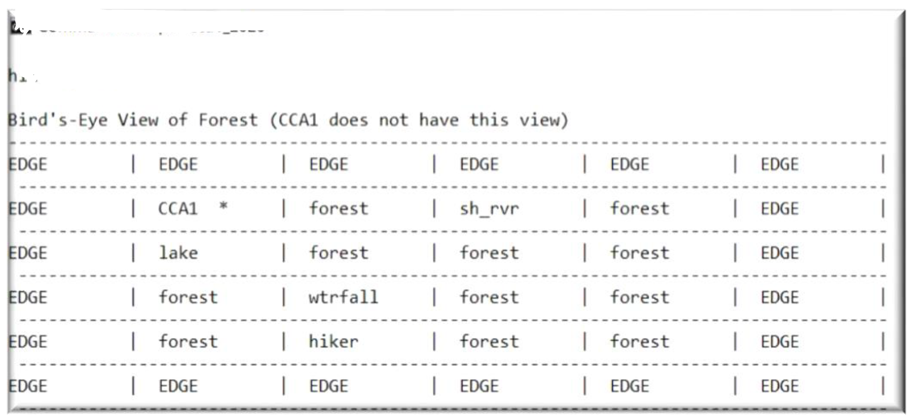
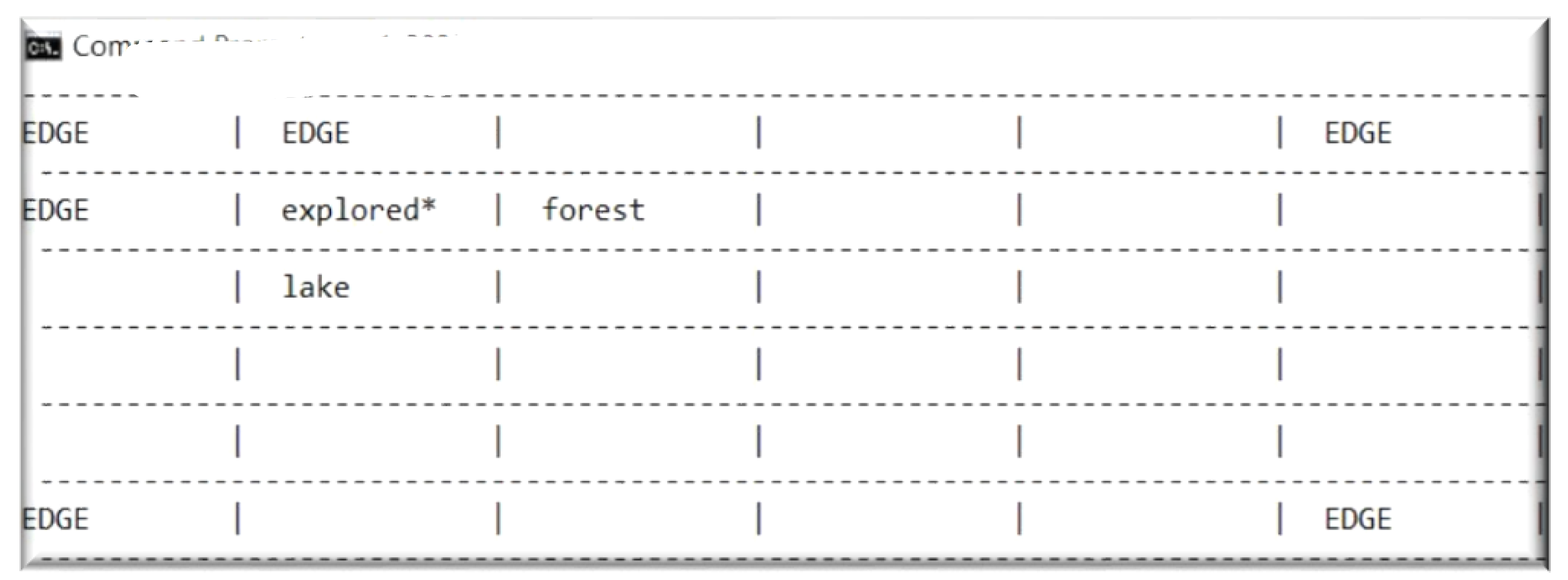
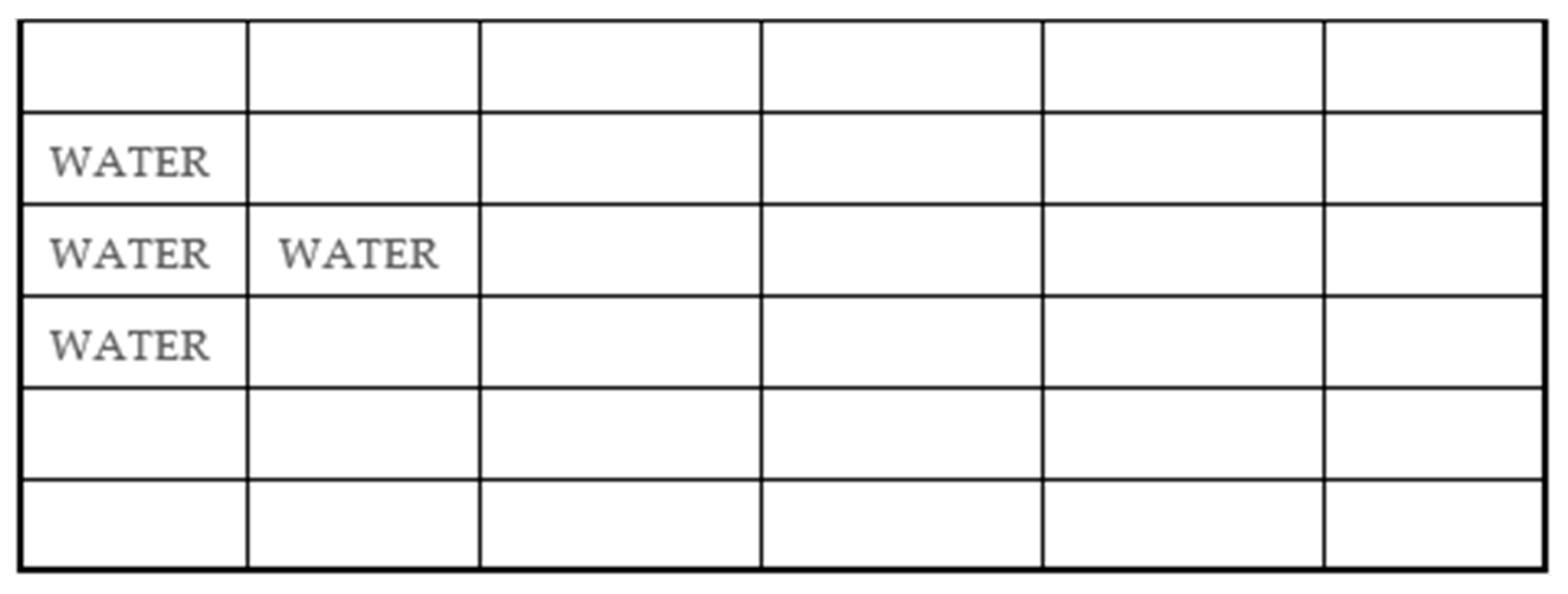
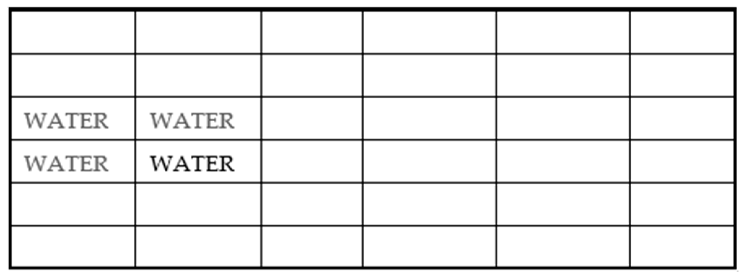