A Particle Swarm Optimization Backtracking Technique Inspired by Science-Fiction Time Travel

Abstract

Artificial intelligence techniques, such as particle swarm optimization, are used to solve problems throughout society. Optimization, in particular, seeks to identify the best possible decision within a search space. Problematically, particle swarm optimization will sometimes have particles that become trapped inside local minima, preventing them from identifying a global optimal solution. As a solution to this issue, this paper proposes a science-fiction inspired enhancement of particle swarm optimization where an impactful iteration is identified and the algorithm is rerun from this point, with a change made to the swarm. The proposed technique is tested using multiple variations on several different functions representing optimization problems and several standard test functions used to test various particle swarm optimization techniques.

1. Introduction

Artificial intelligence techniques draw inspiration from many different sources. One common source for inspiration is from nature. Techniques have been inspired by insects, such as the artificial bee colony algorithm [1], the firefly algorithm [2], and ant colony optimization [3]. Other techniques have been inspired by birds, such as cuckoo search [4] and migrating birds optimization [5]. Particle swarm optimization (PSO) is also inspired by birds [6].

These techniques have found use in numerous problem domains. PSO, for example, has been demonstrated to be effective for antenna design, biomedical applications, communication network optimization, classification and control problems, engine design and optimization, fault diagnosis, forecasting, signal processing, power system control, and robotics [7]. Zhang, Wang, and Ji [8], in fact, reviewed nearly 350 papers on particular swarm optimization and identified over 25 variants of the technique, which found use in ten broad categories ranging from communications to civil engineering.

There are many different sources that can be used for inspiration other than nature. This paper presents a new technique that is inspired by the science fiction concept of time travel. Time travel is a common plot element used in science fiction where a person travels to a different point in time. Time travel can be used to answer complex questions; however, it is only hypothetical and can be, more practically, a source of inspiration. The technique proposed in this paper uses the concept of time travel by returning to an impactful moment in PSO and makes alterations.

The proposed time-travel inspired technique is an enhancement of PSO. PSO is a heuristic method used to solve complex optimization problems that cannot be solved easily with standard mathematical methods. One issue with PSO is that it oftentimes finds solutions that are not the globally best solution for a given search space. This happens when a particle gets trapped in a local minimum and leads other particles to this suboptimal solution. Another issue is the use of time and computational resources. Enhancements to the base PSO technique attempt to solve these issues. Examples include center PSO [9], chaotic PSO [10], and the hybrid genetic algorithm and PSO [11]. Center PSO adds a particle to the center of the search space. This particle does not have a velocity and is used only for calculating the velocity of other particles. The center particle is useful because it increases efficiency for the common case of the optimum being near the center of the search space. Chaotic PSO adds the addition of chaos to traditional PSO. This allows for the algorithm to avoid local maxima. The hybrid Genetic Algorithm and PSO attempts to combine PSO with a genetic algorithm to utilize the benefits of both algorithms.

The technique presented in this paper is a potential solution to the issue of being trapped in local minima. The algorithm can be broken down into eight steps, which are explained in detail in Section 3. It begins by running the PSO algorithm, but not completing the run. The second step is to calculate the most impactful iteration of the run. The third step is to copy the swarm at this iteration. The algorithm continues, in the fourth step, by terminating the particle swarm run. The fifth step of the algorithm is to make an alteration to the copied swarm. The sixth step is to begin a new particle swarm run with the copied swarm. The seventh step is to end this run. Finally, the results of the two runs are compared and the better of the two solutions is chosen. In addition to use with the base PSO algorithm, this technique has the potential to also enhance variations of PSO. This could be achieved by running a new enhancement of PSO, instead of regular PSO, for the first and sixth steps of the algorithm.

This technique aims to change PSO to avoid finding suboptimal solutions. It is expected to find better solutions at the expense of using more computing resources. This paper explores multiple methods of implementing the proposed technique. Two methods for finding impactful iterations are discussed. Multiple changes to the particle swarm, at the impactful iteration, are also discussed. The experiment, outlined in Section 4, assesses the efficacy of combinations of four different change technique variations and two different impact calculation variations of the proposed technique for different complex functions representing optimization problems and several benchmark functions.

This paper continues with background information on related topics–such as artificial intelligence, science fiction, time travel, and PSO–being discussed in Section 2. The proposed technique is described in Section 3 and the experimental design is reviewed in Section 4. Data are presented and analyzed in Section 5 (related to several problem domain applications) and Section 6 (related to common PSO evaluation functions). Finally, the conclusions and potential areas for future work are discussed in Section 7.

2. Background

In this section, background information and related prior work for the proposed technique are presented. First, prior work on and problems that can be solved using artificial intelligence are discussed in Section 2.1. Next, prior work related to swarm intelligence is presented in Section 2.2. PSO is discussed in Section 2.3 and the section concludes with a brief overview of science-fiction time travel literature being presented in Section 2.4.

2.1. Artificial Intelligence and Applications

Countless problems can be solved using traditional procedural programming approaches; however, there are many problems that cannot be solved efficiently in this way. Artificial intelligence approaches have been created for challenges such as the traveling salesman problem [12] (using genetic algorithms, the nearest neighbor algorithm, ant colony optimization, and neuro-fuzzy techniques [13]), computer vision [14] (using neural networks [15] and convolutional neural networks [16]), decision-making [17] (using techniques such as expert systems [18] and the Blackboard Architecture [19]), and complex optimization problems [20].

Artificial intelligence is utilized in many different fields. In medicine [21], it has been used for drug development, disease diagnostics, the analysis of health plans, health monitoring, digital consultation, surgical treatment, managing medical data, and personalized medical treatment. In transportation [22], it has been used for planning, making road construction decisions, improving public transport, traffic sensor operations, and commanding self-driving cars. In law [23], it has been used to automate legal tasks such as filtering discovery documents, allowing lawyers to search through thousands of documents that they would not have time to search manually. It has also been used to automate contract development and predict legal outcomes. In education [24], AI has been used to develop intelligent tutoring systems, which adapt to students’ feedback, and personalized learning capabilities. It has also been used to track students’ performance and educational data, using data mining, to predict potential failure to facilitate intervention. AI, of course, is also utilized in numerous other fields including mental healthcare [25], ophthalmology [26], and industrial marketing management [27].

2.2. Swarm Intelligence

Swarm intelligence techniques, many inspired by insects’ and other animals’ behavior, have also been created to solve problems [28]. Popular insect-based techniques include ant colony optimization [29], which is frequently used for path finding and has also been demonstrated for managing peer-to-peer interconnections in a grid computing environment [30]. Another technique, artificial bee colonies [31], simulates bee colonies by using groups of simulated bees with different roles which work together to iteratively find improved solutions to a problem.

An animal-based technique, spider monkey optimization [32], uses monkeys’ foraging behavior as inspiration. Spider monkeys forage for food in small groups and split into multiple groups when having difficulty locating food, while still collaborating while dispersed. Yet other swarm intelligence techniques are metaheuristic algorithms which are well suited to and employed for solving “sophisticated … optimization problems” [33]. Forestiero [34], for example, demonstrated the use of a neural-concept-based multi-agent system that was employed to analyze “activity footprints” to tackle the complex task of detecting anomalies in internet-of-things devices.

2.3. Particle Swarm Optimization

PSO is also a metaheuristic algorithm and swarm intelligence method that is typically used to solve complex optimization problems [35]. One such problem is the optimal mixing of ingredients to grow useful microorganisms [36]. Another example is using PSO to support or replace backpropagation for neural networks [37,38]. Other applications include its use for Bluetooth and electrical networks, temperature control, and motor design [7]. It has also been used for disease diagnosis, optimizing equipment placement, clustering, and combinatorial optimization [7], in addition to numerous other areas [8].

Domains of its use include [8] electrical, mechanical, chemical, biomedical, and civil engineering, controlling automated systems, communications, and operations management. Key examples [7] of its use include antenna design, designing and improving communications networks, engine and motor design and control, fault detection and recovery, and image analysis. In power systems engineering [39], it has been used for optimization dispatch, reactive control, loss reduction, flow control, and controller design. In robotics [40], it has been used to create collaborative swarm-style techniques for robotic search operations. In finance, PSO’s efficacy has been demonstrated for portfolio optimization [41]. In geotechnical engineering [42], it has been used for analyzing the stability of slopes, “pile and foundation design”, determining rock and soil characteristics and making decisions regarding tunneling operations.

PSO has also been shown to be able to integrate, support, and enhance other AI techniques. Grimaldi, et al. [43], for example, showed that it can be used as an approach for neural network learning processes. Liu, et al. [44] demonstrated its efficacy for supporting big data analysis.

Numerous applications for PSO have been identified. Sedighizadeh and Masehian [45] identified nearly 1800 uses for this style of algorithm across numerous areas. There are also numerous PSO technique variants–Sedighizadeh and Masehian [45] identified approximately 60 categories of PSO techniques, that were classified into areas based on criteria such as the technique’s “fuzziness”, “velocity type”, “recursively”, and “combinatoriality”.

PSO uses a collection of particles [35] that move around in a search space containing the bounds of the function it is trying to optimize. This allows them to search for an optimal solution by iteratively improving their current solutions. Each particle has its own velocity specifying how much distance it will move in the next iteration. This velocity is updated each iteration based on a number of factors. PSO does not always find the global best solution because it can get trapped in local solutions or can take an unrealistic time to converge fully.

2.3.1. Particle Swarm Optimization Variants

A wide number of variants of PSO algorithms have been proposed—Sedighizadeh and Masehian [45] identified 60 categories of PSO algorithms. Many of the variants include combinations with other AI techniques, while others are optimizations of or changes to the base technique. Kashyap and Parhi [46], for example, paired PSO with a proportional integral derivative controller and increased a humanoid robot’s gait performance through increasing the speed of stabilization and reducing “overshoot” by about a fourth. Fan, et al. [47] proposed a “random reselection” technique, based on the Cuckoo search technique, and demonstrated its efficacy for optimizing solar cell systems to provide renewable energy. Ceylan [48] showed how PSO could be applied to “grey modeling”. The PSO grey modeling approach outperformed unaugmented grey modeling, “grey rolling modeling”, and NARNN modeling for predicting the spread of COVID-19 cases.

Kan, et al. [49] proposed the use of an “adaptive particle swarm optimization convolutional neural network” for securing internet-of-things devices. The technique was shown to outperform other techniques–including support vector machines, feedforward neural networks, and convolutional neural networks–in terms of both accuracy and precision. Zaman and Gharehchopogh [50], similarly, combined PSO and a backtracking search optimization algorithm to produce a technique that outperformed other PSO and metaheuristic algorithms in terms of convergency, accuracy, and exploration capability. Li, et al. [51] proposed combining PSO with a grey seasonal model, which was used to predict changes in natural gas production and demand in China.

2.3.2. Particle Swarm Optimization Techniques Advances

The number of PSO advances are too numerous to fully explore herein. Houssein, et al. [52] identified over 300 papers that they associated with “major advances” in PSO and multiple topological categorizations for them. Several recent advances are illustrative of the types of approaches being taken.

Han, et al. [53], for example, proposed the use of “adaptive strategies” in PSO’s feature selection process and demonstrated enhanced performance, in terms of solution optimality, convergence, and diversity, as compared to six other algorithms across 20 datasets with a notable benefit in data with high dimensionality.

Gu, et al. [54] enhanced PSO with the use of surrogate assistance. They used the random forest algorithm with PSO and tested the technique using benchmark knapsack problems. The technique was shown to offer benefits in terms of convergence speed, accuracy, and computational cost. Ji, et al. [55] also used surrogates for multimodal optimization problems. They proposed a dual surrogate design that seeks several optimal solutions. It was shown to compare favorably with both existing surrogate and existing multimodal evolutionary algorithms, in terms of both solution accuracy and computational performance.

Li, Xue, and Zhang [56] proposed the use of a new feature selection algorithm and revised initialization and search space reduction approaches for PSO. A “stick binary PSO” algorithm is used for feature selection, initialization is based on “mutual information”, and a “dynamic bits” search space reduction strategy was implemented. With these enhancements, the technique outperformed eight other techniques that it was compared to. It generated higher accuracy, in many cases, and reduced features in “most” instances.

Sedighizadeh, et al. [57] proposed a new “generalized” PSO algorithm. This algorithm added two additional variables to the velocity equation and also introduced a dynamic update algorithm for particles’ inertia. The proposed technique was compared to multiple other PSO techniques, using key benchmark functions, and generally outperformed the other techniques in terms of runtimes and accuracy.

Liu, et al. [58] proposed a PSO technique that trains a neural network as a way to avoid convergence speed and calculation costs of traditional PSO algorithms. The combined fuzzy neural network and PSO technique outperformed both component approaches, in terms of computational speed, while all three were able to consistently find optimal solutions.

Song, et al. [59] also proposed a hybrid approach, combining three techniques to enhance the process of feature selection. This approach combined filtering, feature clustering, and evolutionary algorithm methods and used an “improved integer PSO” technique to produce a suitable set of features while minimizing processing time requirements.

Wang, Zhang, and Zhou [60] developed a PSO algorithm for problems that require the consideration of both continuous and discrete variables. This approach featured a “mixed-variable encoding scheme” and an adaptive approach to parameter setting. It was found to converge faster and produce more accurate results, while having competitive performance to four other multi-variable techniques it was compared to.

Song, Zhang, Gong, and Sun [61] demonstrated a bare-bones PSO technique that used “mutual information” for the problem of feature selection. It optimized the initialization process and introduced two additional mechanisms for search. The approach was compared to eleven other algorithms and was shown to find a better set of features than the other algorithms, while also having superior computational performance.

Domain-related advancements have also been studied, extensively, in regards to applications such as warehouse operations [62], geotechnical applications [63], financial portfolios and stock trends [64], and disease identification [65].

2.4. Science Fiction and Time Travel

Science fiction has multiple subgenres and themes, including dystopia [66], space [67], and time travel. It has been a source of inspiration for many. It has been used as a way to model the future [68], with prototypes that can be used to compare multiple possible futures to determine how technologies could contribute to the development of society [68]. Science fiction prototyping is a conceptual form of prototyping rather than a physical one [69], which is used to present new perspectives on future technology.

Time travel is a well-known genre of science fiction. However, there is considerable debate about the possibility of time travel because it challenges known principles of physics and presents paradoxes [70].

Despite this, it is commonly used in the literature to hypothesize about abstract questions, such as how past actions impact the present and future. Different perspectives on this exist. Some believe that changes will have pronounced impacts, such as the “butterfly effect” described in H.G. Well’s Time Machine [71]. Others project less impact, such as in Issac Assimov’s What if [72]. Speculating about these questions serves as a source of inspiration in different fields. One example of this is a method for future-oriented user research [73], which can inspire designers and consumers using themes taken from time travel. The artificial-intelligence technique presented in this paper also draws upon the science-fiction genre of time travel as its inspiration.

3. Technique Description

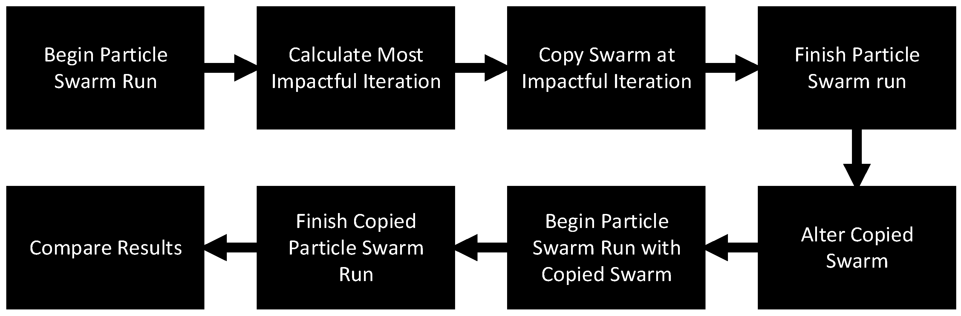
The technique proposed herein is an enhancement of PSO. The technique is split into eight sections, for easier understanding, which are now discussed. These are also depicted in Figure 1. The first step is to begin a particle swarm run. The second step is to calculate the most impactful iteration of this run. The third step is to make a copy of the swarm at the impactful iteration. The fourth step is to terminate the particle swarm run. The fifth step is to make a change to the copied particle swarm from step three. The sixth step is to begin a new particle swarm run with the copied particle swarm. The seventh step is to terminate this particle swarm run. The final step is to compare the results of the two particle-swarm runs and choose the better result.

3.1. First Step: Particle Swarm Run Initiation

The process starts by initiating a particle swarm run. The proposed technique was tested with the base particle swarm optimization algorithm; however, it could be easily adapted for use with other PSO techniques. One minor variation, when implementing PSO, is the velocity update formula. Although many studies use the original formula, others include small changes. The original velocity update formula is [74]:

v_i+1 = (v_i) + (c₁ * r₁ * (p_i − x_i)) + (c₂ * r₂ * (g_i − x_i))

(1)

In this formula, bolded letters symbolize a vector containing an element for each dimension. Scalar terms are not bolded. The vector v_i+1 contains the velocity for the particle for the next iteration. The vector v_i contains the velocity of the particle in the current iteration. The constants, c₁ and c₂, are weights affecting the influence of the particle’s best position and the swarm’s best position, respectively, on the new velocity. The variables r₁ and r₂ are pseudorandom numbers generated between zero (inclusively) and one (exclusively). The vectors p_i and g_i are the particle’s best recorded position and the swarm’s best recorded position, respectively. Finally, the vector x_i denotes the particles’ position at the current iteration.

A minor adaptation of this velocity update formula includes another added constant as its only change. The added constant is denoted by the letter w. This constant is called the inertia weight and impacts the influence of the velocity at the current iteration. The rest of the terms are denoted the same. This updated formula is [75]:

v_i+1 = (w * v_i) + (c₁ * r₁ * (p_i − x_i)) + (c₂ * r₂ * (g_i − x_i))

(2)

The velocity update equation for the proposed technique is a minor adaptation. The only change from this formula to the one used for the proposed technique is the removal of both stochastic variables. The removal of these variables was done to simplify the formula slightly and add less randomness to the environment. This allows for fewer variables changing the results of the proposed technique. The formula used for the proposed technique is shown here with all terms denoted the same as previously:

v_i+1 = (w * v_i) + (c₁ * (p_i − x_i)) + (c₂ * (g_i − x_i))

(3)

The particle swarm was initialized with ten particles. The particles begin in random locations of the search space. The swarm is then run for 100 iterations. The results of this run are saved for the purpose of comparing them to the second particle swarm run.

3.2. Step Two: Impactful Iteration Identification

The second step of the proposed technique is to calculate the most impactful iteration. This step begins during the first particle swarm run. This particle swarm run will terminate before the third step. To determine the most impactful iteration, a numerical variable for determining impact was used. This variable was defined as the extent to which a particle was influenced by other particles in one iteration. Impact was calculated for each particle separately using the equation:

m_i = g_i − x_i

(4)

Here, m_i identifies the impact at the current iteration, g_i represents the global best position of the swarm, and x_i represents the current position of the particle. This formula was derived from the definition included in the previous paragraph. The only point in the algorithm where a particle is impacted by other particles is during the velocity update. The only part of this equation containing effects from other particles during the current iteration is the third term: c₂ * (g_i − x_i).

There are two other terms of the equation. The first only includes the inertia weight and the current velocity. Even though the current velocity does contain information that was impacted by other particles, this information was updated in previous iterations. This means that this term contains only information regarding the impact of previous iterations, and thus is not considered for the calculation of the impact of the current iteration. The second term, c₁ * (p_i − x_i), contains a constant and the distance of the particle from its own best previously recorded position. This term includes no information from other particles, and thus is not included in the calculation of impact. The last term, c₂ * (g_i − x_i), contains a constant and the distance of the particle from the current global best position. Since the global best position contains information from other particles, the last term has a direct impact on the updating of the velocity of the particle. There are no other terms that include information where a particle influences the particle in the current iteration. Thus, this is the only term that is important in calculating impact. Finally, c₂ is a constant that is the same for every particle. Because of this, it was removed from the calculation of impact.

The most impactful iteration, which is defined as the iteration where the most impact occurred, determines which iteration the algorithm will return to later.

In order to determine what the most effective iteration to travel back to would be, the most impactful iteration was calculated in two different methods. In the first method, shown in Listing 1, the most impactful iteration is calculated first by summing the impact of each particle. Then, the total impacts for each iteration are compared. The iteration with the highest total impact is the most impactful iteration. The second method, shown in Listing 2, of calculating the most impactful iteration is similar to the first. The difference is that the more impactful iteration only replaces the current most impactful iteration if it is greater by a certain amount. For the purposes of this experiment, this was calculated by performing a comparison during every iteration of the particle swarm run. This comparison involved first subtracting the largest total impact recorded from the current total impact. Then, this value was divided by the largest total impact recorded. The final value was compared with a set value of 0.05. This value was chosen to ensure the increase was high enough to be worth the computational resources of copying the swarm. If the calculated value was greater than 0.05, then the current total impact replaced the recorded largest total impact. If not, then the current total impact was ignored. For both methods, the largest total impact is saved to be used in the next step.

Listing 1. Impact Calculation Method 1.
 
GreatestTotalImpact = 0
Foreach Iteration After Iteration 1:
     IterationTotalImpact = 0
     For particle in swarm:
          IterationTotalImpact += ImpactOfParticle
     If IterationTotalImpact > GreatestTotalImpact:
          GreatestTotalImpact = IterationTotalImpact
		

Listing 2. Impact Calculation Method 2.
 
GreatestTotalImpact = 0
ImpactThreshold = 0.05
Foreach Iteration after Iteration 1:
     IterationTotalImpact = 0
     For particle in swarm:
          IterationTotalImpact += ImpactOfParticle
     If (IterationTotalImpact-GreatestTotalImpact)/GreatestTotalImpact > ImpactThreshold:
           GreatestTotalImpact = IterationTotalImpact

3.3. Third Step: Swarm Duplication

The third step is to create a copy of the particle swarm at the most impactful iteration found in the previous step. Every variable is copied over. This includes the number of particles, the positions of the particles, the velocities of the particles, the individual best position found for each particle, and the global best position found by the swarm. This copied swarm will be used for the second particle swarm run.

3.4. Fourth Step: Particle Swarm Run Completion

The fourth step is to finish the first particle swarm run. This particle swarm run is finished by reaching a termination condition. The most common termination condition for PSO is reaching a set a number of iterations of the algorithm running. This is necessary because PSO typically does not find the global optimum, and it was the termination condition used for this technique. The result found by terminating the particle swarm run at this iteration is recorded for use in the last step.

3.5. Fifth Step: Duplicated Swarm Alternation

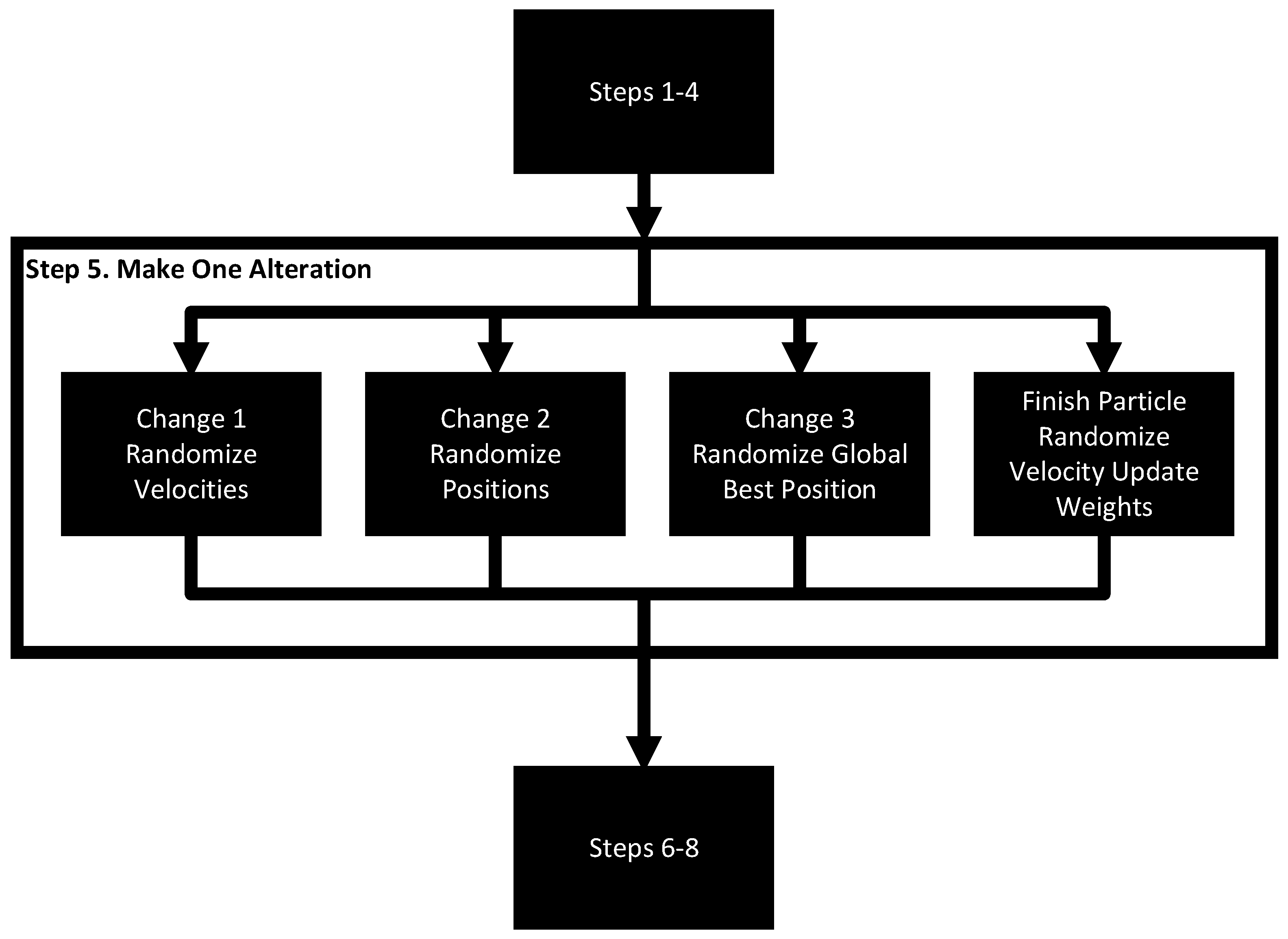
The fifth step, which is depicted in Figure 2, is to alter the copied swarm from step three. The original velocity update formula for particle swarm contained stochastic variables. This would result in a changed final result if the swarm was run beginning at the copied iteration and terminated at the same iteration as the original. One major goal of the proposed technique was for the particles to avoid being trapped by local optima. A concern of using these variables as the only variation from the original swarm and the copied swarm was that they may not provide a great enough change to escape a local optimum in the second particle swarm run. Instead, a deterministic velocity update formula was used, along with other changes, to solve this problem. The determinism of this formula allows for a comparison of the changes presented with fewer stochastic variables altering the results.

In order to test which form of alteration to the copied swarm would be most effective, four different types of changes were analyzed. The first change randomized the velocities of all particles. These velocities were randomized in the same range as they were first randomized. New velocities, at this point, allow each particle to travel to a location very different than they had in the initial particle swarm run. The particles will then travel back toward the global optimum and the particle’s best recorded optimum, allowing for different areas of the search space to be explored. The second change randomized the positions of each particle in the same range as they were first initialized. This also allowed each particle to explore areas of the search space they normally would not explore. It also gives them a head start towards the best global optimum found so far and each particle’s best recorded optimum. The third change randomized the global best position. This change intended to pull particles toward parts of the search space that were not very well explored, while allowing them to also search for better locations along the way. The final change altered the constant values used in the velocity update equation. The inertia weight (w), the individual weight (c₁), and the global weight (c₂) were all changed. These weights began with the values 0.65, 1.15, and 1.15, respectively. The constants were randomized in this change between the ranges of 0.55–0.65, 1.2–1.3, and 1.0–1.1, respectively.

3.6. Step Six: Altered Swarm Run Initiation

The proposed technique continues in the sixth step by initiating a new particle swarm run using the copied and altered particle swarm. This run begins at the same iteration it was copied from in step three. The run will still terminate at the same iteration specified for the first particle swarm run. This means that the second particle swarm run will run for less iterations than the first. For example, if the first run was specified to stop at iteration ten, and was copied at iteration four, the second particle swarm run will go for six iterations. The only alteration to this copied swarm is the change made during the fifth step.

3.7. Step Seven: Swarm Run Completion

Step seven is to finish the particle swarm run. This occurrs automatically when the iteration count reaches the iterations specified by the termination condition. The best position and value of this position is then recorded.

3.8. Step Eight: Swarm Results Comparison

The final step compares the best position recorded by the first and second particle swarm runs. The best position of the two is used as the final output from the technique.

4. Experimental Design

An experiment was performed to test the efficacy of the proposed technique through the comparison of execution times, positions, and optima values. The proposed technique was compared with basic PSO using the velocity update equation presented as Equation (3).

The impact of the four different changes and two different impact calculation methods were compared and tested on four different two-dimensional functions. These functions were chosen because of the high number of local optima, to test the proposed technique’s effectiveness in finding new optima. They also had extremely large domains, and because they are still difficult to optimize even with only two dimensions. Two-dimensional functions were chosen for visualization and easier understanding. The four functions used were:

Function 1:

a(x,y) = −10(((sin(x))/(x)) + ((sin(y))/(y)))

(5)

Function 2:

a(x,y) = ((−10 sin(x))/(x)) + 0.005 y^(2) + 10 sin(y)

(6)

Function 3:

a(x,y) = −((5 sin(x))/(x)) + abs(((x)/(10))) − ((5 sin(y))/(y)) + abs(((y)/(10)))

(7)

Function 4:

a(x,y) = tan^(−1)(x) + sin(x) + 0.1 abs(x) + abs(((y)/(10)))

(8)

The experiment tested each combination of change and impact calculation on each function individually. It was conducted by running the proposed algorithm with each of these differences 1000 times. The algorithm was run with a swarm of ten particles for 100 iterations. The time of the PSO section of the algorithm was recorded to compare with the total time of the algorithm, which was recorded in the same run. The final best position and values of both the regular particle swarm before backtracking to the impactful iteration, and after the entire algorithm had finished were recorded. When all tests were completed, averages of these values were calculated, which are presented in tables in Section 5.

In Section 6, a similar technique was used to collect performance data for several benchmark functions. For these functions, only 100 runs per experimental condition were performed.

5. Data and Analysis

This section presents the results of the experimentation performed using the four functions described in the previous section. Section 5.1 describes and compares the performance and speed of the proposed method with standard PSO. Section 5.2 describes how often and to what extent the proposed technique evicenced improvement over standard particle swarm optimization.

5.1. Performance and Time Comparison

This section compares the different speeds, changes in position, and changes in final value between standard PSO and the proposed technique. The data are organized into multiple tables to compare the efficacy of the technique with regards to different functions, changes, and impact calculations. The column headers for each table in this section are now described in detail.

“PSO Time” refers to the average length of time taken for particle swarm optimization to calculate 100 iterations for ten particles. “Total Time” is the average time taken for the entire proposed technique to run. This includes the time for all steps described in Section 3. The average distance between the final best X1 position of the standard particle swarm run and the run of the proposed technique is represented by “Change in X1.” “Change in X2” is the same as “Change in X1”, but with the X2 positions instead of the X1 positions. “Change in value” is the average change from the PSO algorithm’s final optimum value discovered to the proposed technique’s final optimum value discovered. Lower values for this column mean that the average value improved from the proposed technique. “Value” is the average value of the final optimum value discovered after ten iterations. Negative values are better optima because the test aims to find the global minimum.

The data in this section are divided into three groups to facilitate comparison. These groups show some of the same information from different perspectives.

Table 1. Comparison of function 1.

	PSO Time	Total Time	Change in X1	Change in X2	Change in Value	Value
F1, I1 & C1	1906.74	3656.92	34,078,812	267,861,325	−0.0295	−9.4024
F1, I1 & C2	1837.40	3542.67	26,018,991	283,211,393	0.0034	−9.5030
F1, I1 & C3	2069.83	3952.30	250,289,093	517,481,896	3.0996	−6.2696
F1, I1 & C4	1977.63	3805.72	22,425,846	222,378,901	−0.0513	−9.3670
F1, I2 & C1	2015.62	3986.66	36,024,424	274,591,924	0.1143	−9.2700
F1, I2 & C2	1887.17	3786.91	29,194,097	295,384,920	−0.0172	−9.5209
F1, I2 & C3	1859.88	3697.64	240,798,443	517,338,752	2.9458	−6.4036
F1, I2 & C4	1904.72	3813.94	21,392,322	228,101,911	0.0944	−9.3825

,

Table 2. Comparison of function 2.

	PSO Time	Total Time	Change in X1	Change in X2	Change in Value	Value
F2, I1 & C1	2486.05	4800.38	177,429,539	4.6397	−0.0003	−9.8239
F2, I1 & C2	2469.92	4812.83	206,924,458	4.6868	0.0339	−9.8290
F2, I1 & C3	2434.81	4592.64	633,244,942	420,833,343	48,603,832,417	48,603,832,407
F2, I1 & C4	2421.85	4706.79	93,562,681	5.6614	0.1307	−9.7363
F2, I2 & C1	2437.54	4849.93	188,760,574	4.4250	0.0132	−9.8410
F2, I2 & C2	2441.50	4945.26	209,017,240	5.1077	0.0114	−9.8196
F2, I2 & C3	2418.41	4707.88	642,499,949	433,470,976	85,864,135,795	85,864,135,785
F2, I2 & C4	2417.00	4835.95	92,924,865	5.8958	0.1151	−9.7383

,

Table 3. Comparison of function 3.

	PSO Time	Total Time	Change in X1	Change in X2	Change in Value	Value
F3, I1 & C1	2004.48	3883.06	15.4937	42.0990	2.4393	−4.2073
F3, I1 & C2	1996.79	3877.26	13.7871	13.4733	−0.5233	−7.2252
F3, I1 & C3	2009.03	3824.96	207,643,577	190,931,237	3,155,097	3,155,089
F3, I1 & C4	2037.09	3943.05	34.0384	12.6906	3.7742	−4.0658
F3, I2 & C1	2004.24	4029.31	9.8725	22.3586	−0.3845	−7.0554
F3, I2 & C2	1991.91	4010.13	34.8143	13.8667	2.4043	−4.7250
F3, I2 & C3	1999.80	3943.97	204,505,389	201,069,169	3,354,125	3,354,118
F3, I2& C4	1980.15	3979.76	14.6592	22.7822	1.3499	−5.5003

and

Table 4. Comparison of function 4.

	PSO Time	Total Time	Change in X1	Change in X2	Change in Value	Value
F4, I1 & C1	2141.81	4142.65	12.3266	17.8024	0.3539	−0.1905
F4, I1 & C2	2167.64	4189.43	7.9138	12.0675	−1.0295	−1.3873
F4, I1 & C3	2573.76	4864.35	327,232,859	305,720,882	2,319,123	2,319,122
F4, I1 & C4	2635.89	5110.99	19.9872	14.5960	1.4735	0.6155
F4, I2 & C1	2936.89	5873.21	8.8748	13.7558	0.4099	−0.5241
F4, I2 & C2	2606.76	5216.14	10.9687	13.9923	−1.0635	−1.1463
F4, I2 & C3	2755.83	5404.85	337,688,827	339,171,181	2,352,079	2,352,078
F4, I2 & C4	2717.42	5493.25	78.1190	12.3391	7.8356	6.5991

present the results for functions 1 to 4, respectively. The second group,

Table 5. Comparison of change 1.

	PSO Time	Total Time	Change in X1	Change in X2	Change in Value	Value
F1, I1 & C1	1906.74	3656.92	34,078,812	267,861,325	−0.0295	−9.4024
F2, I1 & C1	2486.05	4800.38	177,429,539	4.6397	−0.0003	−9.8239
F3, I1 & C1	2004.48	3883.06	15.4937	42.0990	2.4393	−4.2073
F4, I1 & C1	2141.81	4142.65	12.3266	17.8024	0.3539	−0.1905
F1, I2 & C1	2015.62	3986.66	36,024,423.56	274,591,924	0.1143	−9.2700
F2, I2 & C1	2437.54	4849.93	188,760,573.76	4.4250	0.0132	−9.8410
F3, I2 & C1	2004.24	4029.31	9.8725	22.3586	−0.3845	−7.0554
F4, I2 & C1	2936.89	5873.21	8.8748	13.7558	0.4099	−0.5241

,

Table 6. Comparison of change 2.

	PSO Time	Total Time	Change in X1	Change in X2	Change in Value	Value
F1, I1 & C2	1837.40	3542.67	26,018,991	283,211,393	0.0034	−9.5030
F2, I1 & C2	2469.92	4812.83	206,924,458	4.6868	0.0339	−9.8290
F3, I1 & C2	1996.79	3877.26	13.7871	13.4733	−0.5233	−7.2252
F4, I1 & C2	2167.64	4189.43	7.9138	12.0675	−1.0295	−1.3873
F1, I2 & C2	1887.17	3786.91	29,194,097	295,384,920	−0.0172	−9.5209
F2, I2 & C2	2441.50	4945.26	209,017,240	5.1077	0.0114	−9.8196
F3, I2 & C2	1991.91	4010.13	34.8143	13.8667	2.4043	−4.7250
F4, I2 & C2	2606.76	5216.14	10.9687	13.9923	−1.0635	−1.1463

,

Table 7. Comparison of change 3.

	PSO Time	Total Time	Change in X1	Change in X2	Change in Value	Value
F1, I1 & C3	2069.83	3952.30	250,289,093	517,481,896	3.0996	−6.2696
F2, I1 & C3	2434.81	4592.64	633,244,942	420,833,343	48,603,832,417	48,603,832,407
F3, I1 & C3	2009.03	3824.96	207,643,577	190,931,237	3,155,097	3,155,089
F4, I1 & C3	2573.76	4864.35	327,232,859	305,720,882	2,319,123	2,319,122
F1, I2 & C3	1859.88	3697.64	240,798,443	517,338,752	2.9458	−6.4036
F2, I2 & C3	2418.41	4707.88	642,499,949	433,470,976	85,864,135,795	85,864,135,785
F3, I2 & C3	1999.80	3943.97	204,505,389	201,069,169	3,354,125	3,354,118
F4, I2 & C3	2755.83	5404.85	337,688,827	339,171,181	2,352,079	2,352,078

and

Table 8. Comparison of change 4.

	PSO Time	Total Time	Change in X1	Change in X2	Change in Value	Value
F1, I1 & C4	1977.63	3805.72	22,425,846	222,378,901	−0.0513	−9.3670
F2, I1 & C4	2421.85	4706.79	93,562,681	5.6614	0.1307	−9.7363
F3, I1 & C4	2037.09	3943.05	34.0384	12.6906	3.7742	−4.0658
F4, I1 & C4	2635.89	5110.99	19.9872	14.5960	1.4735	0.6155
F1, I2 & C4	1904.72	3813.94	21,392,322	228,101,911	0.0944	−9.3825
F2, I2 & C4	2417.00	4835.95	92,924,865	5.8958	0.1151	−9.7383
F3, I2 & C4	1980.15	3979.76	14.6592	22.7822	1.3499	−5.5003
F4, I2 & C4	2717.42	5493.25	78.1190	12.3391	7.8356	6.5991

, is organized by the different changes made in step 5 of the algorithm. Finally,

Table 9. Comparison of impact 1.

	PSO Time	Total Time	Change in X1	Change in X2	Change in Value	Value
F1, I1 & C1	1906.74	3656.92	34,078,812	267,861,325	−0.0295	−9.4024
F1, I1 & C2	1837.40	3542.67	26,018,991	283,211,393	0.0034	−9.5030
F1, I1 & C3	2069.83	3952.30	250,289,093	517,481,896	3.0996	−6.2696
F1, I1 & C4	1977.63	3805.72	22,425,846	222,378,901	−0.0513	−9.3670
F2, I1 & C1	2486.05	4800.38	177,429,539	4.6397	−0.0003	−9.8239
F2, I1 & C2	2469.92	4812.83	206,924,458	4.6868	0.0339	−9.8290
F2, I1 & C3	2434.81	4592.64	633,244,942	420,833,343	48,603,832,417	48,603,832,407
F2, I1 & C4	2421.85	4706.79	93,562,681	5.6614	0.1307	−9.7363
F3, I1 & C1	2004.48	3883.06	15.4937	42.0990	2.4393	−4.2073
F3, I1 & C2	1996.79	3877.26	13.7871	13.4733	−0.5233	−7.2252
F3, I1 & C3	2009.03	3824.96	207,643,577	190,931,237	3,155,097	3,155,089
F3, I1 & C4	2037.09	3943.05	34.0384	12.6906	3.7742	−4.0658
F4, I1 & C1	2141.81	4142.65	12.3266	17.8024	0.3539	−0.1905
F4, I1 & C2	2167.64	4189.43	7.9138	12.0675	−1.0295	−1.3873
F4, I1 & C3	2573.76	4864.35	327,232,859	305,720,882	2,319,123	2,319,122
F4, I1 & C4	2635.89	5110.99	19.9872	14.5960	1.4735	0.6155

and

Table 10. Comparison of impact 2.

	PSO Time	Total Time	Change in X1	Change in X2	Change in Value	Value
F1, I2 & C1	2015.62	3986.66	36,024,424	274,591,924	0.1143	−9.2700
F1, I2 & C2	1887.17	3786.91	29,194,097	295,384,920	−0.0172	−9.5209
F1, I2 & C3	1859.88	3697.64	240,798,443	517,338,752	2.9458	−6.4036
F1, I2 & C4	1904.72	3813.94	21,392,322	228,101,911	0.0944	−9.3825
F2, I2 & C1	2437.54	4849.93	188,760,574	4.4250	0.0132	−9.8410
F2, I2 & C2	2441.50	4945.26	209,017,240	5.1077	0.0114	−9.8196
F2, I2 & C3	2418.41	4707.88	642,499,949	433,470,976	85,864,135,795	85,864,135,785
F2, I2 & C4	2417.00	4835.95	92,924,865	5.8958	0.1151	−9.7383
F3, I2 & C1	2004.24	4029.31	9.8725	22.3586	−0.3845	−7.0554
F3, I2 & C2	1991.91	4010.13	34.8143	13.8667	2.4043	−4.7250
F3, I2 & C3	1999.80	3943.97	204,505,389	201,069,169	3,354,125	3,354,118
F3, I2 & C4	1980.15	3979.76	14.6592	22.7822	1.3499	−5.5003
F4, I2 & C1	2936.89	5873.21	8.8748	13.7558	0.4099	−0.5241
F4, I2 & C2	2606.76	5216.14	10.9687	13.9923	−1.0635	−1.1463
F4, I2 & C3	2755.83	5404.85	337,688,827	339,171,181	2,352,079	2,352,078
F4, I2 & C4	2717.42	5493.25	78.1190	12.3391	7.8356	6.5991

present the two different impact calculation methods.

Some trends can be seen in this data. Function 3 tends to have deviation from the mean values and changes in value more than the other functions, even when change 3 is removed from the calculations. Functions 1, 2, and 4 are more consistent in this regard. Functions 1 and 2 tend to vary much more than functions 3 and 4 for the change in position when not considering change 3. It is likely that these large variations show that the particles in proposed technique ended up in different minima for functions 1 and 2. The time taken for PSO and the proposed technique varies by function.

When comparing the data from the perspective of changes instead of functions, some interesting trends stand out. First, and most notably, change 3 finds consistently worse values, by many orders of magnitude, in all tests. This shows that change 3 does not perform well at finding optimum values. The average time taken for PSO runs is consistent when comparing different changes. This is because the changes do not affect the PSO process. Another notable trend is that the differences between the total time taken for each change vary very little. This demonstrates that the different benefits of the changes have similar costs. Apart from change 3, changes in position are more correlated with the function than with the type of change. This shows that these changes are capable of finding new minima in functions 1 and 2, as was the goal of the technique.

The average of the PSO times for impact calculation 1 was approximately 2198.17. For impact calculation 2, it was approximately 2273.43. The lack of major change here was expected because standard PSO does not use the impact calculation. The average of the total time for iteration 1 was approximately 4231.63, while it was 4535.92 for iteration 2. This is also not a major change. The changes in the other columns, between the two iteration calculation methods, are also minor.

5.2. Improvement Comparison

This section evaluates the frequency of the improvement of the proposed technique and the magnitude of the improvement when it occurs. The table headers for the data presented in this section are now described in detail.

“Runs Improved” represents the percentage of runs, out of 1000, where the proposed technique found a better solution than standard PSO. “Improvement” indicates the average change from the PSO’s final optimum value discovered to the proposed technique’s final optimum value discovered during runs where improvement occurred. This is the same as the “Change in Value” from Section 5.1 with the values where improvement did not occur excluded from the calculation.

The tables in this section are grouped similarly to in Section 5.1. They are split into three groups with each group containing all information from the data in this section. The groups allow for an easier comparison of data.

Table 11. Improvement of function 1.

	Runs Improved	Improvement
F1, I1 & C1	41.7%	−0.8570
F1, I1 & C2	38.7%	−0.8668
F1, I1 & C3	26.1%	−1.5409
F1, I1 & C4	67.3%	−0.5053
F1, I2 & C1	41.7%	−0.8591
F1, I2 & C2	38.0%	−0.8442
F1, I2 & C3	28.4%	−1.4751
F1, I2 & C4	59.5%	−0.4014

,

Table 12. Improvement of function 2.

	Runs Improved	Improvement
F2, I1 & C1	48.3%	−0.2692
F2, I1 & C2	42.4%	−0.2193
F2, I1 & C3	68.0%	−0.1428
F2, I1 & C4	46.1%	−0.1703
F2, I2 & C1	44.3%	−0.2222
F2, I2 & C2	44.8%	−0.2653
F2, I2 & C3	62.0%	−0.0917
F2, I2 & C4	50.8%	−0.1854

,

Table 13. Improvement of function 3.

	Runs Improved	Improvement
F3, I1 & C1	42.9%	−6.1536
F3, I1 & C2	42.1%	−6.1991
F3, I1 & C3	25.7%	−4.2054
F3, I1 & C4	45.2%	−3.2761
F3, I2 & C1	45.3%	−6.0144
F3, I2 & C2	40.1%	−5.3847
F3, I2 & C3	25.9%	−4.0437
F3, I2& C4	43.9%	−5.3050

and

Table 14. Improvement of function 4.

	Runs Improved	Improvement
F4, I1 & C1	45.1%	−2.6140
F4, I1 & C2	48.9%	−2.8208
F4, I1 & C3	15.9%	−3.5479
F4, I1 & C4	47.0%	−1.8359
F4, I2 & C1	44.9%	−1.7645
F4, I2 & C2	49.4%	−3.3121
F4, I2 & C3	17.1%	−0.7406
F4, I2 & C4	42.7%	−1.1226

are grouped by function.

Table 15. Improvement of change 1.

	Runs Improved	Improvement
F1, I1 & C1	41.7%	−0.8570
F2, I1 & C1	48.3%	−0.2692
F3, I1 & C1	42.9%	−6.1536
F4, I1 & C1	45.1%	−2.6140
F1, I2 & C1	41.7%	−0.8591
F2, I2 & C1	44.3%	−0.2222
F3, I2 & C1	45.3%	−6.0144
F4, I2 & C1	44.9%	−1.7645

,

Table 16. Improvement of change 2.

	Runs Improved	Improvement
F1, I1 & C2	38.7%	−0.8668
F2, I1 & C2	42.4%	−0.2193
F3, I1 & C2	42.1%	−6.1991
F4, I1 & C2	48.9%	−2.8208
F1, I2 & C2	38.0%	−0.8442
F2, I2 & C2	44.8%	−0.2653
F3, I2 & C2	40.1%	−5.3847
F4, I2 & C2	49.4%	−3.3121

,

Table 17. Improvement of change 3.

	Runs Improved	Improvement
F1, I1 & C3	26.1%	−1.5409
F2, I1 & C3	68.0%	−0.1428
F3, I1 & C3	25.7%	−4.2054
F4, I1 & C3	15.9%	−3.5479
F1, I2 & C3	28.4%	−1.4751
F2, I2 & C3	62.0%	−0.0917
F3, I2 & C3	25.9%	−4.0437
F4, I2 & C3	17.1%	−0.7406

and

Table 18. Improvement of change 4.

	Runs Improved	Improvement
F1, I1 & C4	67.3%	−0.5053
F2, I1 & C4	46.1%	−0.1703
F3, I1 & C4	45.2%	−3.2761
F4, I1 & C4	47.0%	−1.8359
F1, I2 & C4	59.5%	−0.4014
F2, I2 & C4	50.8%	−0.1854
F3, I2 & C4	43.9%	−5.3050
F4, I2 & C4	42.7%	−1.1226

are grouped by the four changes. The last group is comprised of

Table 19. Improvement of impact 1.

	Runs Improved	Improvement
F1, I1 & C1	41.7%	−0.8570
F1, I1 & C2	38.7%	−0.8668
F1, I1 & C3	26.1%	−1.5409
F1, I1 & C4	67.3%	−0.5053
F2, I1 & C1	48.3%	−0.2692
F2, I1 & C2	42.4%	−0.2193
F2, I1 & C3	68.0%	−0.1428
F2, I1 & C4	46.1%	−0.1703
F3, I1 & C1	42.9%	−6.1536
F3, I1 & C2	42.1%	−6.1991
F3, I1 & C3	25.7%	−4.2054
F3, I1 & C4	45.2%	−3.2761
F4, I1 & C1	45.1%	−2.6140
F4, I1 & C2	48.9%	−2.8208
F4, I1 & C3	15.9%	−3.5479
F4, I1 & C4	47.0%	−1.8359

and

Table 20. Improvement of impact 2.

	Runs Improved	Improvement
F1, I2 & C1	41.7%	−0.8591
F1, I2 & C2	38.0%	−0.8442
F1, I2 & C3	28.4%	−1.4751
F1, I2 & C4	59.5%	−0.4014
F2, I2 & C1	44.3%	−0.2222
F2, I2 & C2	44.8%	−0.2653
F2, I2 & C3	62.0%	−0.0917
F2, I2 & C4	50.8%	−0.1854
F3, I2 & C1	45.3%	−6.0144
F3, I2 & C2	40.1%	−5.3847
F3, I2 & C3	25.9%	−4.0437
F3, I2 & C4	43.9%	−5.3050
F4, I2 & C1	44.9%	−1.7645
F4, I2 & C2	49.4%	−3.3121
F4, I2 & C3	17.1%	−0.7406
F4, I2 & C4	42.7%	−1.1226

, which are organized by the different PSO impact calculations.

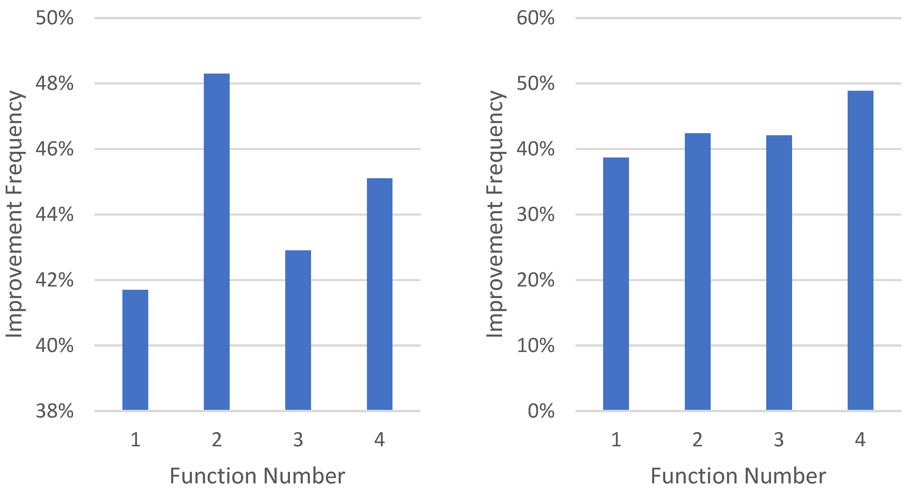
Several conclusions can be drawn from comparing the first group of tables, which compare the different functions. The average values for the column “runs improved” for Table 1, Table 2, Table 3 and Table 4 are 42.7%, 36.2%, 38.9%, and 38.9%, respectively. This shows that the proposed technique was effective most often for function 1, effective less frequently for functions 3 and 4, and effective least often for function 2. The average values for the column “Improvement” for the same tables are −0.92, −0.20, −5.07, and −2.22, respectively. This means that the when the proposed technique improved, it improved much more for function 3 than the other functions. The technique shows the next best improvement for function 4, then function 1, then finally, function 2. Looking at the columns together, the technique performed the worst for function 2 in terms of both metrics.

There are also several notable trends in the data for the second group of tables comparing the efficacy of the changes. First, change 3 improved significantly less often than the other three changes. The average values for the column “runs improved” for change 3 was 19.0%, while for changes 1, 2, and 4, the average values for this column were 44.3%, 43.1%, and 50.3%, respectively. Changes 1 and 2 improved approximately as often as each other. Change 4 improved the most often. The average values for the column “improvement” are −2.34, −2.49, −1.97, and −1.60 for changes 1, 2, 3, and 4, respectively. This data show that change 3 provided the third least improvement when improvement occurred. This, combined with the trend that change 3 improved the least often, shows that the other changes were more effective than change 3. Changes 1 and 2 caused improvement by similar amounts when improvement occurred and improved significantly more than change 4. Change 4 caused improvement by the least on runs where improvement occurred.

When comparing the results for group 3, there is not much difference between the two. The average value for the column “runs improved” is 39.4% for Table 9 and 39.1% for Table 10, while for the column “Improvement” the values are −2.20 for Table 9 and −2.09 for Table 10. This shows that the two different impact calculations are approximately the same in terms of how often they indicate that the proposed technique improved and how much the proposed technique improved. 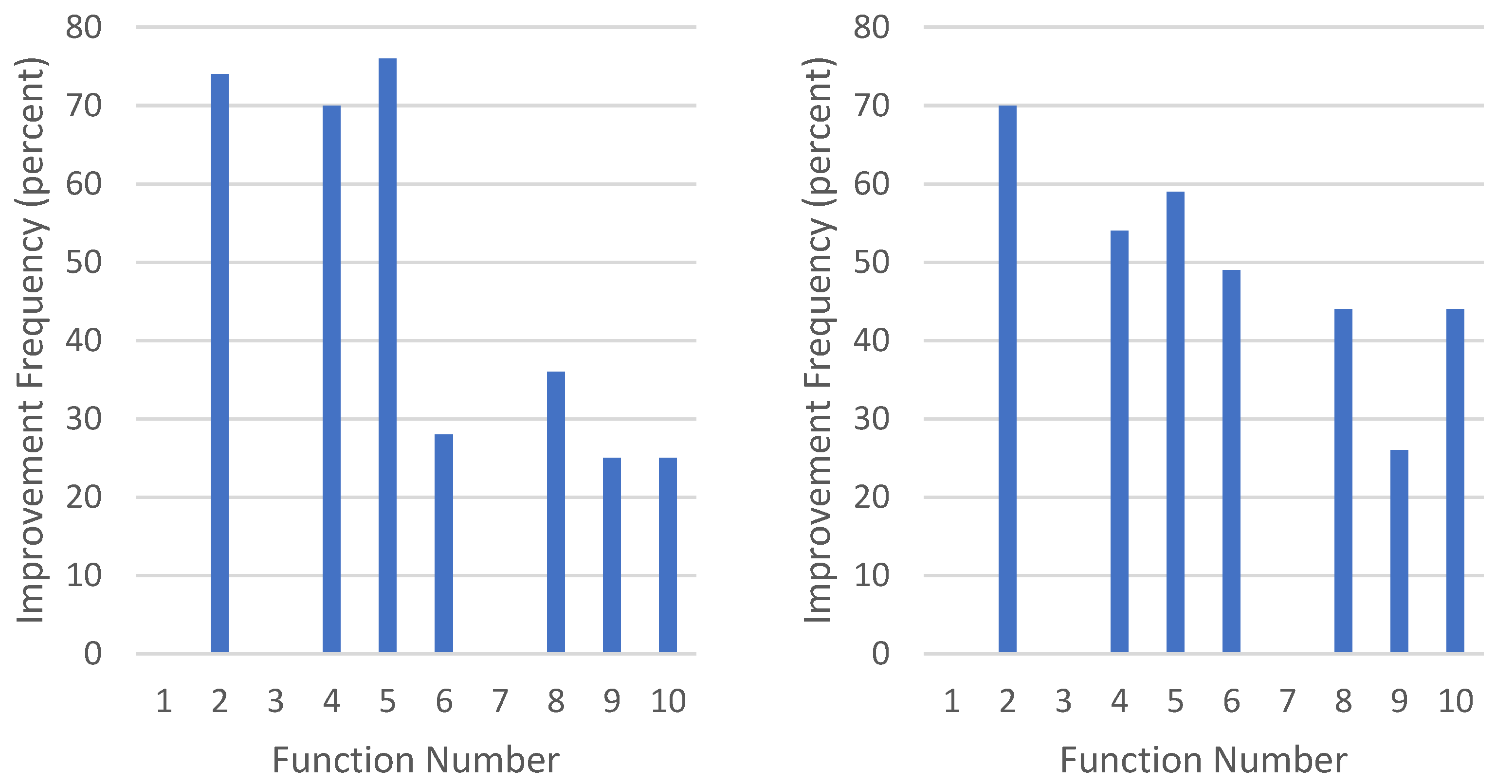Figure 3 and Figure 4 show the frequency of improvement, for each function, for all of the changes.

6. Evaluation with Standard PSO Benchmark Functions

The proposed technique was also tested with ten functions that have been used, in the past, as benchmarks for testing PSO and new techniques based on PSO [76]. This data is presented in

Table 21. Comparison with benchmark function 1.

	PSO Time	Total Time	Change in X	Change in Value	Value	Runs Improved	Improvement
F1, I1 & C1	9318	17,329	0	0	1	0%	N/A
F1, I1 & C2	8940	16,912	0	0	1	0%	N/A
F1, I1 & C3	8925	16,762	0.0247	0	1	0%	N/A
F1, I1 & C4	8846	16,790	0	0	1	0%	N/A
F1, I2 & C1	8971	16,971	0	0	1	0%	N/A
F1, I2 & C2	8968	16,985	0	0	1	0%	N/A
F1, I2 & C3	8957	16,813	−0.1124	0	1	0%	N/A
F1, I2 & C4	8959	16,917	0	0	1	0%	N/A

,

Table 22. Comparison with benchmark function 2.

	PSO Time	Total Time	Change in X	Change in Value	Value	Runs Improved	Improvement
F2, I1 & C1	5064	9580	0.0092	−0.4120	27.2435	50%	−9.6565
F2, I1 & C2	5087	9626	0.0367	7.5621	26.6005	83%	−9.1360
F2, I1 & C3	5173	9720	−0.0005	8.0648	28.5200	74%	−7.9428
F2, I1 & C4	5311	9857	−0.0214	3.8585	26.9951	70%	−5.8806
F2, I2 & C1	5207	9763	0.0552	0.1058	27.7079	52%	−8.9848
F2, I2 & C2	5205	9769	0.0528	7.2876	27.3065	74%	−8.0300
F2, I2 & C3	5167	9738	−0.0549	9.7383	28.7330	80%	−6.4364
F2, I2 & C4	5209	9771	0.0030	1.5293	25.6713	51%	−6.2276

,

Table 23. Comparison with benchmark function 3.

	PSO Time	Total Time	Change in X	Change in Value	Value	Runs Improved	Improvement
F3, I1 & C1	10,283	19,323	0	0	1	0%	N/A
F3, I1 & C2	10,063	19,087	0	0	1	0%	N/A
F3, I1 & C3	10,117	19,119	−13.6258	0	1	0%	N/A
F3, I1 & C4	10,117	19,144	0	0	1	0%	N/A
F3, I2 & C1	10,057	19,080	0	0	1	0%	N/A
F3, I2 & C2	10,147	19,215	0	0	1	0%	N/A
F3, I2 & C3	10,359	19,480	−8.9945	0	1	0%	N/A
F3, I2 & C4	10,191	19,217	0	0	1	0%	N/A

,

Table 24. Comparison with benchmark function 4.

	PSO Time	Total Time	Change in X	Change in Value	Value	Runs Improved	Improvement
F4, I1 & C1	18,297	35,081	0.0216	−391,077	9,682,501	51%	−7,093,880
F4, I1 & C2	18,130	34,914	0.0223	2,934,024	7,950,988	72%	−4,359,232
F4, I1 & C3	18,048	34,785	0.3493	3,345,096	8,617,884	70%	−6,209,680
F4, I1 & C4	18,310	35,131	0.0865	2,065,790	8,335,492	54%	−3,640,395
F4, I2 & C1	18,007	34,736	0.1709	−753,083	7,469,017	48%	−5,543,224
F4, I2 & C2	18,205	34,980	0.0668	2,601,946	7,449,964	72%	−5,552,574
F4, I2 & C3	18,179	34,974	0.0382	3,872,248	9,314,394	70%	−4,400,500
F4, I2 & C4	18,011	34,773	0.1183	1,521,172	9,061,885	62%	−5,372,956

,

Table 25. Comparison with benchmark function 5.

	PSO Time	Total Time	Change in X	Change in Value	Value	Runs Improved	Improvement
F5, I1 & C1	11,606	21,922	−0.0011	0.0493	4.1104	52%	−2.2445
F5, I1 & C2	11,209	21,489	0.0090	1.5136	4.0880	79%	−2.5291
F5, I1 & C3	11,273	21,538	−0.0080	2.0433	4.3406	76%	−1.1821
F5, I1 & C4	11,377	21,645	−0.0024	1.0877	4.6155	59%	−1.3654
F5, I2 & C1	11,263	21,566	0.0006	−0.8312	3.9002	52%	−3.6427
F5, I2 & C2	11,219	21,536	0.0023	1.9756	4.5419	80%	−2.1435
F5, I2 & C3	11,437	21,705	−0.0089	2.7756	5.4746	74%	−2.2397
F5, I2 & C4	11,459	21,754	0.0047	1.4385	5.2161	66%	−1.5336

,

Table 26. Comparison with benchmark function 6.

	PSO Time	Total Time	Change in X	Change in Value	Value	Runs Improved	Improvement
F6, I1 & C1	9629	18,133	5.8234	49.3390	−3068	55%	−749.3261
F6, I1 & C2	9435	17,918	6.3788	11.5119	−3113	53%	−644.3833
F6, I1 & C3	9361	17,676	−20.7022	−584.7923	−3083	28%	−1065.7971
F6, I1 & C4	9359	17,832	−10.6618	3.7847	−2915	49%	−468.4169
F6, I2 & C1	9686	18,351	−1.4783	70.2354	−3048	52%	−577.0189
F6, I2 & C2	9351	17,840	1.5395	81.6112	−3087	56%	−636.2701
F6, I2 & C3	9384	17,758	−33.7632	−368.4185	−3049	31%	−848.1303
F6, I2 & C4	9313	17,826	0.4329	−85.4887	−3037	43%	−608.0977

,

Table 27. Comparison with benchmark function 7.

	PSO Time	Total Time	Change in X	Change in Value	Value	Runs Improved	Improvement
F7, I1 & C1	9657	18,146	0	0	3.7183	0%	N/A
F7, I1 & C2	9485	18,032	0	0	3.7183	0%	N/A
F7, I1 & C3	9389	17,889	0.6205	0	3.7183	0%	N/A
F7, I1 & C4	9459	17,972	0	0	3.7183	0%	N/A
F7, I2 & C1	9687	18,210	0	0	3.7183	0%	N/A
F7, I2 & C2	9756	18,297	0	0	3.7183	0%	N/A
F7, I2 & C3	9451	17,944	−1.5810	0	3.7183	0%	N/A
F7, I2 & C4	9448	17,940	0	0	3.7183	0%	N/A

,

Table 28. Comparison with benchmark function 8.

	PSO Time	Total Time	Change in X	Change in Value	Value	Runs Improved	Improvement
F8, I1 & C1	22,987	44,161	−0.0383	0.1029	−4.6241	52%	−0.8649
F8, I1 & C2	22,849	44,009	−0.0438	0.1850	−4.6897	58%	−0.9351
F8, I1 & C3	22,806	43,804	0.1100	−0.6258	−4.8657	36%	−1.5932
F8, I1 & C4	22,996	44,384	−0.0169	−0.0445	−4.5657	44%	−0.7414
F8, I2 & C1	22,961	44,214	−0.0723	0.1657	−4.6208	54%	−0.8010
F8, I2 & C2	22,859	43,995	−0.0159	0.1207	−4.9178	54%	−0.7732
F8, I2 & C3	22,846	43,935	0.2216	−0.7431	−4.9491	31%	−1.5442
F8, I2 & C4	23,068	44,248	0.0093	−0.0877	−4.8044	41%	−0.8018

,

Table 29. Comparison with benchmark function 9.

	PSO Time	Total Time	Change in X	Change in Value	Value	Runs Improved	Improvement
F9, I1 & C1	5199	9619	0.0466	0.0535	1.0017	24%	−0.5949
F9, I1 & C2	5162	9560	−0.0013	0.0737	0.6616	19%	−0.9214
F9, I1 & C3	5145	9471	0.0304	−0.8746	0.3072	25%	−2.7818
F9, I1 & C4	5102	9516	−0.0666	0.1514	1.1479	26%	0.0000
F9, I2 & C1	5007	9391	−0.0216	−0.1897	1.1415	22%	−1.4582
F9, I2 & C2	5042	9469	−0.0940	0.1708	0.7372	26%	−1.0355
F9, I2 & C3	4971	9270	0.1578	−0.8412	0.7867	27%	−3.6594
F9, I2 & C4	5278	9729	0.0060	0.0155	0.8567	14%	−0.3658

and

Table 30. Comparison with benchmark function 10.

	PSO Time	Total Time	Change in X	Change in Value	Value	Runs Improved	Improvement
F10, I1 & C1	6822	12,704	−0.0494	0.6181	−22.5957	54%	−3.0810
F10, I1 & C2	6734	12,620	−0.1095	0.8752	−21.8569	43%	−2.1479
F10, I1 & C3	6684	12,564	0.0234	−0.7976	−22.9332	25%	−2.8714
F10, I1 & C4	6638	12,614	−0.0540	−0.5018	−22.5002	44%	−4.1088
F10, I2 & C1	6698	12,570	0.0779	0.4714	−22.7737	46%	−2.5588
F10, I2 & C2	6796	12,721	−0.0070	0.5604	−22.8090	45%	−2.5770
F10, I2 & C3	6784	12,688	0.2066	−0.2227	−23.3400	39%	−2.6049
F10, I2 & C4	6799	12,819	0.1804	−0.2463	−23.0105	43%	−3.0330

. Functions 1, 2, 4, 5, and 7 were used to test an improved PSO algorithm in [77]. Functions 1, 2, 3, 4, and 7 were also used for testing another improved PSO algorithm in [78]. Additionally, functions 1, 2, 3, 4, 5, 7, and 10 have been considered when deciding which benchmark functions should be made as an acceptable standard for testing PSO algorithms [79]. All of the functions used for this section were tested with 20 dimensions, except for functions 9 and 10. Functions 1, 3, 6, 8, 9, and 10 are known as the Rastrigin Function, Griewank Function, Schewefel Function, Sine Function, Himmelblau Function, and Shubert Function, respectively [76]. These functions are highly multimodal, which make them effective choices for testing the efficacy of PSO-based techniques. Function 2, the Spherical Function, and function 4 have considerably fewer minima. Function 5 is an interesting function because it adds noise with the random variable to make it more difficult to optimize. These tests were performed in a similar manner as those in Section 5. For each experimental condition, 100 tests of ten particles on 100 iterations were conducted and averaged for each combination of function, impact method, and change.

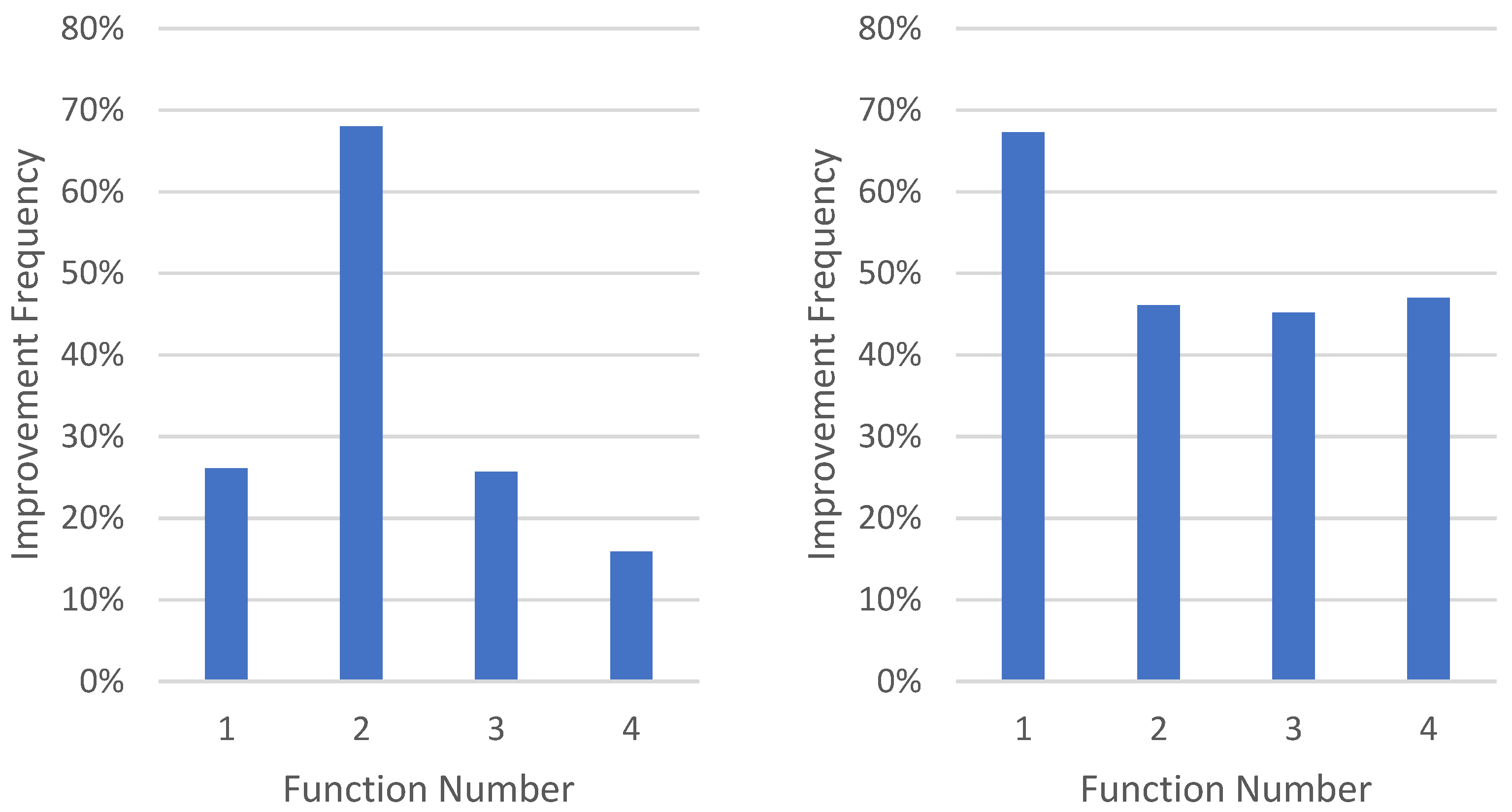
Several conclusions can be drawn from looking at the results of the tests on the benchmark functions. Most notably, change 3 performed much better running against these functions as compared to the functions discussed in Section 5. In Section 5, change 3 was outperformed by the other changes in both improvement frequency and improvement amount on most functions. In this section, change 3 had a significantly higher improvement level for functions 6, 8, and 9 than the other changes. It also improved about as often as the other changes for functions 2 and 9. It also performed well, improving the most or second most often, for functions 4 and 5.

Change 2 performed similarly to these functions as it had for the functions in Section 5. It performed better more often than the other changes, on average, for most functions. This is similar to the results from Section 5. There is a major difference for change 1 with these functions. Change 2 outperformed change 1 notably, in terms of frequency of improvement, for functions 2, 4, and 5. These changes were roughly equal in performance for the tests in Section 5. Change 1 still outperformed change 2 for functions 9 and 10, although not by much.

Similar to change 2, change 4 did about as well for the benchmark functions as it performed in Section 5. Change 4 performed moderately well for the functions in Section 5 and repeated this trend for the benchmark functions. It was rarely the best or the worst change for the benchmark functions in terms of frequency of improvement. In terms of improvement amount, it tended to do worse than all other changes on average. It did show the highest improvement on function 10, however. Figure 5 and Figure 6 show the frequency of improvement, for each function, for all of the changes.

Compared to other algorithms, which have been previously analyzed by others, the approaches proposed herein would appear to outperform some and underperform others. As there are considerable differences in the testing conditions used by prior work, direct comparison has notable limitations. Engelbrecht [78], who noted the importance of the swarm size in comparisons, performed evaluations with a swarm size of ten (as did the work presented herein), among other sizes. Performance with this swarm size ranged from 1.34 to 4.90, with overall values (across all swarm sizes) ranging from 0.00 to 5.08. Pant, Thangaraj, and Abraham [76], using four different algorithms and three different initialization techniques found results as high as 22.34 and as low as nearly 0, for functions with a 0 ideal value. Yi [77], similarly, compared four functions, returning values as high as 52.43 and as low as nearly 0, for functions with a 0 ideal value. This was also the case with the work of Uriarte, Melin, and Valdez [79], who compared two functions and had average values as high as 4.26 and as low as 0 (again, for functions with a 0 ideal value). These prior studies, though, failed to report the percentage or number of runs improved. Additionally, some studies reported far better base PSO results than were seen in this study, further impairing the direct comparison of results. As the techniques proposed herein have the potential to be added to other techniques to further improve their performance, additional study of the discussed techniques and the proposed algorithms’ ability to perform them is a key area of potential future work.

7. Conclusions and Future Work

This paper has proposed a new method for solving optimization problems based upon particle swarm optimization, which has been inspired by science-fiction time travel. It has also presented and analyzed experimentation showing the efficacy of the proposed technique. A description of the proposed technique was provided, experimentation was described in detail, and the effectiveness of the technique was demonstrated using the data presented in Section 5 and Section 6.

The method outlined in this paper, which is based on PSO, uses an eight-step process. It initiates a particle swarm run, calculates the most impactful iteration of the run, copies the swarm at the impactful iteration, terminates the particle swarm run, makes a change to the copied particle swarm, begins a second particle swarm run with the copied particle swarm, terminates the second particle swarm run, compares the results of the two particle-swarm runs, and selects the best solution.

The experimentation described in this paper characterized the efficacy of the proposed technique on four different complex functions and ten standard benchmark functions. The proposed technique was compared to the basic form of PSO. For the proposed technique, four different variations of changes were tested along with two different impact calculation methods.

The analysis of the proposed technique, operating under the four functions presented in Section 5, shows that it is capable of improving PSO’s performance with all four change types. Function 1 experienced improvement the most often, of the functions, and function 3 experienced the most improvement, when improvement occurred. Change 3 produced the worst improvement; however, it might have utility in finding minima, due to the substantial position change it incorporates. Change 4 caused improvement the most often, but caused the least improvement. Changes 1 and 2 caused the most improvement, when improvement occurred, but did not cause improvement as often as change 4 did. Different impact calculation methods were not shown to have a notable effect on the results.

Section 6 showed that all four changes were capable of improving performance for many of the benchmark functions. The changes caused improvement for functions 2, 4, 5, 6, 8, 9, and 10. They did not cause improve for functions 1, 2, and 7. For all three functions, where the technique did not provide an improvement, the technique produced the same results as basic PSO. The results from testing on benchmark functions, in terms of the performance of the different change types, were somewhat different than the four functions presented in Section 5. For the benchmark functions, change three was often more effective than change 4. Change 2 proved to be the most effective change, for the benchmark functions, both in terms of the frequency of improvement and the amount of improvement when change occurred. Change 1 performed second best in regards to both of these metrics. Changes 3 and 4 excelled in different areas from each other. Change 3 performed better in terms of the amount of improvement produced. Change 4 performed better in terms of the frequency of improvement produced.

These findings show that each of the changes could have potential applications. Change 4 could be used in cases where a reliable slight improvement is more important than a lower chance at a high improvement in an optimization problem. Changes 1 and 2 could be used in the opposite situation, where a chance at a high improvement is more important. Change 3 could be used for applications where exploring new areas of a search space is valued the most. The PSO process could potentially be run multiple times or different changes could be used in conjunction with one another to take advantage of their different strengths. For example, the first and second changes could first be used together for a particular application for a larger improvement. If these fail to produce an improvement, change 4 could be used to attempt to achieve a smaller improvement with a higher chance of improvement. Change 3 could also be added in to explore new areas of the search space to find undiscovered minima, while giving a low chance of a high improvement as well. Combinations of the number of iterations and changes might also have some benefit. These, along with trying the technique with other PSO techniques, are all potential areas of future work.

References

1. Karaboga, D.; Basturk, B. On the performance of artificial bee colony (ABC) algorithm. Appl. Soft Comput. J. 2008, 8, 687–697. [Google Scholar] [CrossRef]
2. Yang, X.S.; He, X. Firefly algorithm: Recent advances and applications. Int. J. Swarm Intell. 2013, 1, 36. [Google Scholar] [CrossRef] [Green Version]
3. Dorigo, M.; Blum, C. Ant colony optimization theory: A survey. Theor. Comput. Sci. 2005, 344, 243–278. [Google Scholar] [CrossRef]
4. Yang, X.S.; Deb, S. Cuckoo search: Recent advances and applications. Neural Comput. Appl. 2014, 24, 169–174. [Google Scholar] [CrossRef] [Green Version]
5. Duman, E.; Uysal, M.; Alkaya, A.F. Migrating Birds Optimization: A new metaheuristic approach and its performance on quadratic assignment problem. Inf. Sci. 2012, 217, 65–77. [Google Scholar] [CrossRef]
6. Clerc, M. Particle Swarm Optimization; Wiley: Hoboken, NY, USA, 2010; pp. 1942–1948. [Google Scholar] [CrossRef]
7. Poli, R. Analysis of the Publications on the Applications of Particle Swarm Optimisation. J. Artif. Evol. Appl. 2008, 2008, 685175. [Google Scholar] [CrossRef]
8. Zhang, Y.; Wang, S.; Ji, G. A Comprehensive Survey on Particle Swarm Optimization Algorithm and Its Applications. Math. Probl. Eng. 2015, 2015, 931256. [Google Scholar] [CrossRef] [Green Version]
9. Liu, Y.; Qin, Z.; Shi, Z.; Lu, J. Center particle swarm optimization. Neurocomputing 2007, 70, 672–679. [Google Scholar] [CrossRef]
10. Liu, B.; Wang, L.; Jin, Y.H.; Tang, F.; Huang, D.X. Improved particle swarm optimization combined with chaos. Chaos Solitons Fractals 2005, 25, 1261–1271. [Google Scholar] [CrossRef]
11. Kao, Y.T.; Zahara, E. A hybrid genetic algorithm and particle swarm optimization for multimodal functions. Appl. Soft Comput. J. 2008, 8, 849–857. [Google Scholar] [CrossRef]
12. Laporte, G. A concise guide to the Traveling Salesman Problem. J. Oper. Res. Soc. 2010, 61, 35–40. [Google Scholar] [CrossRef]
13. Brucal, S.G.E.; Dadios, E.P. Comparative analysis of solving traveling salesman problem using artificial intelligence algorithms. In Proceedings of the 2017 IEEE 9th International Conference on Humanoid, Nanotechnology, Information Technology, Communication and Control, Environment and Management (HNICEM), Manila, Philippines, 1–3 December 2017; pp. 1–6. [Google Scholar] [CrossRef]
14. Ayache, N. Medical computer vision, virtual reality and robotics. Image Vis. Comput. 1995, 13, 295–313. [Google Scholar] [CrossRef] [Green Version]
15. Rowley, H.A.; Member, S.; Baluja, S.; Kanade, T. Neural Network-Based Face Detection. IEEE Trans. Pattern Anal. Mach. Intell. 1998, 20, 23–38. [Google Scholar] [CrossRef]
16. Liang, M.; Hu, X. Recurrent convolutional neural network for object recognition. In Proceedings of the 2015 IEEE Conference on Computer Vision and Pattern Recognition (CVPR), Boston, MA, USA, 7–12 June 2015; pp. 3367–3375. [Google Scholar] [CrossRef]
17. Indurkhya, B. Multi-Agent Blackboard Architecture. Comput. Sci. 2018, 19, 457–477. [Google Scholar]
18. Liao, S.H. Expert system methodologies and applications-a decade review from 1995 to 2004. Expert Syst. Appl. 2005, 28, 93–103. [Google Scholar] [CrossRef]
19. Straub, J.; Reza, H. The use of the blackboard architecture for a decision making system for the control of craft with various actuator and movement capabilities. In Proceedings of the ITNG 2014 11th International Conference on Information Technology: New Generations, Las Vegas, NV, USA, 7–9 April 2014. [Google Scholar]
20. Cheng, M.Y.; Lien, L.C. A hybrid AI-based particle bee algorithm for facility layout optimization. Eng. Comput. 2012, 28, 57–69. [Google Scholar] [CrossRef]
21. Amisha; Malik, P.; Pathania, M.; Rathuar, V.K. Overview of artificial intelligence in medicine. J. Fam. Med. Prim. Care 2019, 8, 2328. [Google Scholar] [CrossRef]
22. Abduljabbar, R.; Dia, H.; Liyanage, S.; Bagloee, S.A. Applications of artificial intelligence in transport: An overview. Sustainability 2019, 11, 189. [Google Scholar] [CrossRef] [Green Version]
23. Surden, H. Artificial intelligence and law: An Overview. Ga. State Univ. Law Rev. 2019, 35, 1306–1337. [Google Scholar]
24. Chassignol, M.; Khoroshavin, A.; Klimova, A.; Bilyatdinova, A. Artificial Intelligence trends in education: A narrative overview. Procedia Comput. Sci. 2018, 136, 16–24. [Google Scholar] [CrossRef]
25. Graham, S.; Depp, C.; Lee, E.E.; Nebeker, C.; Tu, X.; Kim, H.C.; Jeste, D.V. Artificial Intelligence for Mental Health and Mental Illnesses: An Overview. Curr. Psychiatry Rep. 2019, 21, 116. [Google Scholar] [CrossRef] [PubMed]
26. Lu, W.; Tong, Y.; Yu, Y.; Xing, Y.; Chen, C.; Shen, Y. Applications of Artificial Intelligence in Ophthalmology: General Overview. J. Ophthalmol. 2018, 2018, 5278196. [Google Scholar] [CrossRef] [PubMed] [Green Version]
27. Martínez-López, F.J.; Casillas, J. Artificial intelligence-based systems applied in industrial marketing: An historical overview, current and future insights. Ind. Mark. Manag. 2013, 42, 489–495. [Google Scholar] [CrossRef]
28. Parpinelli, R.S.; Lopes, H.S. New inspirations in swarm intelligence: A survey. Int. J. Bio-Inspired Comput. 2011, 3, 1–16. [Google Scholar] [CrossRef]
29. Dorigo, M.; Stützle, T. Ant Colony Optimization: Overview and Recent Advances. In Handbook of Metaheuristics; Springer: New York, NY, USA, 2019; Volume 272, pp. 311–351. [Google Scholar]
30. Forestiero, A.; Mastroianni, C.; Spezzano, G. Antares: An ant-inspired P2P information system for a self-structured grid. In Proceedings of the 2007 2nd Bio-Inspired Models of Network, Information and Computing Systems, Budapest, Hungary, 10–12 December 2007; pp. 151–158. [Google Scholar] [CrossRef]
31. Karaboga, D.; Basturk, B. A powerful and efficient algorithm for numerical function optimization: Artificial bee colony (ABC) algorithm. J. Glob. Optim. 2007, 39, 459–471. [Google Scholar] [CrossRef]
32. Bansal, J.C.; Sharma, H.; Jadon, S.S.; Clerc, M. Spider Monkey Optimization algorithm for numerical optimization. Memetic Comput. 2014, 6, 31–47. [Google Scholar] [CrossRef]
33. Abdel-Basset, M.; Abdel-Fatah, L.; Sangaiah, A.K. Metaheuristic Algorithms: A Comprehensive Review. Comput. Intell. Multimed. Big Data Cloud Eng. Appl. 2018, 185–231. [Google Scholar] [CrossRef]
34. Forestiero, A. Metaheuristic algorithm for anomaly detection in Internet of Things leveraging on a neural-driven multiagent system. Knowl.-Based Syst. 2021, 228, 107241. [Google Scholar] [CrossRef]
35. Poli, R.; Kennedy, J.; Blackwell, T. Particle swarm optimization: An overview. Swarm Intell. 2007, 1, 33–57. [Google Scholar] [CrossRef]
36. Eberhart, R.C.; Shi, Y. Particle swarm optimization: Developments, applications and resources. In Proceedings of the 2001 Congress on Evolutionary Computation, Seoul, Korea, 27–30 May 2001; Volume 1, pp. 81–86. [Google Scholar] [CrossRef]
37. Mohaghegi, S.; Del Valle, Y.; Venayagamoorthy, G.K.; Harley, R.G. A comparison of PSO and backpropagation for training RBF neural networks for identification of a power system with statcom. In Proceedings of the 2005 IEEE Swarm Intelligence Symposium (2005 SIS), Pasadena, CA, USA, 8–10 June 2005; pp. 391–394. [Google Scholar] [CrossRef]
38. Che, Z.H. PSO-based back-propagation artificial neural network for product and mold cost estimation of plastic injection molding. Comput. Ind. Eng. 2010, 58, 625–637. [Google Scholar] [CrossRef]
39. AlRashidi, M.R.; El-Hawary, M.E. A survey of particle swarm optimization applications in electric power systems. IEEE Trans. Evol. Comput. 2009, 13, 913–918. [Google Scholar] [CrossRef]
40. Doctor, S.; Venayagamoorthy, G.K.; Gudise, V.G. Optimal PSO for collective robotic search applications. In Proceedings of the 2004 Congress on Evolutionary Computation, Portland, OR, USA, 19–23 June 2004; Volume 2, pp. 1390–1395. [Google Scholar] [CrossRef]
41. Chiam, S.C.; Tan, K.C.; Mamun, A. Al A memetic model of evolutionary PSO for computational finance applications. Expert Syst. Appl. 2009, 36, 3695–3711. [Google Scholar] [CrossRef]
42. Hajihassani, M.; Jahed Armaghani, D.; Kalatehjari, R. Applications of Particle Swarm Optimization in Geotechnical Engineering: A Comprehensive Review. Geotech. Geol. Eng. 2018, 36, 705–722. [Google Scholar] [CrossRef]
43. Grimaldi, E.A.; Grimaccia, F.; Mussetta, M.; Zich, R.E. PSO as an effective learning algorithm for neural network applications. In Proceedings of the 2004 3rd International Conference on Computational Electromagnetics and Its Applications (ICCEA 2004), Beijing, China, 1–4 November 2004; pp. 557–560. [Google Scholar] [CrossRef]
44. Liu, B.; Li, J.; Lin, W.; Bai, W.; Li, P.; Gao, Q. K-PSO: An improved PSO-based container scheduling algorithm for big data applications. Int. J. Netw. Manag. 2021, 31, e2092. [Google Scholar] [CrossRef]
45. Masehian, E. Particle Swarm Optimization Methods, Taxonomy and Applications. Int. J. Comput. Theory Eng. 2009, 1, 486. [Google Scholar]
46. Kashyap, A.K.; Parhi, D.R. Particle Swarm Optimization aided PID gait controller design for a humanoid robot. ISA Trans. 2021, 114, 306–330. [Google Scholar] [CrossRef] [PubMed]
47. Fan, Y.; Wang, P.; Heidari, A.A.; Chen, H.; Turabieh, H.; Mafarja, M. Random reselection particle swarm optimization for optimal design of solar photovoltaic modules. Energy 2022, 239, 121865. [Google Scholar] [CrossRef]
48. Ceylan, Z. Short-term prediction of COVID-19 spread using grey rolling model optimized by particle swarm optimization. Appl. Soft Comput. 2021, 109, 107592. [Google Scholar] [CrossRef]
49. Kan, X.; Fan, Y.; Fang, Z.; Cao, L.; Xiong, N.N.; Yang, D.; Li, X. A novel IoT network intrusion detection approach based on Adaptive Particle Swarm Optimization Convolutional Neural Network. Inf. Sci. 2021, 568, 147–162. [Google Scholar] [CrossRef]
50. Zaman, H.R.R.; Gharehchopogh, F.S. An improved particle swarm optimization with backtracking search optimization algorithm for solving continuous optimization problems. Eng. Comput. 2021, 1, 1–35. [Google Scholar] [CrossRef]
51. Li, N.; Wang, J.; Wu, L.; Bentley, Y. Predicting monthly natural gas production in China using a novel grey seasonal model with particle swarm optimization. Energy 2021, 215, 119118. [Google Scholar] [CrossRef]
52. Houssein, E.H.; Gad, A.G.; Hussain, K.; Suganthan, P.N. Major Advances in Particle Swarm Optimization: Theory, Analysis, and Application. Swarm Evol. Comput. 2021, 63, 100868. [Google Scholar] [CrossRef]
53. Han, F.; Chen, W.T.; Ling, Q.H.; Han, H. Multi-objective particle swarm optimization with adaptive strategies for feature selection. Swarm Evol. Comput. 2021, 62, 100847. [Google Scholar] [CrossRef]
54. Gu, Q.; Wang, Q.; Li, X.; Li, X. A surrogate-assisted multi-objective particle swarm optimization of expensive constrained combinatorial optimization problems. Knowl.-Based Syst. 2021, 223, 107049. [Google Scholar] [CrossRef]
55. Ji, X.; Zhang, Y.; Gong, D.; Sun, X. Dual-Surrogate-Assisted Cooperative Particle Swarm Optimization for Expensive Multimodal Problems. IEEE Trans. Evol. Comput. 2021, 25, 794–808. [Google Scholar] [CrossRef]
56. Li, A.D.; Xue, B.; Zhang, M. Improved binary particle swarm optimization for feature selection with new initialization and search space reduction strategies. Appl. Soft Comput. 2021, 106, 107302. [Google Scholar] [CrossRef]
57. Sedighizadeh, D.; Masehian, E.; Sedighizadeh, M.; Akbaripour, H. GEPSO: A new generalized particle swarm optimization algorithm. Math. Comput. Simul. 2021, 179, 194–212. [Google Scholar] [CrossRef]
58. Liu, X.; Zhang, D.; Zhang, J.; Zhang, T.; Zhu, H. A path planning method based on the particle swarm optimization trained fuzzy neural network algorithm. Cluster Comput. 2021, 24, 1901–1915. [Google Scholar] [CrossRef]
59. Song, X.F.; Zhang, Y.; Gong, D.W.; Gao, X.Z. A Fast Hybrid Feature Selection Based on Correlation-Guided Clustering and Particle Swarm Optimization for High-Dimensional Data. IEEE Trans. Cybern. 2021, 1–14. [Google Scholar] [CrossRef]
60. Wang, F.; Zhang, H.; Zhou, A. A particle swarm optimization algorithm for mixed-variable optimization problems. Swarm Evol. Comput. 2021, 60, 100808. [Google Scholar] [CrossRef]
61. Song, X.; Zhang, Y.; Gong, D.; Sun, X. yan Feature selection using bare-bones particle swarm optimization with mutual information. Pattern Recognit. 2021, 112, 107804. [Google Scholar] [CrossRef]
62. Islam, M.R.; Ali, S.M.; Fathollahi-Fard, A.M.; Kabir, G. A novel particle swarm optimization-based grey model for the prediction of warehouse performance. J. Comput. Des. Eng. 2021, 8, 705–727. [Google Scholar] [CrossRef]
63. Kashani, A.R.; Chiong, R.; Mirjalili, S.; Gandomi, A.H. Particle Swarm Optimization Variants for Solving Geotechnical Problems: Review and Comparative Analysis. Arch. Comput. Methods Eng. 2021, 28, 1871–1927. [Google Scholar] [CrossRef]
64. Thakkar, A.; Chaudhari, K. A Comprehensive Survey on Portfolio Optimization, Stock Price and Trend Prediction Using Particle Swarm Optimization. Arch. Comput. Methods Eng. 2021, 28, 2133–2164. [Google Scholar] [CrossRef]
65. Pervaiz, S.; Ul-Qayyum, Z.; Bangyal, W.H.; Gao, L.; Ahmad, J. A Systematic Literature Review on Particle Swarm Optimization Techniques for Medical Diseases Detection. Comput. Math. Methods Med. 2021, 2021, 5990999. [Google Scholar] [CrossRef]
66. Baccolini, R. The Persistence of Hope in Dystopian Science Fiction raffaella baccolini. PMLa 2004, 119, 518–521. [Google Scholar]
67. Westfahl, G. Space and Beyond: The Frontier Theme in Science Fiction; Greenwood Press: Westport, CT, USA, 2000. [Google Scholar]
68. Bell, F.; Fletcher, G.; Greenhill, A.; Griffiths, M.; McLean, R. Science fiction prototypes: Visionary technology narratives between futures. Futures 2013, 50, 15–24. [Google Scholar] [CrossRef]
69. Potstada, M.; Zybura, J. The role of context in science fiction prototyping: The digital industrial revolution. Technol. Forecast. Soc. Chang. 2014, 84, 101–114. [Google Scholar] [CrossRef]
70. Lobo, F.S.N. Closed timelike curves and causality violation. Class. Quantum Gravity Theory Anal. Appl. 2012, 6, 283–310. [Google Scholar]
71. Wells, H. Time Machine. In The Time Traveler’s Almanac; Ann, V., Jeff, V., Eds.; William Heinemann: London, UK, 1895; pp. 154–157. [Google Scholar]
72. Asimov, I. What If. In The Time Traveler’s Almanac; Ann, V., Jeff, V., Eds.; Fantastic Story Magazine: Kokomo, IN, USA, 1952; pp. 678–687. [Google Scholar]
73. Rooden, T.; Eg, P.; Valkenburg, R.; Transfer, K.; Innovation, P. Time Travel, a Method for Playful Future-Oriented User Research. Nordes 2011, 1–5. Available online: https://dl.designresearchsociety.org/cgi/viewcontent.cgi?article=1262&context=nordes (accessed on 16 February 2022).
74. Shi, Y. Particle Swarm Optimization. IEEE Neural Netw. Soc. 2004, 2, 8–13. [Google Scholar]
75. McCaffrey, J. Artificial Intelligence—Particle Swarm Optimization. MSDN Magazine. August 2011. Available online: https://docs.microsoft.com/en-us/archive/msdn-magazine/2011/august/artificial-intelligence-particle-swarm-optimization (accessed on 13 April 2022).
76. Pant, M.; Thangaraj, R.; Abraham, A. Particle Swarm Optimization: Performance Tuning and Empirical Analysis. Stud. Comput. Intell. 2009, 203, 101–128. [Google Scholar] [CrossRef] [Green Version]
77. Yi, L. Study on an Improved PSO Algorithm and its Application for Solving Function Problem. Int. J. Smart Home 2016, 10, 51–62. [Google Scholar] [CrossRef]
78. Engelbrecht, A.P. Fitness function evaluations: A fair stopping condition? In Proceedings of the 2014 IEEE Symposium on Swarm Intelligence, Orlando, FL, USA, 9–12 December 2014; pp. 181–188. [Google Scholar] [CrossRef]
79. Uriarte, A.; Melin, P.; Valdez, F. An improved Particle Swarm Optimization algorithm applied to Benchmark Functions. In Proceedings of the 2016 IEEE 8th International Conference on Intelligent Systems (IS), Sofia, Bulgaria, 4–6 September 2016; pp. 128–132. [Google Scholar] [CrossRef]
Figure 1. Eight-step process of the proposed technique.
Ai 03 00024 g001
Figure 2. Algorithm change options.
Ai 03 00024 g002
Figure 3. Improvement frequencies for changes 1 (left) and 2 (right).
Ai 03 00024 g003
Figure 4. Improvement frequencies for changes 3 (left) and 4 (right).
Ai 03 00024 g004
Figure 5. Improvement frequencies for changes 1 (left) and 2 (right).
Ai 03 00024 g005
Figure 6. Improvement frequencies for changes 3 (left) and 4 (right).
Ai 03 00024 g006