Performance Evaluation of Deep Neural Network Model for Coherent X-ray Imaging

Abstract

We present a supervised deep neural network model for phase retrieval of coherent X-ray imaging and evaluate the performance. A supervised deep-learning-based approach requires a large amount of pre-training datasets. In most proposed models, the various experimental uncertainties are not considered when the input dataset, corresponding to the diffraction image in reciprocal space, is generated. We explore the performance of the deep neural network model, which is trained with an ideal quality of dataset, when it faces real-like corrupted diffraction images. We focus on three aspects of data qualities such as a detection dynamic range, a degree of coherence and noise level. The investigation shows that the deep neural network model is robust to a limited dynamic range and partially coherent X-ray illumination in comparison to the traditional phase retrieval, although it is more sensitive to the noise than the iteration-based method. This study suggests a baseline capability of the supervised deep neural network model for coherent X-ray imaging in preparation for the deployment to the laboratory where diffraction images are acquired.

1. Introduction

Phase retrieval problems, meaning the problem of recovering a complex-valued object from intensities alone, are a ubiquitous challenge spanning from quantum physics, electron microscopy, crystallography, X-ray imaging and astronomy [1,2,3,4,5]. In coherent X-ray diffractive imaging (CDI), the X-ray beam illuminates an object of interest and diffracted intensities are measured in the far field. It is essential to solve the phase retrieval problem in CDI to reconstruct the image of an object in real space. The phase retrieval employing an iterative method provides a unique solution when the particular requirements for the convergence are satisfied [6,7]. In experiments, an object has to be illuminated by a coherent X-ray beam and the data should be well oversampled [8,9]. In the image reconstruction process, at least several hundreds of iterations are needed and multiple runs with a random guess of initial phases are required to gain a reliable solution [10,11,12]. The fundamental idea for the iteration-based approach is that the function goes back and forth between real and reciprocal space by using Fourier transformation repeatedly. During the iterations, it is refined by the constraints until it reaches a converged solution in real space [13,14,15,16]. Coherent X-ray diffractive imaging has grown to be a powerful technique to explore in situ and operando dynamics of materials at the modern X-ray sources such as synchrotron storages and fourth-generation X-ray free-electron lasers [17,18,19,20,21,22]. Despite the advantages, it does not deliver a solution in a timely manner due to the iterative nature.

It has been demonstrated that a deep neural network-based method, which is a non-iterative end-to-end method, provides rapid results for phase retrieval in 2D and 3D coherent X-ray imaging [23,24,25,26]. Moreover, there have been rapid progresses for optical tomography [27,28], ghost imaging [29,30], face detection [31], growth stage detection [32], and low photon imaging [33]. In addition, an unsupervised approach has been developed to overcome the limitations that the supervised neural networks can have due to aiming for matching a particular label [34,35]. In the future, a deep learning-based image reconstruction is expected to be deployed and used in a laboratory where diffraction images are collected. Most proposed supervised neural network models have a tacit assumption that diffraction images for the training and test are collected under flawless and ideal experimental conditions. For instance, the models assume that input image data has a constant degree of dynamic range, noise-free, and fully coherent illumination. There are, however, inherently technical limitations in experiments, preventing us from obtaining an accurate and clear diffraction image [36,37]. In reality, there are various experimental uncertainties including an imperfection of optical elements, vacuum quality in the beam transport system, and detector performance, etc. The combinations of these parameters affect the resultant quality of diffraction images. The conventional phase retrieval algorithm has been continuously improved to be robust to the low quality of actual images obtained from experiments [38,39,40,41,42]. Since the ultimate goal of neural network models for the phase retrieval is to perform the best with the actual diffraction images, it is crucial to understand how sensitive the model is to different aspects of image qualities and find a baseline capability of the model. We present a supervised deep neural network model for image prediction based on the diffraction images and conducted the evaluation of the performance in a systematic way.

2. Materials and Methods

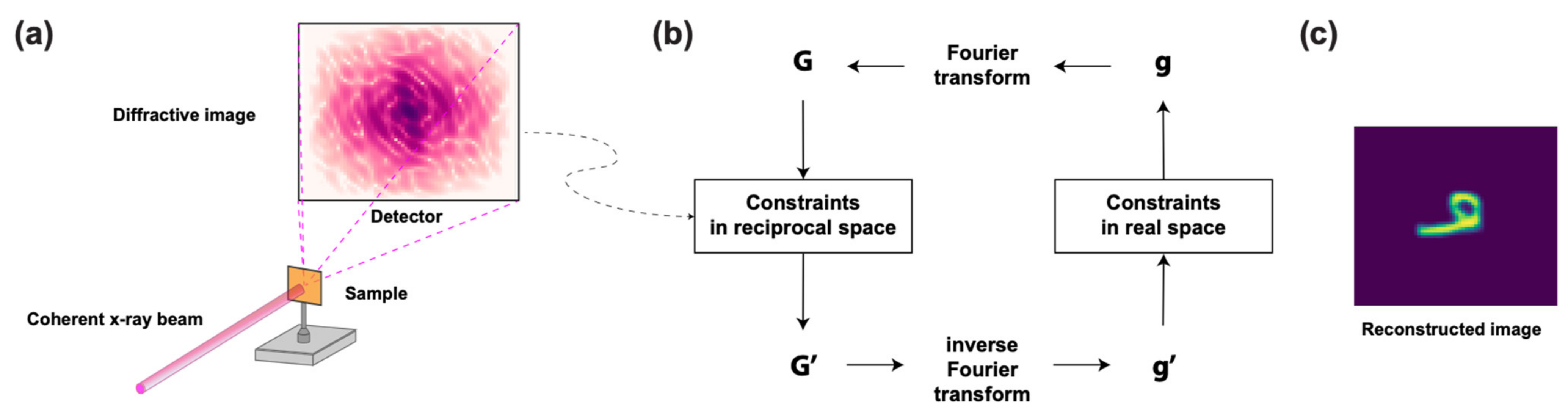
2.1. Coherent X-ray Imaging

We consider the diffraction phenomenon in the kinetic regime, which can be analytically described using the classical formulation of the kinetic scattering of X-rays from crystalline materials [43] as shown in Figure 1a. It allows the Fourier transformation relationship between an object and its measured intensity [38].

$$f\left(x\right)=\left|f\left(x\right)\right|exp\left[i\eta \left(x\right)\right]$$

(1)

where $f\left(x\right)$ is a complex-valued object and $\eta \left(x\right)$ is its phase. The Fourier transformation of the object is expressed as follows [38].

$$F\left(u\right)=\left|F\left(u\right)\right|exp\left[i\psi \left(u\right)\right]=FT\left[f\left(x\right)\right]$$

(2)

where FT denotes the Fourier Transformation. The goal of phase retrieval is to find an amplitude and phase of $f\left(x\right)$ with a given $\left|F\left(u\right)\right|$, which is from the intensity recorded on a detector. In order to recover a complex-valued object, the Gerchberg–Saxton (G-S) algorithm [38], which is the iteration-based phase retrieval algorithm, is widely used. While a complex-valued function is going back and forth between real and reciprocal space, the constraints are applied in each space and eventually a converged solution is obtained, which is an object image that consists of amplitude and phase. The concept of the G-S algorithm and an example of converged solution are displayed in Figure 1b and Figure 1c, respectively. The real space constraints ensure that the amplitude outside of the support, in which the object is assumed to exist is set to zero. In reciprocal space, the amplitude of complex-value is replaced with the square root of intensity.

The Gerchberg–Saxton (G-S) algorithm [38] consists of iterating over the following four steps. (1) Fourier transform an estimate of the object; (2) replace the modulus of the resulting computed Fourier transform with measured Fourier modulus; (3) inverse Fourier transform the updated function in (2); and (4) replace the modulus of the computed inverse transform with the measured object modulus as the estimated object in a new round of iteration. It can be written in expressions as follows:

$$G_k\left(u\right)=\left|G_k\left(u\right)\right|exp\left[i{\varnothing }_k\left(u\right)\right]=FT\left[g_k\left(x\right)\right]$$

(3)

$$G{\prime }_k\left(u\right)=\left|F\left(u\right)\right|exp\left[i{\varnothing }_k\left(u\right)\right]$$

(4)

$$g{\prime }_k\left(x\right)=\left|g{\prime }_k\left(x\right)\right|exp\left[i\theta {\prime }_k\left(x\right)\right]=F{T}^{-1}\left[G{\prime }_k\left(u\right)\right]$$

(5)

$$g_{k+1}\left(x\right)=\left|f\left(x\right)\right|exp\left[i{\theta }_{k+1}\left(x\right)\right]=\left|f\left(x\right)\right|exp\left[i\theta {\prime }_k\left(x\right)\right]$$

(6)

where $g_k$, ${\theta }_k$, $G{\prime }_k$, and ${\varnothing }_k$ are estimates of f, η, F and ψ, respectively. In the case of error-reduction (ER) algorithm [38], the first three steps are identical to that of G-S algorithm, and fourth step is given by

$$g_{k+1}\left(x\right)=\left\{\begin{array}{c}g{\prime }_k\left(x\right), if x\in \gamma \\ 0, if x\notin \gamma \end{array}\right.$$

(7)

where $\gamma$ is the set of points where real space constraints are not violated. The hybrid input-output (HIO) algorithm [38] is modified from ER algorithm.

$$g_{k+1}\left(x\right)=\left\{\begin{array}{c}g{\prime }_k\left(x\right), if x\in \gamma \\ g_k\left(x\right)-\beta g{\prime }_k\left(x\right), if x\notin \gamma \end{array}\right.$$

(8)

where β is a constant ranging from 0 to 1. Unlike the G-S algorithm, our approach is to train an end-to-end deep neural network model so that we can obtain a solution instantly without the refinement. The process flows as follows: First, we develop a deep convolutional neural network model for phase retrieval of coherent X-ray imaging. This is the model trained and tested with the ideal diffraction images generated based on the X-ray scattering theory. Once it is confirmed that the model is reliable, the diffraction images with artifacts are fed into it.

2.2. Scope of Image Qualities

Among many different kinds of artifacts in diffraction images, we focus on those associated with a spatial resolution and occur inevitably in experiments such as a detection dynamic range, a degree of coherence and noise level. The diffraction images that have artifacts are manipulated from ideal images by adding noises or blurring with convolution of Gaussian filters or cutting intensities below certain thresholds. Depending on the artifacts on diffraction images, the performance of the deep neural network model would be poorer than in the absence of artifacts. Similarly, the iterative phase retrieval algorithm can produce reconstructed images that contain artifacts or fail to converge at all.

2.2.1. Degree of Coherence

Needless to say, the illuminating wavefields are required to be coherent in coherent X-ray imaging. However, most coherent X-ray imaging experiments are performed at third-generation synchrotron or electron sources that are not fully coherent, although highly coherent [44,45,46]. In practice, the majority of the synchrotron undulator sources have a limited degree of partial coherence, leading to a lower speckle contrast in coherent diffraction images [47]. If it is assumed that the incoming X-ray is fully coherent, there is a simple Fourier transformation relationship between the object shape and its diffracted intensity. However, the recorded intensity from partially coherent illumination is as follows [36,43,48].

$$I_{pc}\left(q\right)=I_c\left(q\right)\otimes \widehat{\gamma }\left(q\right)$$

(9)

where $I_{pc}\left(q\right)$ and $I_c\left(q\right)$ are the partially coherent intensity and fully coherent intensity, respectively. $\widehat{\gamma }\left(q\right)$ is the Fourier transformation of mutual coherence function (MCF) and $\otimes$ denotes a convolutional operator.

The effect of Equation (9) is blurring the coherent intensity by convolution with the Fourier transform of the normalized MCF [49], which is assumed to be a 2D Gaussian distribution.

2.2.2. Detection Dynamic Range

A dynamic range is an extent of modulation in diffraction images and the diffracted intensity decays dramatically with a spatial frequency. Because a dynamic range contributes to a spatial resolution in coherent X-ray imaging, it is crucial to increase the dynamic range as much as possible while avoiding the damage of samples by the adjustment of exposure time or accumulation of repeated exposures [50,51]. The detection dynamic range is limited by the susceptibility of a sample to the X-ray beam, and the capability of a detector including the robustness to an electrical uncertainty and the efficiency of a detection. In this study, we apply different thresholds for the minimum intensity by enforcing the intensity below it zero to generate various dynamic ranges in diffraction images [52].

2.2.3. Noise Level

A noise is one of the artifacts that contributes to the degradation of diffraction images. Any deviation of the measured intensity from the true intensity can make errors in the reconstruction of images [53]. Sources of noise can include shot noise, any X-ray signal from external sources and the noise associated with thermal and mechanical uncertainty of experimental setup [40]. In X-ray diffraction experiments, there is an inherent uncertainty in the measurement of arriving photons governed by the Poisson distribution, commonly known as shot noise. It is widely used in the CDI community for testing algorithms [54]. The intrinsic signal-to-noise ratio due to the photon counting shot noise can be improved by increasing exposure.

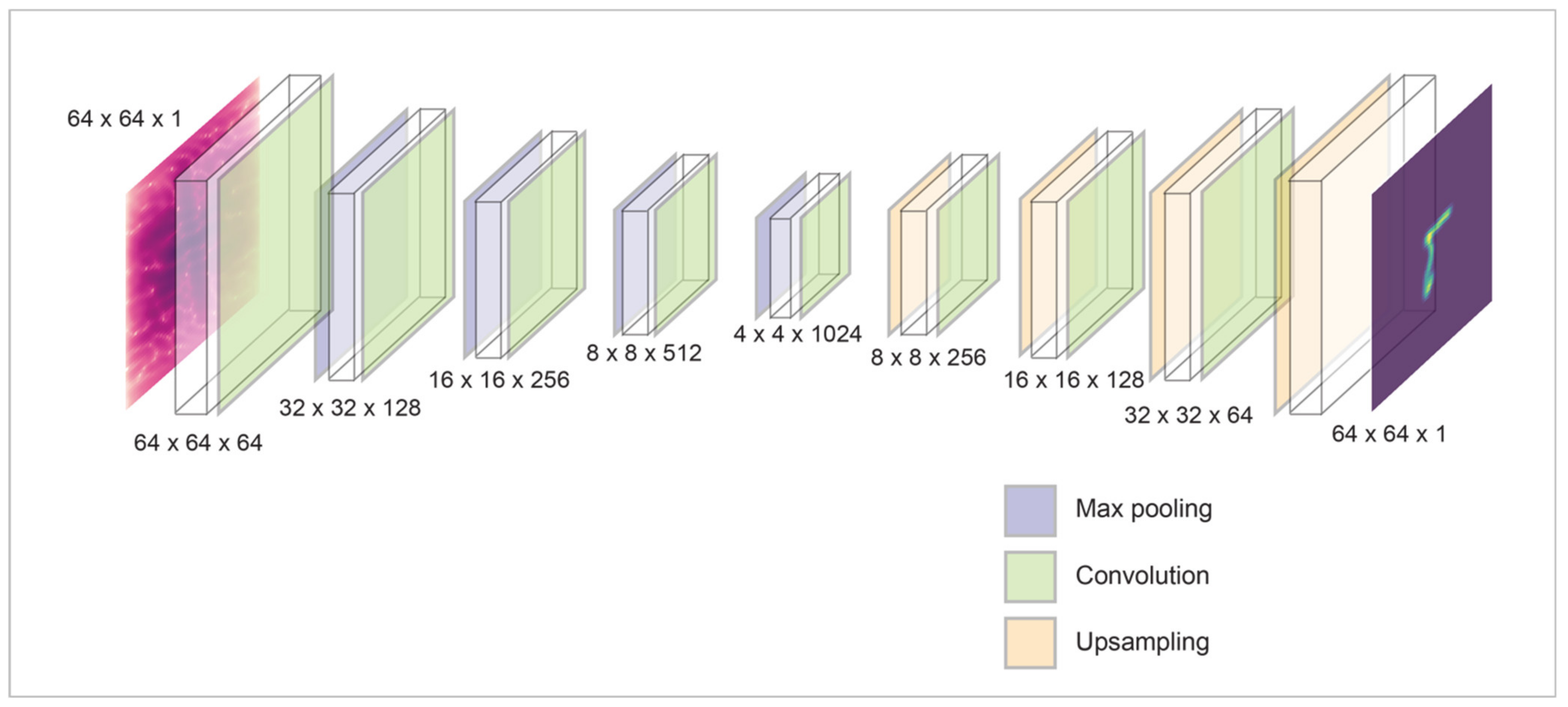
2.3. Architecture and Parameters of Convolutional Neural Network

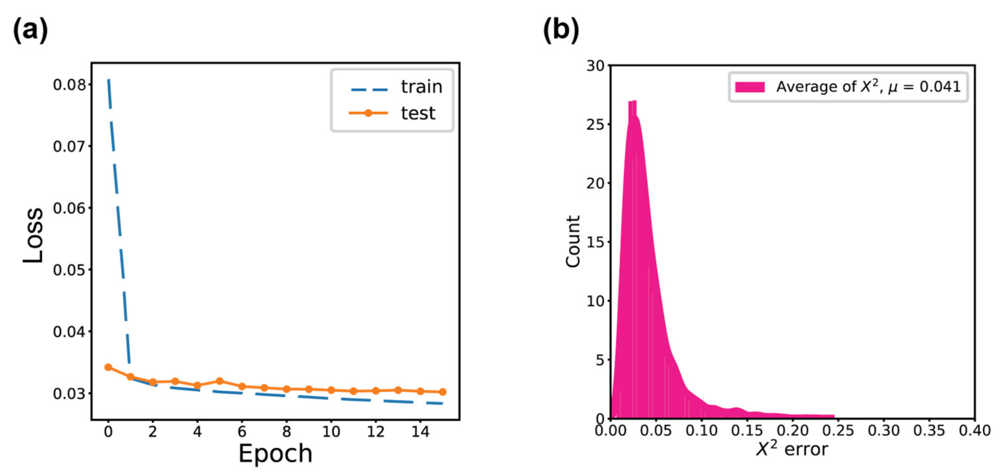
As presented in Figure 2, the deep neural network for coherent X-ray diffraction imaging employs an encoder-decoder architecture. It takes an intensity of 2D coherent X-ray diffraction pattern in reciprocal space as input and real-space amplitude images are considered as outputs. The architecture is based on the studies of convolutional deep learning neural networks for coherent X-ray imaging [23,24,25,26,55,56,57]. The proposed model is implemented using an architecture composed entirely of 2D convolutional, max-pooling, and upsampling layers. In this 2D deep convolutional neural network, the rectified linear unit (ReLU) is used for all activation functions except for the last 2D convolutional layer, where the sigmoid activation function is used. The convolutional neural network has two convolutional layers of filter size of 3 × 3 and the max-sampling layer with a pool size of 2 × 2. A max-sampling layer follows each convolutional layer. The convolutional and pooling layers together extract the features of the image. The parameters of the network, as well as the kernel, are updated during the training process until the desired accuracy is achieved. Figure 3a shows the training and validation loss as a function of epochs. Each epoch refers to one complete pass of the training data. We trained the networks for 16 epochs using a batch size of 32. At each step, we used adaptive moment estimation (ADAMS) [58] with a learning rate of 0.001 to update the weights, while the loss (or error metric) for both training and validation was computed using cross-entropy. It also shows that the training and validation loss decrease and are saturated finally as the epoch increases. Since no divergence occurs in the validation loss, it is indicative of the stability of our model. In addition, the $X^2$ error, which is widely used to evaluate the quality of reconstruction images in phase retrieval methods, is employed in this study.

$$X^2=\frac{{{\displaystyle \sum }}_{i=1}^{N_p}{\left(\sqrt{I_p^i}-\sqrt{I_g^i}\right)}^2}{{{\displaystyle \sum }}_{i=1}^{N_p}{I}_g^i}$$

(10)

where $I_p^i$ and $I_g^i$ are the reconstructed X-ray diffraction intensity, and the ground-truth diffraction intensity in the i-th pixel, respectively. $N_p$ denotes the number of pixels in an image. The average (μ) of $X^2$ error over 6000 test images is 0.041 for our deep neural network model as shown in Figure 3b.

Training was performed on the NVIDIA Tesla K80 GPU using the Keras package running the Tensorflow backend [59]. The training for each network took about 15 min for 16 epochs. We employ a publicly available dataset, which is a handwritten Kannada language, termed Kannada-MNIST [60]. These handwritten images and corresponding diffraction images were used for the output and input data, respectively. The dataset consists of 54,000 pairs of gray-scale images for training, and a test set of 6000 sample images uniformly distributed across the 10 classes. We enlarged 28 × 28-pixel-size of original images to 64 × 64-pixel-size images by padding zero matrices that allowed us to not only train a deep learning model, but also conduct a traditional phase retrieval because the zero padding around the sample image results in the oversampling on diffraction images [8]. The ideal diffraction images were used for pre-training and the degraded images were used for the evaluation of the model.

3. Results

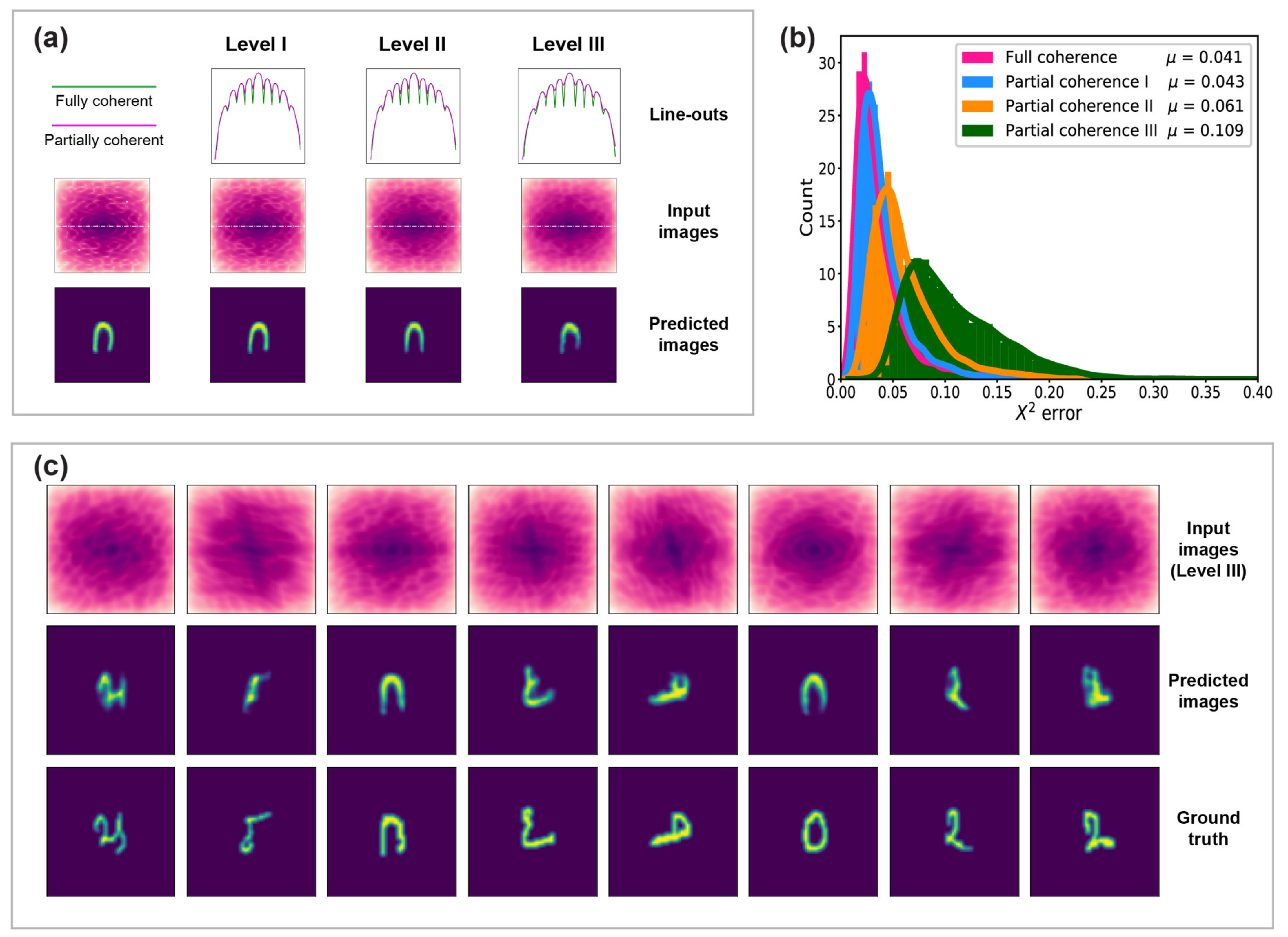
3.1. Degree of Coherence

In Figure 4a, there are four input and output images, corresponding to the diffraction images and object images that result from the deep neural network model, respectively. The left side image of the second row is a fully coherent diffraction image, and the rest three images are partially coherent diffraction images. Three different degrees of partial coherence are made with different standard deviations of Gaussian filters such as 0.42, 0.55 and 0.78 pixel, which are defined as the level I, II and III, respectively. The first row shows 1-D plots of the horizontal lines depicted as white dashed lines on the images of the second row. Needless to say, as the X-ray beam is less coherent, the diffraction image is more blurred. The level III diffraction images are significantly smoothed out, so that the iterative phase retrieval method fails to converge or ends up having greater than 0.5 of the $X^2$ error. The $X^2$ errors are averaged over 6000 test datasets for each level. As the degree of coherence deviates from a full coherence, the $X^2$ error shifts to the right moderately as shown in Figure 4b. There has been progress in improving the phase retrieval algorithms to mitigate the effect of partial coherence [36,47]. However, the advanced algorithm to mitigate the partially coherent illumination is not included in the iterative phase retrieval process since the partial coherence is not taken into account when the neural network model is trained. However, despite the lack of coherence, it is observed that there are reasonable matches between true object images and the predictions based on the level III of diffraction images as shown in Figure 4c.

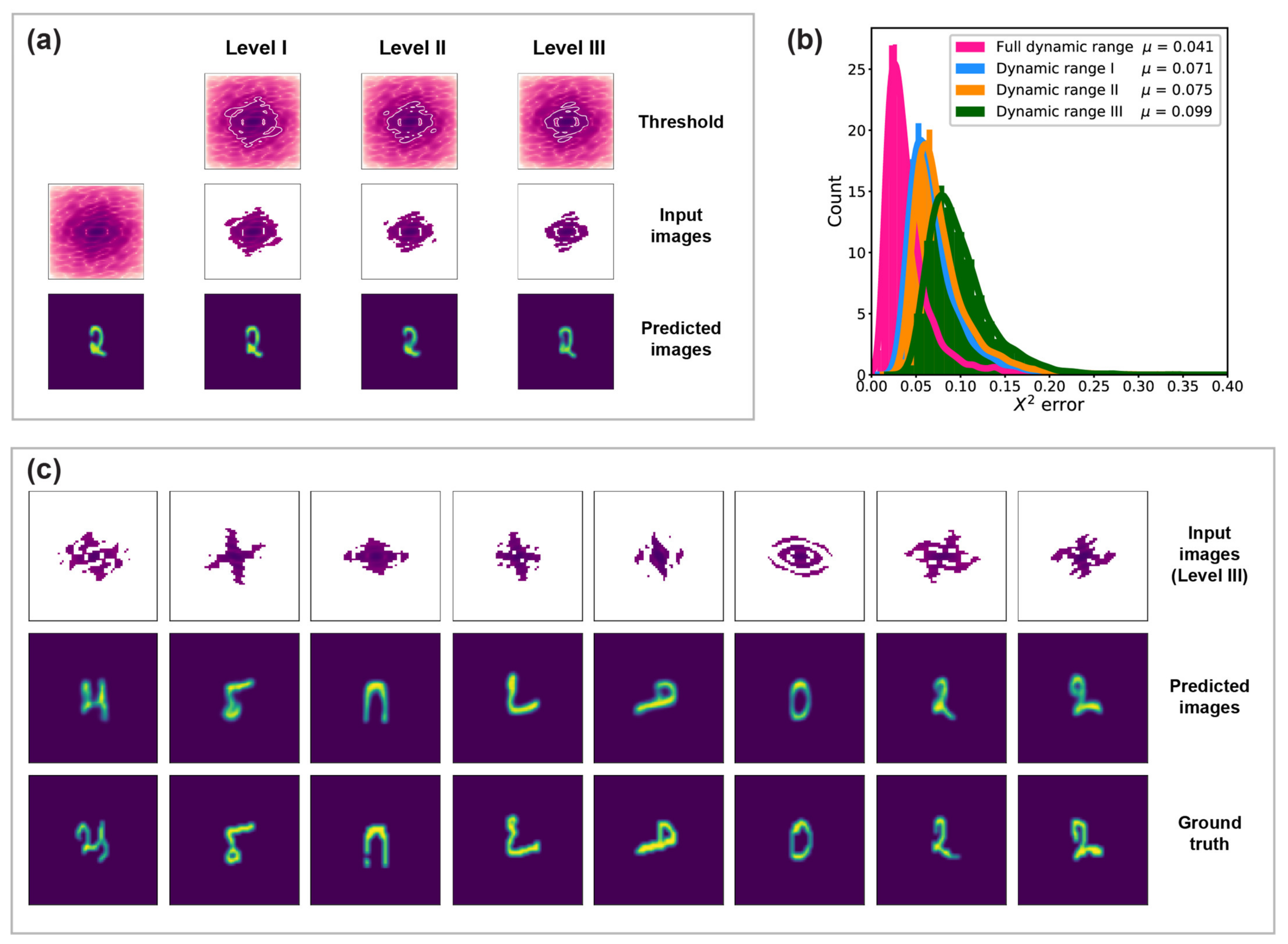
3.2. Detection Dynamic Range

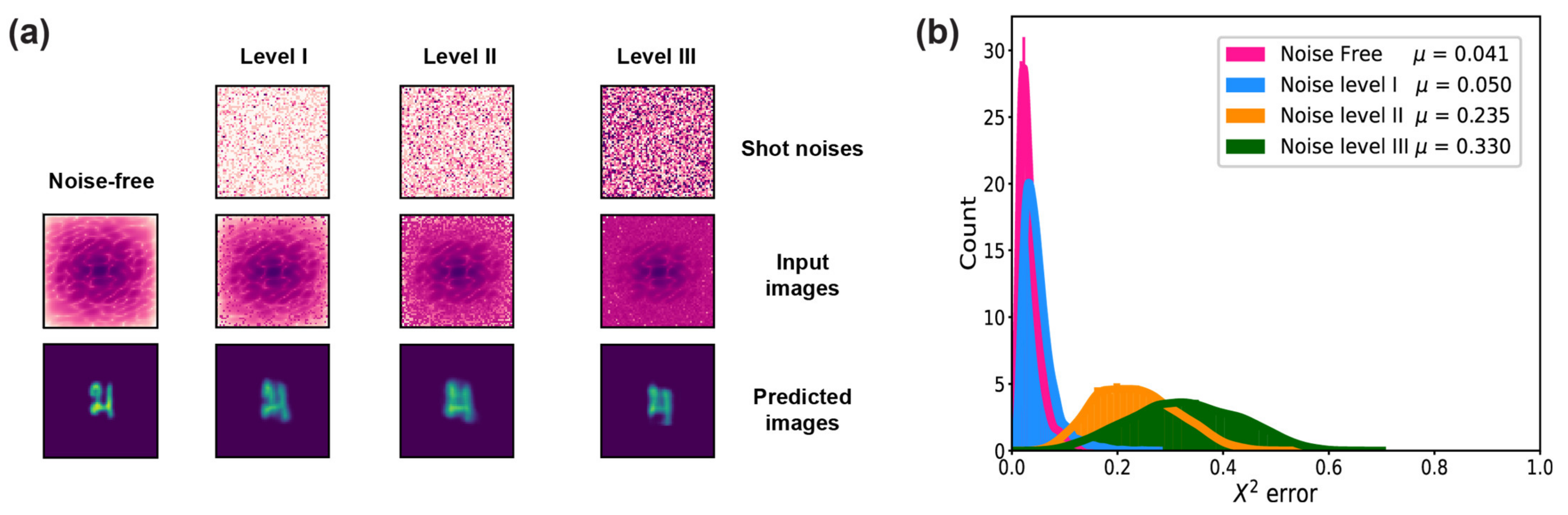
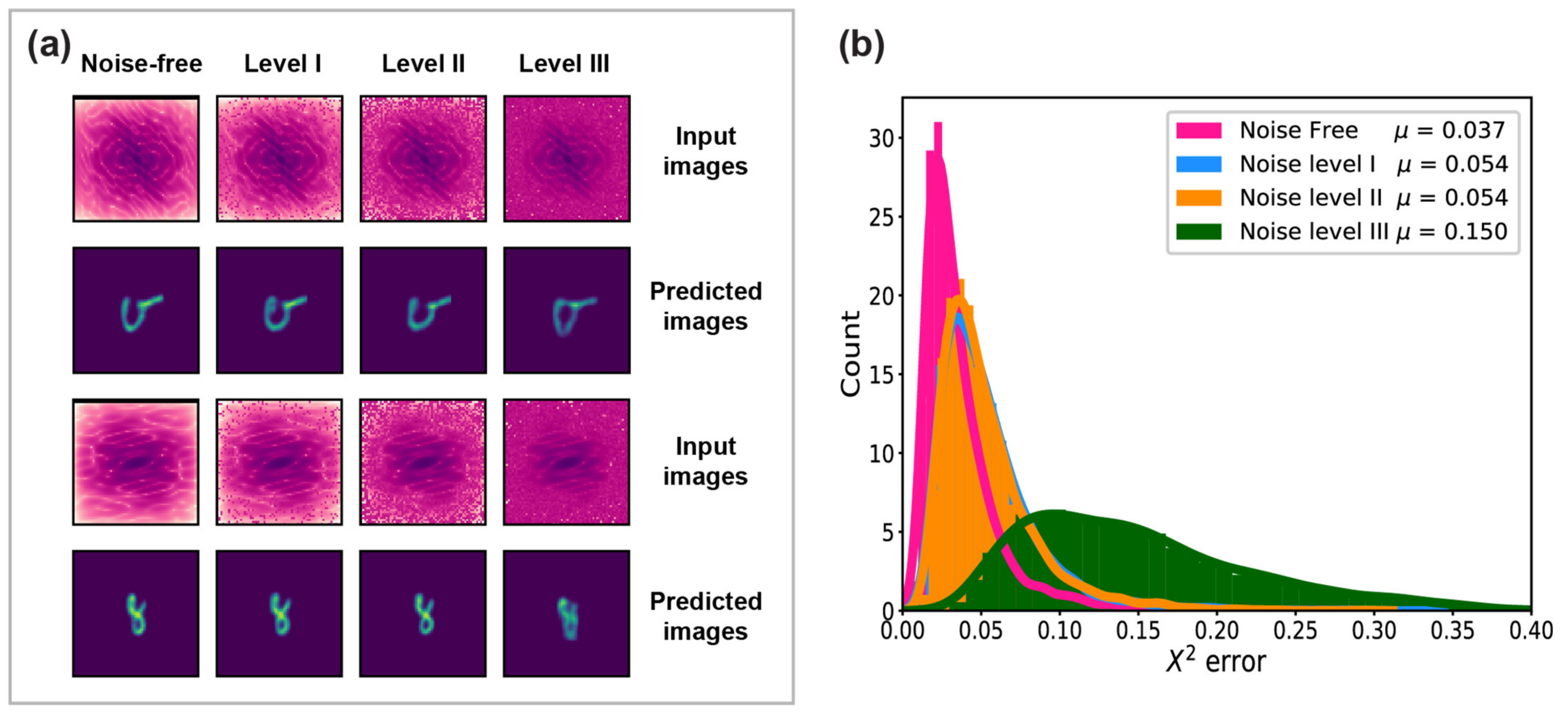
Figure 5a shows four input diffraction images and corresponding object images predicted by the neural network model. The input image on the left side of the second row has the same detection dynamic range as the pre-training dataset and the rest three images have shorter dynamic ranges. The images in the first row include white contours below which the intensities are removed as shown in the second row. The thresholds chosen to limit the dynamic range are 0.4%, 0.6%, and 0.8% of the maximum intensity, which are named as the level I, II, and III of dynamic ranges, respectively. Figure 5b shows that as the dynamic range becomes shorter, the average of $X^2$ error increases. The effective number of pixels is calculated circularly. It is an average extent from a center to the farthest pixel above the threshold and they are 29.1, 26.8 and 25.0 out of 32 for the level I, II, and III, respectively. It is revealed that the dynamic range of the level III is too short to enable the iterative phase retrieval method to produce a converged solution. However, the deep neural network model shows excellent performance in predicting the object image from the same level of dynamic range as shown in Figure 5c. It implies that the model is capable of predicting an object image while data are acquired, for example, repeated exposure of sample to X-ray beam to accumulate diffraction images.

3.3. Noise Level

Shot noises following a Poisson distribution are added to the artifact-free diffraction images. Figure 6a shows four input images and corresponding predicted images from the neural network model. The input images are noise-free and three different levels of noisy diffraction images. We introduced Poisson-distributed noise and calculated the signal-to-noise ratio (SNR) as the ratio of the power of the diffracted intensity to the power of the noise [61]. The SNRs are 10⁶, 10⁵, and 10⁴ for level I, II, and III, respectively. The average (μ) of $X^2$ error drastically increases when the SNRs are 10⁵ or less than that as shown in Figure 6b. With the level III noises, the traditional phase retrieval provides solutions that have lower $X^2$ error than the neural network model.

4. Discussion

4.1. Degree of Coherence

To quantify a degree of coherence with respect to an object, we use a ratio of the standard deviation of mutual coherence function (MCF) to the size of the object. The standard deviation of mutual coherence function (MCF), which is related to the degree of coherence [36], can be calculated based on the formula $\mathsf{\sigma }=\mathrm{N}/\left(2\mathsf{\pi }\widehat{\sigma }\right)$ with $\mathrm{N}$ the number of pixels across the image, which is 64 and the standard deviations of the Gaussian filter in reciprocal space $\widehat{\sigma }$, which are 0.42, 0.55 and 0.78 pixel. These result in 24.3, 18.5, and 13.1 of the standard deviations of MCF for the level I, II, and III, respectively. Since the average size of objects is 18.5 × 18.5 pixels in 64 × 64-pixel images, the ratios of the standard deviations of MCF to the size of objects are 1.3, 1.0, and 0.7 for the level I, II, and III, respectively. It indicates that the model robustly handles the various degrees of coherence when the mutual coherence function is 30% larger, equal to or 30% smaller than the object size. The performances depending on a relative size of MCF are found in

Table 1. Performance of the neural network model depends on the degree of coherence, which is defined as the ratio of the size of the mutual coherence function (i.e., standard deviation) to the size of the object.

Relative Size of MCF	1.3	1.0	0.7
$X^2$	0.043	0.061	0.109

.

4.2. Detection Dynamic Range

The detection dynamic range can be measured by the number of meaningful pixels from a center to the farthest point. In this regard, the detection dynamic range is defined by the ratio of the effective number of pixels to the total number of pixels across a half size of image. Thus, the level I, II, and III has 91%, 84%, and 78% of detection dynamic ranges, respectively. The average $X^2$ errors depending on a detection dynamic range are shown in

Table 2. Performance of the neural network model depends on the detection dynamic range, which is defined as the ratio of the number of meaningful pixels from a center to the total number of pixels across a half size of image.

Detection Dynamic Range	91%	84%	78%
$X^2$	0.071	0.075	0.099

.

4.3. Noise Level

As a coherent X-ray image deviates from ideal quality, it is obvious that the performances of both iterative feedback-based algorithms and end-to-end algorithms become worse. In the former case, a diffractive image leads a convergence of solution to an inaccurate direction and in the latter case, the prediction is less reliable due to the lack of similarity between the images used in pre-training and actual input image. Therefore, the approach to enhance the accuracy of iterative models is to improve the quality of diffractive images such as denoising images [62] or to improve noise tolerance in phase retrieval process [63,64], whereas the effort to increase the reliability of end-to-end model is to make the images for pre-training similar to the input images fed into the model [56].

The test images are generated with SNRs ranging from 10⁶ to 10⁴ to mimic noise levels that are typical of Bragg coherent diffractive imaging measurements at synchrotron facilities (10⁴) up to those anticipated at XFEL light sources (10⁶) [61]. Our approach is to predict object images with coherent X-ray images based on the non-iterative end-to-end algorithm. If a noise is unavoidable and its level is known, it would be more effective to train the model with noisy images than with noise-free images for the non-iterative end-to-end methods.

A new model is trained with the level II noisy diffraction images, which has the SNR 10⁵. Figure 7a shows noise-free input images, three different levels of input images, and corresponding predicted images. Figure 7b shows that the performance is improved considerably, and the model performs better with noise-free images than the level II noisy images, which are used for pre-training. Unlike the dynamic range and the degree of coherence, the noise level is sensitive to the performance of the neural network model, compared to the traditional phase retrieval method. However, if the model is trained with noisy diffraction images, the noise robustness is improved significantly. A summary of the performance is shown in

Table 3. Performance of the neural network model trained with noisy diffraction images, which has the SNR 10⁵.

Signal-to-Noise Ratio	106	105	104
$X^2$	0.054	0.054	0.150

.

5. Conclusions

In summary, we present a supervised deep neural network model for coherent X-ray imaging and characterize the performance. The ideal diffraction patterns are simulated based on the kinetic scattering theory and additional datasets are generated by the degradation of the original dataset to mimic realistic experimental diffraction images. The artifact-free images are used to train the deep neural network model and corrupted diffraction images are fed into the model to predict the object images. To the best of our knowledge, the artifacts in the neural networks for coherent X-ray imaging have not been addressed adequately. The systemic analysis shows that the model provides reliable solutions despite the low quality of detection dynamic range and partially coherent illumination. However, the noisy diffraction images cause poor performance in comparison to the traditional iterative phase retrieval. An efficient strategy to mitigate the negative effects of noises is to incorporate the noise to the pre-training dataset. As the conventional phase retrieval has been improved enormously over the past decade while facing the low quality of experimental data, the deep learning model for phase retrieval in coherent X-ray imaging is expected to be advanced continuously from the baseline capability that is suggested in this study.

References

1. Paul, H. Phase retrieval in quantum mechanics. Phys. Rev. A 1994, 50, R921–R924. [Google Scholar]
2. Zuo, J.M.; Vartanyants, I.; Gao, M.; Zhang, R.; Nagahara, L.A. Atomic Resolution Imaging of a Carbon Nanotube from diffraction intensities. Science 2003, 300, 1419–1422. [Google Scholar] [CrossRef] [PubMed] [Green Version]
3. Miao, J.; Charalambous, R.; Kirz, J.; Sayre, D. Extending the methodology of x-ray crystallography to allow imaging of micrometre-sized non-crystalline specimens. Nature 1999, 400, 342–344. [Google Scholar] [CrossRef]
4. Gerchberg, R.W.; Saxton, W.O. A practical algorithm for the determination of phase from image and diffraction plane pictures. Optik 1972, 35, 237–246. [Google Scholar]
5. Dainty, J.C.; Fienup, J.R. Phase retrieval and image reconstruction for astronomy. In Image Recovery: Theory and Application; Stark, H., Ed.; Academic Press: New York, NY, USA, 1987; pp. 231–275. [Google Scholar]
6. Robinson, I.K.; Vartanyants, I.A.; Williams, G.J.; Pfeifer, M.A.; Pitney, J.A. Reconstruction of the shapes of gold nanocrystals using coherent x-ray diffraction. Phys. Rev. Lett. 2001, 87, 195505. [Google Scholar] [CrossRef] [Green Version]
7. Robinson, I.; Harder, R. Coherent X-ray diffraction imaging of strain at the nanoscale. Nat. Mater. 2009, 8, 291–298. [Google Scholar] [CrossRef]
8. Miao, J.; Sayre, D.; Chapman, H.N. Phase retrieval from the magnitude of the Fourier transforms of nonperiodic objects. J. Opt. Soc. Am. A 1998, 15, 1662–1669. [Google Scholar] [CrossRef]
9. Miao, J.; Sayre, D. On possible extensions of X-ray crystallography through diffraction-pattern oversampling. Acta Cryst. A 2000, 56, 596–605. [Google Scholar] [CrossRef] [Green Version]
10. Kim, J.W.; Manna, S.; Dietze, S.H.; Ulvestad, A.; Harder, R.; Fohtung, E.; Fullerton, E.E.; Shpyrko, O.G. Curvature-induced and thermal strain in polyhedral gold nanocrystals. Appl. Phys. Lett. 2014, 105, p173108. [Google Scholar] [CrossRef]
11. Pfeifer, M.A.; Williams, G.J.; Vartanyants, I.A.; Harder, R.; Robinson, I.K. Three-dimensional mapping of a deformation field inside a nanocrystal. Nature 2006, 442, 63–66. [Google Scholar] [CrossRef]
12. Newton, M.C.; Leake, S.J.; Harder, R.; Robinson, I.K. Three-dimensional imaging of strain in a single ZnO nanorod. Nat. Mater. 2010, 9, 120. [Google Scholar] [CrossRef]
13. Marchesini, S.; He, H.; Chapman, H.N.; Hau-Riege, S.P.; Noy, A.; Howells, M.R.; Weierstall, U.; Spence, J.C.H. X-ray image reconstruction from a diffraction pattern alone. Phys. Rev. B 2003, 68, 140101(R). [Google Scholar] [CrossRef] [Green Version]
14. Elser, V. Solution of the crystallographic phase problem by iterated projections. Acta Crystallogr. A 2003, 59, 201–209. [Google Scholar] [CrossRef] [Green Version]
15. Fienup, J.R. Reconstruction of a complex-valued object from the modulus of its Fourier transform using a support constraint. JOSA A 1987, 4, 118–123. [Google Scholar] [CrossRef]
16. Fienup, J.R. Reconstruction of an object from the modulus of its Fourier transform. Opt. Lett. 1978, 3, 27–29. [Google Scholar] [CrossRef]
17. Clark, J.N.; Beitra, L.; Xiong, G.; Higginbotham, A.; Fritz, D.M.; Lemke, H.T.; Zhu, D.; Chollet, M.; Williams, G.J.; Messerschmidt, M.; et al. Ultrafast three-dimensional imaging of lattice dynamics in gold nanocrystals. Science 2013, 341, 56–59. [Google Scholar] [CrossRef] [Green Version]
18. Clark, J.N.; Ihli, J.; Schenk, A.S.; Kim, Y.; Kulak, A.N.; Campbell, J.M.; Nisbet, G.; Meldrum, F.C.; Robinson, I.K. Three-dimensional imaging of dislocation propagation during crystal growth and dissolution. Nat. Mater. 2015, 14, 780–784. [Google Scholar] [CrossRef]
19. Ulvestad, A.; Singer, A.; Clark, J.N.; Cho, H.M.; Kim, J.W.; Harder, R.; Maser, J.; Meng, Y.S.; Shpyrko, O.G. Topological defect dynamics in operando battery nanoparticles. Science 2015, 348, 1344–1347. [Google Scholar] [CrossRef] [Green Version]
20. Ulvestad, A.; Cherukara, M.J.; Harder, R.; Cha, W.; Robinson, I.K.; Soog, S.; Nelson, S.; Zhu, D.; Stephenson, G.B.; Heinonen, O.; et al. Bragg coherent diffractive imaging of zinc oxide acoustic phonons at picosecond timescales. Sci. Rep. 2017, 7, 9823. [Google Scholar] [CrossRef] [Green Version]
21. Meneau, F.; Rochet, A.; Harder, R.; Cha, W.; Passos, A.R. Operando 3D imaging of defects dynamics of twinned-nanocrystal during catalysis. J. Phys. Condens. Matter 2021, 33, 274004. [Google Scholar] [CrossRef]
22. Li, L.; Xie, Y.; Maxey, E.; Harder, R. Methods for operando coherent X-ray diffraction of battery materials at the Advanced Photon Source. J. Synchrotron Rad. 2019, 26, 220–229. [Google Scholar] [CrossRef]
23. Cherukara, M.J.; Nashed, Y.S.G.; Harder, R. Real-time coherent diffraction inversion using deep generative networks. Sci. Rep. 2018, 8, 16520. [Google Scholar] [CrossRef]
24. Cherukara, M.J.; Zhou, T.; Nashed, Y.; Enfedaque, P.; Hexemer, A.; Harder, R.J.; Holt, M.V. AI-enabled high-resolution scanning coherent diffraction imaging. Appl. Phys. Lett. 2019, 117, 044103. [Google Scholar] [CrossRef]
25. Chan, H.; Nashed, Y.S.; Kandel, S.; Hruszkewycz, S.O.; Sankaranarayanan, S.K.; Harder, R.J.; Cherukara, M.J. Real-time 3D nanoscale coherent imaging via physics-aware deep learning. Appl. Phys. Rev. 2021, 8, 021407. [Google Scholar] [CrossRef]
26. Wu, L.; Yoo, S.; Suzana, A.F.; Assefa, T.A.; Diao, J.; Harder, R.J.; Cha, W.; Robinson, I.K. Three-dimensional coherent x-ray diffraction imaging via deep convolutional neural networks. Npj Comput. Mater. 2021, 7, 1–8. [Google Scholar] [CrossRef]
27. Kamilov, U.S.; Papadopoulos, I.N.; Shoreh, M.H.; Goy, A.; Vonesch, C.; Unser, M.; Psaltis, D. Learning approach to optical tomography. Optica 2015, 2, 517–522. [Google Scholar] [CrossRef] [Green Version]
28. Nguyen, T.C.; Bui, V.; Nehmetallah, G. Computational optical tomography using 3-D deep convolutional neural networks. Opt. Eng. 2018, 57, 043111. [Google Scholar]
29. Lyu, M.; Wang, W.; Wang, H.; Wang, H.; Li, G.; Chen, N.; Situ, G. Deep-learning-based ghost imaging. Sci. Rep. 2017, 7, 17865. [Google Scholar] [CrossRef]
30. Hu, Y.; Wang, G.; Dong, G.; Zhu, S.; Chen, H.; Zhang, A.; Xu, Z. Ghost imaging based on deep learning. Sci. Rep. 2018, 8, 6469. [Google Scholar]
31. Yu, J.; Zhang, W. Face mask wearing detection algorithm based on improved YOLO-v4. Sensors 2021, 21, 3263. [Google Scholar] [CrossRef]
32. Roy, A.M.; Bhaduri, J. Real-time growth stage detection model for high degree of occultation using DenseNet-fused YOLOv4. Comput. Electron. Agric. 2022, 193, 106694. [Google Scholar] [CrossRef]
33. Goy, A.; Arthur, K.; Li, S.; Barbastathis, G. Low photon count phase retrieval using deep learning. Phys. Rev. Lett. 2018, 121, 243902. [Google Scholar] [CrossRef] [PubMed] [Green Version]
34. Cha, E.; Lee, C.; Jang, M.; Ye, J.C. DeepPhaseCut: Deep Relaxation in Phase for Unsupervised Fourier Phase Retrieval. arXiv 2020, arXiv:2011.10475. [Google Scholar] [CrossRef] [PubMed]
35. Zhang, Y.; Noack, M.A.; Vagovic, P.; Fezzaa, K.; Garcia-Moreno, F.; Ritschel, T.; Villanueva-Perez, P. PhaseGAN: A deep-learning phase-retrieval approach for unpaired datasets. Opt. Express 2021, 29, 19593–19604. [Google Scholar] [CrossRef]
36. Clark, J.N.; Huang, X.; Harder, R.; Robinson, I.K. High-resolution three-dimensional partially coherent diffraction imaging. Nat. Commun. 2012, 3, 993. [Google Scholar] [CrossRef]
37. Hu, W.; Huang, X.; Yan, H. Dynamic diffraction artefacts in Bragg coherent diffractive imaging. J. Appl. Crystallogr. 2018, 51, 167–174. [Google Scholar] [CrossRef] [Green Version]
38. Fienup, J.R. Phase retrieval algorithms: A comparison. App. Opt. 1982, 21, 2758–2769. [Google Scholar] [CrossRef] [Green Version]
39. Williams, G.; Pfeifer, M.; Vartanyants, I.; Robinson, I. Effectiveness of iterative algorithms in recovering phase in the presence of noise. Acta Cryst. 2007, A63, 36–42. [Google Scholar] [CrossRef] [Green Version]
40. Kim, C.; Kim, Y.; Song, C.; Kim, S.S.; Kim, S.; Kang, H.C.; Hwu, Y.; Tsuei, K.-D.; Liang, K.S.; Noh, D.Y. Resolution enhancement in coherent x-ray diffraction imaging by overcoming instrumental noise. Opt. Express 2014, 22, 29161–29169. [Google Scholar] [CrossRef]
41. Rodriguez, J.A.; Xu, R.; Chen, C.-C.; Zou, Y.; Miao, J. Oversampling smoothness: An effective algorithm for phase retrieval of noisy diffraction intensities. J. Appl. Cryst. 2013, 46, 312–318. [Google Scholar] [CrossRef]
42. Huang, X.; Miao, H.; Steinbrener, J.; Nelson, J.; Shapiro, D.; Stewart, A.; Turner, J.; Jacobsen, C. Signal-to-noise and radiation exposure considerations in conventional and diffraction x-ray microscopy. Opt. Express 2009, 17, 13541–13553. [Google Scholar] [CrossRef] [Green Version]
43. Vartanyants, I.; Robinson, I. Partial coherence effects on the imaging of small crystals using coherent x-ray diffraction. J. Phys. Condens. Matter 2001, 13, 10593–10611. [Google Scholar] [CrossRef]
44. Xiong, G.; Moutanabbir, O.; Reiche, M.; Harder, R.; Robinson, I. Coherent X-ray diffraction imaging and characterization of strain in silicon-on-insulator nanostructures. Adv. Mater. 2014, 26, 7747–7763. [Google Scholar] [CrossRef] [Green Version]
45. Williams, G.J.; Quiney, H.M.; Peele, A.G.; Nugent, K.A. Coherent diffractive imaging and partial coherence. Phys. Rev. B 2007, 75, 104102. [Google Scholar] [CrossRef] [Green Version]
46. Vartanyants, I.A.; Singer, A. Coherence properties of hard x-ray synchrotron sources and x-ray free electron lasers. New J. Phys. 2010, 12, 035004. [Google Scholar] [CrossRef]
47. Burdet, N.; Shi, X.; Parks, D.; Clark, J.N.; Huang, X.; Kevan, S.D.; Robinson, I.K. Evaluation of partial coherence correction in X-ray ptychography. Opt. Express 2015, 23, 5452–5467. [Google Scholar] [CrossRef] [Green Version]
48. Nugent, K.A. Coherent methods in the X-ray sciences. Adv. Phys. 2010, 59, 1–99. [Google Scholar] [CrossRef] [Green Version]
49. Yang, W.; Huang, X.; Harder, R.; Clark, J.N.; Robinson, I.K.; Mao, H.K. Coherent diffraction imaging of nanoscale strain evolution in a single crystal under high pressure. Nat. Commun. 2013, 4, 1680. [Google Scholar] [CrossRef] [Green Version]
50. Berenguer de la Cuesta, F.; Wenger, M.P.E.; Bean, R.J.; Bozec, L.; Horton, M.A.; Robinson, I.K. Coherent X-ray diffraction from collagenous soft tissues. Proc. Natl. Acad. Sci. USA 2009, 106, 15297–15301. [Google Scholar] [CrossRef] [Green Version]
51. Hemonnot, C.Y.J.; Koster, S. Imaging of biological materials and cells by X-ray scattering and diffraction. ACS Nano 2017, 11, 8542–8599. [Google Scholar] [CrossRef] [Green Version]
52. Ozturk, H.; Huang, X.; Yan, H.; Robinson, I.K.; Noyan, I.C.; Chu, Y.S. Performance evaluation of Bragg coherent diffraction imaging. New J. Phys. 2017, 19, 103001. [Google Scholar] [CrossRef]
53. Martin, A.V.; Wang, F.; Loh, N.D.; Ekeberg, T.; Maia, F.R.N.C.; Hantke, M.; van der Schot, G.; Hampton, C.Y.; Sierra, R.G.; Aquila, A.; et al. Noise-robust coherent diffractive imaging with a single diffraction pattern. Opt. Express 2012, 20, 16650. [Google Scholar] [CrossRef]
54. Shen, C.; Bao, X.; Tan, J.; Liu, S.; Liu, Z. Two noise-robust axial scanning multi-image phase retrieval algorithms based on Pauta criterion and smoothness constraint. Opt. Express 2017, 25, 16235–16249. [Google Scholar] [CrossRef]
55. Lim, B.; Bellec, E.; Dupraz, M.; Leake, S.; Resta, A.; Coati, A.; Sprung, M.; Almog, E.; Rabkin, E.; Schulli, T.; et al. A convolutional neural network for defect classification in Bragg coherent X-ray diffraction. Npj Comput. Mater. 2021, 7, 1–8. [Google Scholar] [CrossRef]
56. Kim, J.W.; Cherukara, M.J.; Tripathi, A.; Jiang, Z.; Wang, J. Inversion of coherent surface scattering images via deep learning network. Appl. Phys. Lett. 2021, 119, 191601. [Google Scholar] [CrossRef]
57. Wu, L.; Juhas, P.; Yoo, S.; Robinson, I. Complex imaging of phase domains by deep neural networks. IUCrJ 2021, 8, 12–21. [Google Scholar] [CrossRef]
58. King, M.A.; Ba, J. Adams: A Method for Stochastic Optimization. arXiv 2014, arXiv:1412.6980. [Google Scholar]
59. Abadi, M.; Agarwal, A.; Barham, P.; Brevdo, E.; Chen, Z.; Citro, C.; Corrado, G.S.; Davis, A.; Dean, J.; Devin, M.; et al. Tensorflow: Large-scale machine learning on heterogeneous distributed systems. arXiv 2016, arXiv:1603.04467. [Google Scholar]
60. Prabhu, V.U. Kannada-MNIST: A new handwritten digits dataset for the Kannada language. arXiv 2019, arXiv:1908.01242. [Google Scholar]
61. Calvo-Almazán, I.; Allain, M.; Maddali, S.; Chamard, V.; Hruszkewycz, S.O. Impact and mitigation of angular uncertainties in Bragg coherent x-ray diffraction imaging. Sci. Rep. 2019, 9, 6386. [Google Scholar] [CrossRef]
62. Flenner, S.; Bruns, S.; Longo, E.; Parnell, A.J.; Stockhausen, K.E.; Müller, M.; Greving, I. Machine learning denoising of high-resolution X-ray nanotomography data. J. Synchrotron Radiat. 2022, 29, 230–238. [Google Scholar] [CrossRef] [PubMed]
63. Luke, D.R. Relaxed averaged alternating reflections for diffraction imaging. Inverse Probl. 2004, 21, 37–50. [Google Scholar] [CrossRef] [Green Version]
64. Shechtman, Y.; Eldar, Y.C.; Cohen, O.; Chapman, H.N.; Miao, J.; Segev, M. Phase retrieval with application to optical imaging. IEEE Signal Process. Mag. 2015, 32, 87–109. [Google Scholar] [CrossRef] [Green Version]
Figure 1. (a) A schematic of experimental setup for coherent X-ray imaging. Coherent X-ray beam illuminates a sample in a transmission geometry and a diffracted image is recorded on a detector in a far field. (b) A conceptual architecture of the Gerchberg–Saxton algorithm. A diffracted image obtained in experiment is used for a constraint in reciprocal space. (c) A reconstructed amplitude of an object results from the Gerchberg–Saxton algorithm.
Ai 03 00020 g001
Figure 2. The architecture of 2D deep convolutional neural network for coherent X-ray imaging. The proposed neural network consists of two mirrored sub-networks. The diffraction pattern in reciprocal space and the object image in real space are input and output, respectively.
Ai 03 00020 g002
Figure 3. (a) The training and validation loss as function of training epoch, (b) the histogram of X 2 error for the test samples.
Ai 03 00020 g003
Figure 4. (a) Four input images and corresponding predicted images. The input image on the left side of the second row is a fully coherent diffraction image and the rest three images are partially coherent diffraction images. There are three different degrees of coherence (defined as the level I, II and III) as clearly seen in the first row, which is a 1D plot of horizontal lines depicted as white dashed lines on the images in the second row. (b) The histograms of errors for different datasets. The average (μ) of X 2 error increases as the degree of coherence decreases. (c) The first row shows a series of input images, which are the level III partially coherent diffraction images. The second and third row show the predicted images and ground truth, respectively.
Ai 03 00020 g004
Figure 5. (a) Input images and corresponding predicted images. The thresholds defined as white contours in the first row, result in the different dynamic ranges of input images in the second row. The third row shows the predicted images based on the corresponding input images. (b) The comparison of performance. The average (μ) of X 2 error increases as the detection dynamic range decreases. (c) The first row shows a series of input images that have the level III detection dynamic ranges. The second and third row show the predicted images and ground truth, respectively.
Ai 03 00020 g005
Figure 6. (a) The first row shows the shot noises that result in the noisy input images in the second row. The third row shows the predicted images based on the corresponding input images. (b) The histograms of X 2 errors show the performances of four cases defined in (a).
Ai 03 00020 g006
Figure 7. The deep neural network model is trained with the level II noisy diffraction images. (a) The first and third row are input images, and the second and fourth row are the corresponding predicted images. (b) The histograms of X 2 errors show the performances of four cases.
Ai 03 00020 g007