Article

An Artificial Neural Network-Based Approach for Predicting the COVID-19 Daily Effective Reproduction Number Rt in Italy

by
Andrea Gatto
1,†,
Valeria Aloisi
1,†,
Gabriele Accarino
1,2,†,
Francesco Immorlano
1,2,
Marco Chiarelli
1,3 and
Giovanni Aloisio
1,2,*
1
Euro-Mediterranean Center on Climate Change (CMCC) Foundation, Via Marco Biagi, 5, 73100 Lecce, Italy
2
Department of Engineering for Innovation, University of Salento, Via Provinciale Lecce-Monteroni, 73100 Lecce, Italy
3
Department of Biological and Environmental Sciences and Technologies, University of Salento, Via Provinciale Lecce-Monteroni, 73100 Lecce, Italy
*
Author to whom correspondence should be addressed.
These authors contributed equally to this work.
AI 2022, 3(1), 146-163; https://doi.org/10.3390/ai3010009
Submission received: 27 January 2022 / Revised: 14 February 2022 / Accepted: 24 February 2022 / Published: 26 February 2022
(This article belongs to the Section Medical & Healthcare AI)

Abstract

:
Since December 2019, the novel coronavirus disease (COVID-19) has had a considerable impact on the health and socio-economic fabric of Italy. The effective reproduction number Rt is one of the most representative indicators of the contagion status as it reports the number of new infections caused by an infected subject in a partially immunized population. The task of predicting Rt values forward in time is challenging and, historically, it has been addressed by exploiting compartmental models or statistical frameworks. The present study proposes an Artificial Neural Networks-based approach to predict the Rt temporal trend at a daily resolution. For each Italian region and autonomous province, 21 daily COVID-19 indicators were exploited for the 7-day ahead prediction of the Rt trend by means of different neural network architectures, i.e., Feed Forward, Mono-Dimensional Convolutional, and Long Short-Term Memory. Focusing on Lombardy, which is one of the most affected regions, the predictions proved to be very accurate, with a minimum Root Mean Squared Error (RMSE) ranging from 0.035 at day t + 1 to 0.106 at day t + 7. Overall, the results show that it is possible to obtain accurate forecasts in Italy at a daily temporal resolution instead of the weekly resolution characterizing the official Rt data.

1. Introduction

Since December 2019, the entire world has been fighting the COrona VIrus Disease-2019 (COVID-19) pandemic, whose first case was identified in Wuhan, China [1]. The virus responsible for this new infection is named “SARS-CoV-2” [2], and the main symptoms experienced by the infected population are fever, fatigue, and dry cough that, in severe cases, can lead to pneumonia, severe acute respiratory syndrome, and death [3]. World governments have applied several containment measures to limit the virus spread, which mainly occurs through close contact. In Italy, after a strict lockdown imposed from March to May 2020 [4], different containment measures have been applied, starting from 3 November 2020 [5], by identifying three risk scenarios related to increasing critical levels of the pandemic (yellow, orange, and red) in the various Italian regions. Specifically, the risk scenario for each region and the corresponding color are attributed by analyzing a set of epidemiological parameters, such as the effective reproduction number Rt and the number of regional hospitalizations. Monitoring the Rt parameter is both strategic and important, not only for establishing the specific risk level associated with each region, but also to assess the magnitude of the effort required to control the pandemic spread. Accurate estimates of the Rt value are crucial for decision makers to control the spread of the disease and to plan containment measures accordingly [6]. As a consequence, the temporal resolution of the parameters to be estimated has a fundamental role in developing predictive models in order to facilitate the timely application of appropriate containment measures. For this reason, the present study focused on all 21 Italian regions, aiming to provide an approach based on Artificial Neural Networks (ANNs) for predicting the effective reproduction number (Rt). Specifically, six ANNs were designed, trained, and then compared to predict the Rt indicator 7 days ahead in each Italian region, starting from 21 epidemiological input variables at a given day. Indeed, the novelty of the present study consists in providing a methodology able not only to estimate the Rt indicator (as several approaches already do), but also to predict it forward in time at a daily resolution. Although the official Rt data are provided by the Italian National Institute of Health with a weekly temporal resolution, this indicator exhibits an inherent daily variability being directly related to several COVID-19 indicators (e.g., the number of positive cases, the number of hospitalized patients with symptoms, the intensive care units occupation, the number of people home confined, etc.), which are monitored with a daily temporal resolution. Therefore, obtaining daily predictions of the Rt represents a crucial aspect because a finer temporal resolution constitutes a benefit for tracking the disease spread and supporting the corresponding policy makers decisions.

Related Works

Several studies have exploited Artificial Intelligence (AI) and mathematical models to track and forecast the COVID-19 spread. In particular, a review of several techniques proposed by the scientific community to face the pandemic can be found in [7,8]. Specifically, Clement et al. [7] reviewed the mathematical models, such as compartmental and statistical ones, as well as machine learning models that are currently exploited for different tasks related to the COVID-19 context (e.g., disease diagnosis in infected people, forecast of several key epidemiological indicators, etc.). Therefore, the related works can be grouped into three main categories in respect of the used methodology: (i) mathematical-statistical modeling, (ii) machine learning approaches to support traditional modelling solutions, and (iii) approaches fully based on machine learning.
Regarding the use of mathematical models, Zou et al. [9] proposed an extension of the Susceptible-Exposed-Infected-Recovered (SEIR) epidemic model named SuEIR for predicting COVID-19 spread in the USA, including the computation of the basic reproduction number R0. Moreover, Zhou et al. [10] exploited a compartmental SEIR model to compute the basic reproduction number R0 related to COVID-19 pandemic in China. In detail, the SEIR model hyper-parameters were included in a closed formulation that allows the computation of the R0 value. Each hyper-parameter was estimated by analyzing observed epidemiological data or, in the absence of recent scientific studies, by reporting the analogue value estimated for the SARS epidemic outbreak that occurred in 2002. Furthermore, Peirlinck et al. [11] applied a mathematical model and a Bayesian framework to infer the COVID-19 epidemiological characteristics by exploiting symptomatic case data combined with antibody seroprevalence studies. Besides computing the time-varying contact rate of the outbreak in real-time, the obtained model projects the temporal evolution as well as the credible intervals of the effective reproduction number, along with figures regarding the symptomatic, asymptomatic, and recovered population. In addition, Giuliani et al. [12] proposed an endemic–epidemic time-series mixed-effects generalized linear model for predicting spatio-temporal diffusion of the COVID-19 phenomenon in Italy.
Recently, machine learning approaches have also been widely exploited to support traditional modelling solutions. Indeed, Shorten et al. [8] demonstrated that AI models can be combined with traditional approaches such as statistical modelling, the Reverse Transcriptase-Polymerase Chain Reaction (RT-PCR) COVID-19 testing procedure, and Susceptible Infected Recovered (SIR) compartmental modelling. Regarding the task of forecasting key epidemiological indicators, a hybrid approach based on machine learning was developed in [13] for overcoming the inherent limitations of SIR/SEIR modelling. Moreover, Zheng et al. [14] also proposed a hybrid approach in which a Natural Language Processing (NLP) module and a Long Short-Term Memory (LSTM) network are embedded with an Improved-Susceptible-Infected (ISI) compartmental model to produce COVID-19 predictions. Deep learning techniques were also exploited by Deng [15] to estimate transmission parameters of a customized compartmental model, with the aim of simulating the dynamics of the COVID-19 pandemic in the United States and providing 35- and 42-day predictions. Furthermore, Abbasimer and Paki [16] combined multi-head attention models, Convolutional Neural Networks (CNNs), and LSTM neural networks for forecasting COVID-19 daily confirmed cases. A Bayesian optimization procedure was exploited to define the parameters of the machine learning models and enhance forecasting performance. Solanki and Singh [17] compared ARIMA, SARIMAX, Polynomial regression, and Long Short-Term Memory models when handling COVID-19 time-series data.
Regarding the approaches fully based on machine learning, Punn et al. [18] exploited a set of machine learning models (polynomial regression and recurrent neural networks) to forecast COVID-19 confirmed and recovered cases and deaths in several countries, dealing with John Hopkins University epidemiological data. Moreover, Zeroual et al. [19] compared different deep learning methods, such as LSTM NNs, Recurrent NNs, and Variational Auto-Encoders (VAEs), for predicting COVID-19 daily confirmed and recovered cases in Italy, Spain, France, China, the USA, and Australia. In addition, Davahli et al. [20] exploited Graph Neural Networks (GNNs) based on the graph theory to forecast the COVID-19 effective reproduction number Rt trend in the USA.
The present study provides an approach fully based on ANNs, thus not requiring a-priori knowledge for building and fitting the models, as opposed to traditional compartmental frameworks, which need a preliminary specification of disease-related hyperparameters. To the best of the authors’ knowledge, this is the first study providing a framework able to predict the effective reproduction number Rt up to seven days ahead at a daily resolution for each Italian region, contrary to other studies and official reports, which present only its estimation at a coarser temporal resolution.

2. Materials and Methods

2.1. Data Sources and Preprocessing

Data concerning the COVID-19 epidemiological indicators in the period from 24 February 2020 to 6 May 2021 were collected from the publicly available Italian Civil Protection Department (ICPD) repository [21]. In particular, the considered indicators are: (i) hospitalized patients with symptoms, (ii) intensive care units occupation, (iii) total hospitalized patients, (iv) home confinement, (v) total amount of daily positive cases, and since the beginning of the pandemic, (vi) recovered, (vii) deaths, (viii) total amount of positive cases, and (ix) number of swabs performed. These data were collected for all the Italian regions and autonomous provinces: Abruzzo, Aosta Valley, Apulia, Basilicata, Calabria, Campania, Emilia-Romagna, Friuli Venezia Giulia, Lazio, Liguria, Lombardy, Marche, Molise, Piedmont, Sardinia, Sicily, Autonomous Province (A.P.) of Bolzano, A.P. of Trento, Tuscany, Umbria, and Veneto. The ICPD provides daily updates to data on the repository by adding new records and eventually correcting past misreported records. Because the collected data are cumulative, a pre-processing step was performed to obtain incremental daily quantities from the cumulative ones (x–xviii). In addition to the nine cumulative indicators and their incremental daily counterpart, three further variables were considered, relating to the daily reproduction number estimates, including the upper and lower bounds of 99% Confidence Interval (CI) (xix–xxi), for a total of 21 variables. Furthermore, data concerning the Rt estimates are weekly updated by the Italian National Institute of Health and made available to the public through official reports [22]. These data, along with their CI, were gathered and then used in the present work for weekly reference against forecasted values of the daily effective reproduction number.

2.1.1. Daily Effective Reproduction Number Estimation

The effective reproduction number, Rt, is one of the most important epidemiological indicators. Its evaluation allows assessing both the actual epidemic risk and the effort required to control the spread of the disease. The Rt indicator is defined as the number of secondary infections that arise from a typical primary case in a partially immunized population. As a consequence, the magnitude of the effective reproduction number evaluates the risk related to the spread of an infectious disease. Specifically, when Rt > 1, a primary infection will cause more than one secondary infection, meaning that the disease is in a spreading phase; on the other hand, when Rt < 1, the infection is in a containment stage, because a primary infection causes less than one secondary infection. Hence, accurate estimates of this indicator are crucial to plan suitable containment measures to tackle the infection. Although the Italian National Institute of Health provides weekly estimates of the Rt index through a statistical approach based on the Monte-Carlo Markov Chain (MCMC) algorithm [23], effective reproduction number estimates at a finer daily temporal scale are needed for the purposes of the present study. Therefore, the daily estimates of the effective reproduction number, Rt, were obtained using the method proposed by Wallinga and Lipsitch [6] based on a rephrased formulation of the Lotka–Euler equation in the context of infectious disease epidemiology. Specifically, the Lotka–Euler equation was exploited to infer a relationship between the effective reproduction number (denoted as R in Wallinga–Lipsitch equations), the growth rate, r, and the generation interval distribution g(t):
1 R = t = 0 t = e r t g ( t ) d t
where r is defined as the per capita change in number of new cases per unit of time, g(t) is the probability density function that models the time interval between the infection of an individual and the secondary infection case caused by that individual, and t indicates the time unit (i.e., days in the present study). Contrary to g(t), which is a-priori defined with a particular probability distribution (for Italy, a gamma function with rate = 1.84 and shape = 0.28 [24,25]), the growth rate needs to be empirically estimated for each day, k, in the reference period, exploiting observed data concerning new daily positive individuals. The present study exploited an iterative procedure based on a fixed size sliding window ( w s i z e = 17), as reported in Algorithm 1. Notice that a greater window size allows us to obtain a more accurate estimate of the growth rate and, consequently, of the daily effective reproduction number. However, if the number of observational data is a concern (especially at early stages of the disease), a larger window size would not be appropriate because the higher the length of the window, the higher the time instants (in this work, days) for which the growth rate estimation cannot be performed.
Algorithm1 Daily growth rate estimation
Input:p (time series of new positive cases)
Output:rlist (growth rate for each day in the list)
Initializations:
1:
      wsize = Integer odd number
2:
      hwindow = (wsize−1)/2
3:
      wdays = arange(0, wsize)
4:
      rlist = []
5:
      L = length(p)
LOOP Process:
6:
      for k in range(hwindow, L−hwindow, step = 1) do
7:
                left = k
8:
                right = k + hwindow
9:
                y = p[left: right]
10:
              model = Poisson(y ~ 1 + wdays).fit()
11:
              r = model.coeff(wdays)
12:
              rCI = model.coeff(wdays).CI(99%)
13:
              rlist.append([r,rCI])
14:
     end for
15:
     return rlist
Being able to estimate a daily trend for the growth rate allows computing of the daily effective reproduction number in a specific day, k, as follows:
R ( k ) = 1 t = t 1 t 2 g ( t ) e r ( k ) t           k   in   [ t 1 ; t 2 ]
with t 1 = t 0 + w s i z e 2 ;   t 2 = t f w s i z e 2 , where t 0 is the first day on which data regarding new positive cases are available, t f is the last day on which these data are provided, and wsize is the sliding window size in Algorithm 1. As an example, Figure 1 reports the Wallinga–Lipsitch (W–L) daily estimates of the COVID-19 effective reproduction number Rt in Lombardy, which turned out to be one of the most affected Italian regions. Data of new positive cases from 24 February 2020 to 19 April 2021 were exploited by Algorithm 1 for computing the daily growth rate, which was then used in (2) to estimate the daily effective reproduction number, along with its 99% CI in the period from 3 March 2020 to 11 April 2021. Rt estimates in the period from 24 February to 2 March 2020 and from 12 to 19 April 2021 are not available because the W–L algorithm requires a sliding window-based procedure that does not provide estimates for a number of days equal to half of the window length at both the beginning and the end of the considered time horizon. However, this sliding window approach allows one to obtain more accurate results with a narrow confidence interval compared to methods based on daily observations of epidemiological indicators, such as the Wallinga–Teunis approach [26].

2.2. Artificial Neural Network (ANN) Architectures

Because there was no a priori knowledge concerning the mathematical relationship between the 21 COVID-19 indicators and the target (i.e., the Rt temporal trend), different ANN architectures were adopted to exploit their characteristics and strengths. Specifically, three complementary architectures of ANN (each with two configurations of hidden layers) were selected, designed, and implemented to forecast the daily Rt index trend in all the 21 Italian regions and autonomous provinces. Each architecture was designed for the 7-day ahead prediction of the daily reproduction number by taking as input a set of 21 epidemiological indicators at a specific day, as defined in Section 2.1. In particular, the prediction task in this work made use of the following architectures, each with 1 to 2 hidden layers, according to their characteristics:
  • a Fully Connected Neural Network (FCNN), which represents a baseline NN;
  • a Mono-dimensional Convolutional Neural Network (1D CNN), used for extracting the inherent information (i.e., the internal representation of features) of a one-dimensional sequence of observations, such as time series data;
  • a Long Short-Term Neural Network (LSTM), typically used for selectively retaining the long- to short-term temporal relationships included in sequence data;
Their design details are reported in Table 1.

2.2.1. Fully Connected Neural Networks

A fully connected ANN consists of a series of fully connected layers so that each neuron in a layer is connected to the neurons in the subsequent layer. Neuron output is typically regulated by non-linear activation functions that allow the ANN to learn non-linear patterns in the input data. Additionally, the number of layers, along with the number of neurons per layer, which are both design parameters, allow for more complex tasks [27]. The main advantage of these architectures is that they are “structure agnostic”, which means that there are no specific assumptions to be made on the input. Hence, the input may be represented by images, videos, or mono-dimensional data. As a consequence, this characteristic makes the fully connected ANN very broadly applicable to several case studies. On the other hand, such networks tend to have weaker performance than special-purpose networks, which are designed and tuned to the specific structure of a problem. In the present study, two fully connected ANNs were adopted, which differ for the number of hidden layers and the number of neurons in each layer. Specifically, the 1-layer FCNN is composed of an input layer with 42 neurons, whereas the 2-layers FCNN is designed with 21 neurons in each hidden layer. For both models, the output layer contains 7 neurons, one for each of the subsequent 7 days of prediction.

2.2.2. 1-D Convolutional Neural Networks (1D CNNs)

Convolutional Neural Networks (CNNs) were first proposed for dealing with multi-dimensional input, such as images, because these models succeed in processing large inputs by fusing the feature extraction and feature classification processes into a single learning schema through the application of convolutional operations. Mono-dimensional CNNs have recently been introduced for dealing with mono-dimensional (1D) data. The main difference between 1D and 2D CNNs consists of 1D arrays that replace 2D matrices for both kernels and feature maps. Indeed, each convolutional operation in a 1D CNN requires lower computational complexity with respect to 2D CNNs, because it is applied to vectors rather than matrices. Kiranyaz et al. [28,29] underlined how well 1D CNNs performed when dealing with limited labeled data with high variation, and the epidemiological data exploited in the present study have the same characteristics. A 1D-CNN architecture is composed of a series of mono-dimensional convolution layers featuring a kernel size, a stride, and an activation function, and it also has an output layer made up of fully connected neurons. The present work implemented two 1D CNNs with a single multi-layer perceptron output layer made up of seven fully connected neurons, one for each time step to be predicted.

2.2.3. Long Short-Term Memory (LSTM) Neural Networks

LSTM neural networks are an advanced version of the recurrent ANN architecture that allow the solution of the vanishing gradient problem affecting the learning of long-term dependencies [30,31,32]. In particular, an LSTM ANN is composed of a sequence of LSTM cells. Each LSTM cell comprises three gates, i.e., forget, input, and output gates. Before dealing with the rule of the three gates above, it is necessary to specify that an LSTM architecture succeeds in handling both short- and long-term dependencies among input data by keeping track of a hidden state and a cell state. The hidden state is used to track a short memory dependency, whereas the cell state tracks a long-term relationship among input data. Specifically, in an LSTM cell, both the hidden state and the cell state referring to the previous time-step are given as input to the forget gate, which is responsible for deciding what information to erase and what to propagate ahead.
The input gate is then exploited to measure the relevance of the new information borrowed from the last input data and to merge the new information with the previous hidden state for updating the cell state. Finally, the output gate is responsible for elaborating a new hidden state to be assumed as the input of the subsequent cell. In general, LSTM ANNs are ideal when working with input data that exhibit short- and/or long-term dependencies; this could be the case of epidemiological indicators, whose trend can be analyzed as a time-sequence.
The output layer of an LSTM ANN is typically defined by a FCNN made up of a set of neurons corresponding to the number of predicted time-steps. The present work implemented two LSTM ANNs by taking as input data regarding 21 epidemiological indicators (reported in Section 2.1) at a single time step.

2.3. Experimental Setup

For each Italian region and autonomous province, the present work exploited data concerning 21 epidemiological indicators (input variables) in order to obtain seven-day ahead forecasts of the Rt index (target variable) every day, by first deriving estimates through the W–L method proposed in Section 2.1.1. Input data were scaled in [0, 1] to avoid numerical problems and to speed up the convergence of ANNs training procedures. Some regions required excluding a set of training data that had caused strong uncertainty in the W–L Rt estimates. In particular, Aosta Valley, Molise, Campania, Basilicata, and Calabria required the elimination of epidemiological data in the period from 3 March 2020 to 1 September 2020, whereas the Rt estimates in the period from 25 May 2020 to 10 August 2020 were excluded for Apulia, Piedmont, Liguria, Friuli Venezia Giulia, A.P. Trento, A.P. Bolzano, Umbria, and Sardinia. For the remaining regions, the entire available dataset was exploited (from 3 March 2020 to 11 April 2021). Therefore, given a set of 21 epidemiological indicators at a certain day, the forecasting task consists of predicting the temporal trend of the effective reproduction number in the subsequent seven days. To do so, the aforementioned six ANNs were trained and compared on the entire dataset by means of the K-fold Cross Validation method. This approach consists of two subsequent steps: (i) a preliminary splitting of the entire dataset into K non-overlapping subsets; (ii) an iterative procedure that, for each iteration, assumes a subset as the cross validation set and the remaining K − 1 subsets as the training set. Notice that, for recurrent architectures such as LSTM networks, K-fold Cross Validation slightly changes in order to ensure time consistency of the training and cross validation sets in each iteration. Specifically, this requires splitting the dataset into K non-overlapping ordered subsets so that, for each iteration j 1 ,   ...   ,   K , the first j contiguous subsets are used for training, whereas the j + 1 subset is assumed as the cross validation set, keeping temporal dependency unaltered. To assess the performance of the proposed ANN architectures at a regional context, three error metrics were computed on the validation set: Root Mean Squared Error (RMSE), Spatial RMSE (RMSES), and Temporal RMSE (RSMET), during each iteration of the K-fold Cross Validation method. The aforementioned metrics are formally defined as follows:
R M S E = 1 m i = 1 m ( y i y i ^ ) 2
R M S E S = 1 t f t = 1 t f ( 1 m i = 1 m ( y i ( t ) y i ^ ( t ) ) 2 ) t
R M S E T = 1 m i = 1 m ( 1 t f t = 1 t f   ( y t ( i ) y t ^ ( i ) ) 2 ) i
where m represents the number of samples included in the k-th cross validation set and tf is the lead-time, i.e., the number of time steps to predict ahead (tf = 7 in this work). Because the K-fold Cross Validation procedure involves K iterations, it follows that, for each architecture, a set of K values is obtained for each error metric. Thus, an average value was computed across the aforementioned K values for each of the three-error metrics reported in (3)–(5). In this way, the Final Score (FS) for the six architectures was computed as follows:
F S = ( 1 K   k = 1 K R M S E ( k ) ) + ( 1 K   k = 1 K R M S E V ( k ) ) + ( 1 K   k = 1 K R M S E H ( k ) )   3
The three networks with lower FS values were selected for each region and autonomous province. The K-Fold Cross Validation algorithm in this work was executed with K = 10. Thus, a total of 10 (runs) × 6 (architectures) × 21 (regions) = 1260 fitting were performed only in this comparison phase. After the selection of the three best architectures, a further training procedure was performed on 70% of the entire dataset (training set), whereas the validation and test procedures required 30% of the remaining data (15% for validation and the remaining 15% for testing). Furthermore, training and validation data were preliminarily shuffled before passing to the models, except for recurrent architectures, because this would lead to breaking temporal consistency. In particular, the three models with the lowest FS were exploited after the training procedure to forecast the Rt index in each region. The forecasts produced by the models were further averaged to compute an ensemble prediction that allows for inherent training patterns learned through different architectures. Moreover, in order to assess both the uncertainty of forecasts and the random weights initialization, the 95% Prediction Interval (PI) was computed for the best model, according to Algorithm 2. The present study adopted a K value equal to 10 for evaluating the prediction intervals. This leads to a total of 10 (iterations) × 21 (regions/autonomous provinces) = 210 fittings performed during the PI computation phase.
Algorithm2 95% Prediction Interval (PI) estimation
Input:X (input data), K (number of iterations), s_train (training set size), s_val (validation set size), s_test (test set size), modeltype (architecture type)
Output: y ^ M E A N (average predictions), y ^ L B (lower bound of PI), y ^ U B (upper bound of PI)
Initializations:
1:
      train = X[s_train]
2:
      validation = X[s_val]
3:
      test = X[s_test]
4:
      modelspredictions = [ ]
LOOP Process:
5:
      for j in range(1, K, step = 1) do
6:
               model = ModelGenerator(modeltype)
7:
               model.fit(train)
8:
               model.validate(validation)
9:
               predictions = model.predict(test)
10:
             modelspredictions.append(predictions)
11:
     end for
12:
      y ^ M E A N = mean(modelspredictions)
13:
      y ^ S T D = standard_deviation(modelspredictions)
14:
      y ^ L B   =   y ^ M E A N     ( 1.96   ×   y ^ S T D )
15:
      y ^ U B   =   y ^ M E A N   +   ( 1.96   ×   y ^ S T D )
16:
     return y ^ M E A N , y ^ L B , y ^ U B
Each model was trained by means of the Adam optimizer, and all the fitting parameters are listed in Table 2. As regards the software adopted for model implementation, both the architecture and training/test control flows were written in Python (v3.7.3), based on the Keras API (v2.3.1) [33], and relying on TensorFlow backend (v2.2.0) [34]. The training phase was performed in a distributed fashion by means of the Python multiprocessing framework in order to speed-up the computation. Furthermore, several Python libraries were exploited throughout the experiments, i.e., Numpy (v.1.16.2), Pandas (v.1.0.3), Sklearn (v.0.22.2), Scipy (v.1.4.1), Statsmodels (v.0.11.1), and Matplotlib (v.3.0.3). The execution of the entire workflow, including the K-Fold Cross Validation procedure along with the training of the best three models and PI computation, took approximately one hour for each region and autonomous province.

2.4. The Rolling Approach

As detailed in the previous sections, starting from 21 epidemiological variables at a given input day, t, the proposed framework provides seven-day ahead forecasts (f(t + 1), …, f(t + 7)) of the effective reproduction number, Rt, with an increasing prediction error as the forecast horizon increases. As a consequence, a rolling approach could be exploited to ensure the most accurate Rt forecast for each input day. Specifically, because all the required input data are provided daily by ICPD, it is only possible to collect the one-day ahead prediction, i.e., the most accurate forecast, for each input day, discarding all the others. This is made possible because new data are published daily, which allows the re-application of the same procedure at the subsequent days by recomputing the previously discarded predictions with a higher accuracy. Clearly, this procedure, called the rolling approach, is no longer applicable if new input data are not available daily. In this case, all seven-day ahead forecasts obtained from the input day, t, must be collected. The aforementioned operating workflow is described in Figure 2.

3. Results

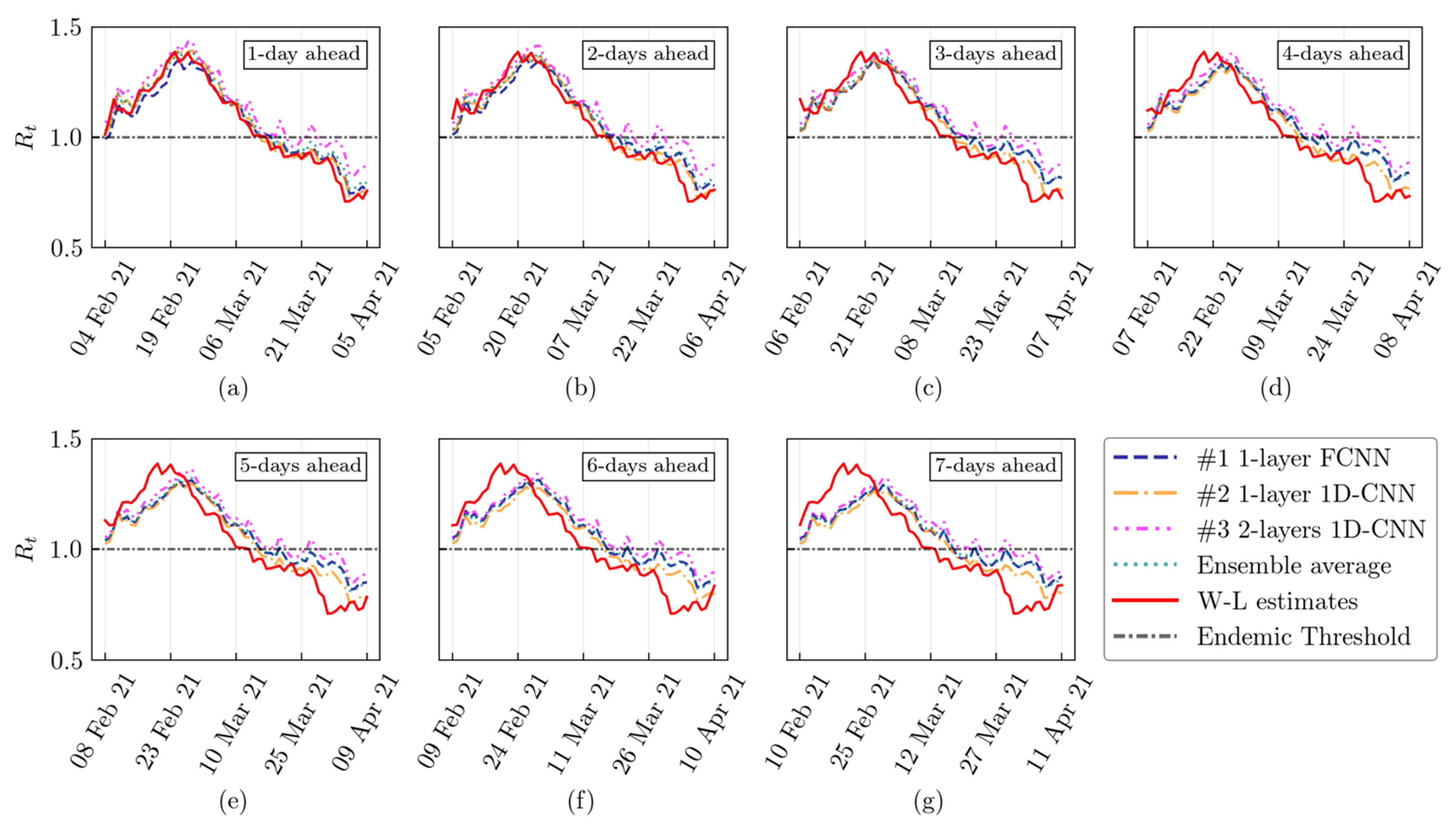
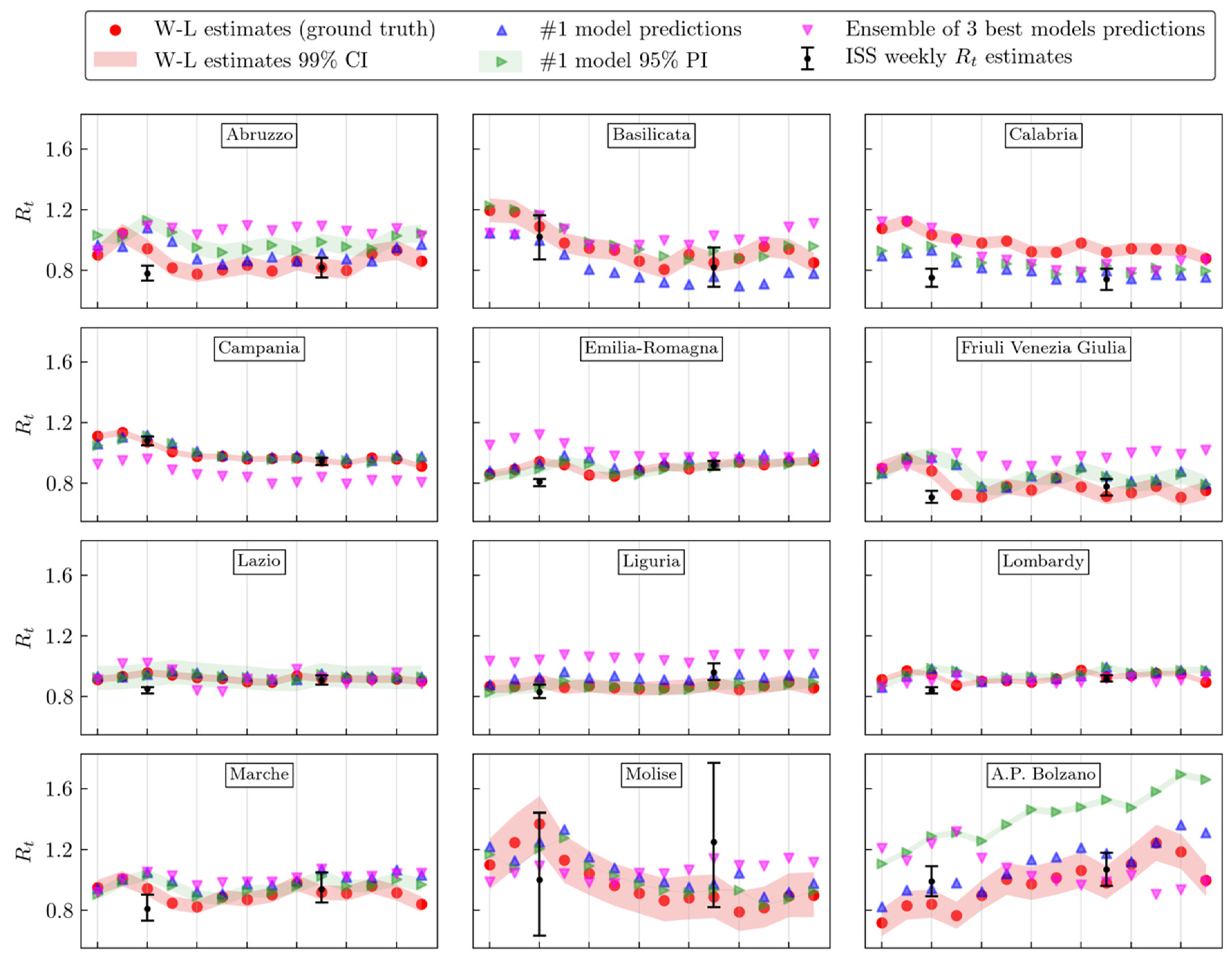
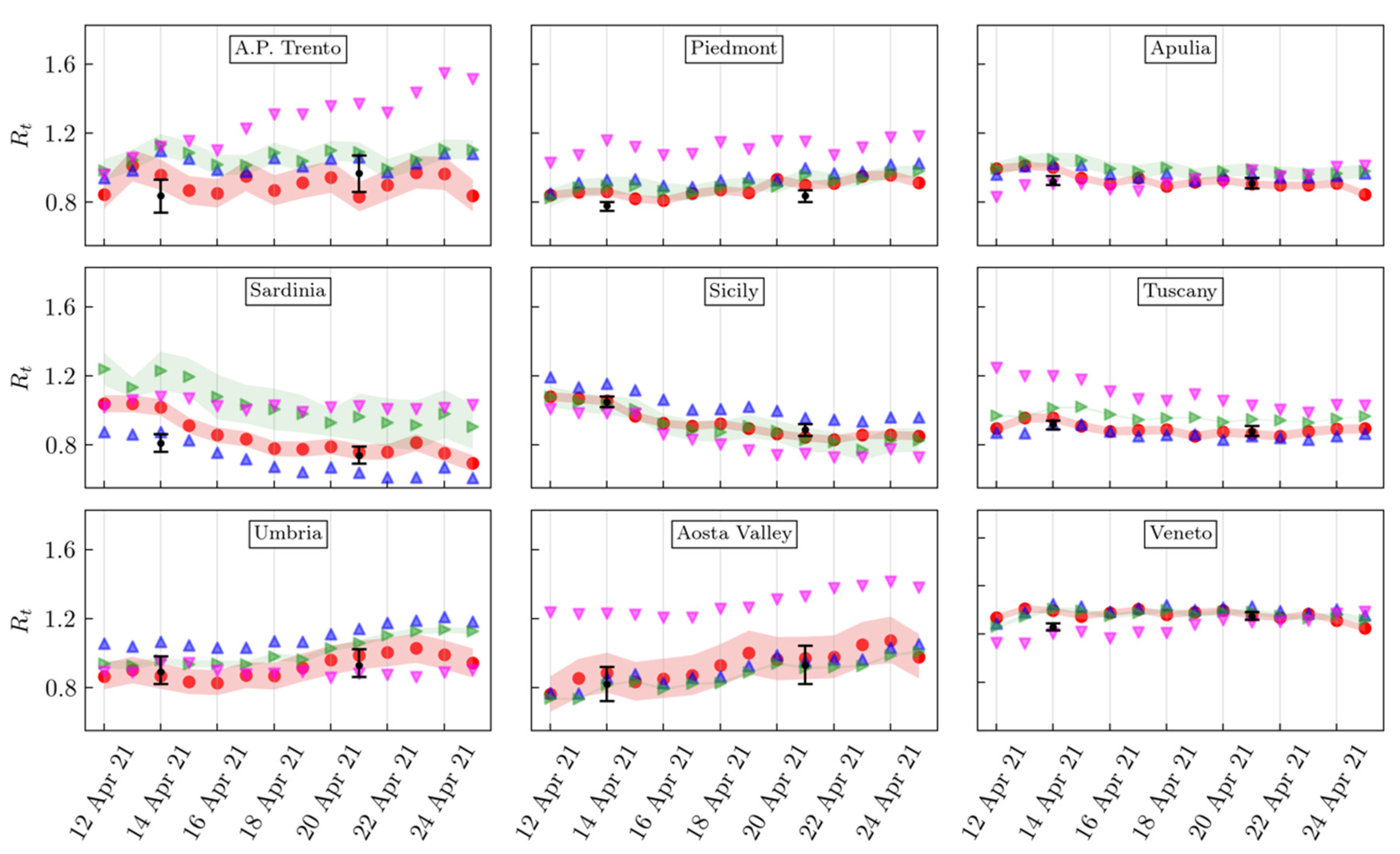
Figure 3 reports the comparison between the test-set Rt ground-truth in Lombardy and the predictions obtained through the three regional best models, which ranked in the top 3 after the K-Fold Cross Validation procedure (#1, #2, and #3, respectively), along with their average ensemble. Specifically, the Rt ground truth was estimated by means of the W–L procedure, as shown in Figure 1. Figure 3 highlights that the prediction error increases as the predicted time grows, leading to inaccurate forecasts for the last instants of the prediction window (from five to seven days ahead). On the contrary, the forecasts obtained for the remaining prediction window time instants (from one to four days ahead) proved to be very accurate. Moreover, it should be noted that considering the three regional best models in the predictive phase is crucial because, as shown in Figure 3, the #2 model (1-layer 1D-CNN) is able to predict the test-set Rt trend better than the #1 model (1-layer FCNN). For each Italian region/autonomous province, the RMSEs evaluated on the test set are reported in Table 3 for each selected architecture and their average ensemble. Figure 4 reports the ground-truth Rt values and the rolling-approach predictions for all the Italian regions and autonomous provinces from 12 to 25 April 2021. The reported predictions were obtained on epidemiological data that were not included in the dataset used for model training, validation, and evaluation procedures, with the aim of evaluating the performance of the proposed framework on new data available daily.
Specifically, for each Italian region or autonomous province, a forecasting phase from 12 to 25 April 2021 exploited the best model (#1) resulting from the K-Fold Cross Validation procedure as well as the average ensemble of the three best-ranked models after the aforementioned procedure. In this phase, the predictions obtained from the models were compared with the W–L Rt estimates (ground truth) and the weekly ISS Rt estimates, as reported in Figure 4. Moreover, Figure 4 also reports the 95% PI of the best model computed as described by Algorithm 2 in Section 2.3. As shown in Figure 4, the proposed framework provides accurate predictions in all the Italian regions and autonomous provinces. In particular, in most regions, all three models proved to be very accurate because their predictions turned out to be very close to the W–L estimates. On the contrary, in some regions, not all models provided accurate forecasts, meaning that some Rt patterns were only learned by specific architectures.

4. Discussion

The present work aimed to define a framework fully based on ANNs for predicting the COVID-19 effective reproduction number Rt in all the Italian regions and autonomous provinces. This indicator is crucial because its value denotes the status of an epidemic (i.e., spread or containment phases), thus allowing policymakers to act in a timely and targeted manner to tackle new outbreaks. In particular, out of the six proposed models, the proposed framework identified three ANNs for each Italian region and autonomous province, which turned out to be optimal for the seven-day ahead prediction of the Rt trend, starting from a daily updated set of 21 epidemiological variables given at a generic day, t. As reported in Section 3, the proposed framework succeeds in the predictive task nationwide, with a prediction error that increases as the prediction time window grows. However, as shown in Table 3, the predictions accuracy varies from territory to territory, meaning that different Rt trends were observed in the Italian country due to the heterogeneous spread of the pandemic. Focusing on Lombardy, which is the region where COVID-19 was more widespread, the predictions obtained through the proposed approach proved to be very accurate, as shown in Figure 3, with a minimum RMSE (on the Rt scale) ranging from 0.035 at day t + 1 to 0.106 at day t + 7. However, because Italian epidemiological data are communicated daily by the ICPD [21], a rolling approach was proposed in order to obtain the most accurate predictions possible at any day to be predicted (Section 2.4), thus improving the prediction accuracy of the models by updating each forecast as soon as new epidemiological data become available. Figure 4 highlights the high level of accuracy of the forecasts produced by the suggested rolling approach for each Italian region and autonomous province. Specifically, it should be noted that, for some regions, not all three models selected for the inference phase produced accurate predictions, meaning that particular trends were learned during the training phase by different architectures. For this reason, the proposed approach does not only rely on a single predictive model, but it also exploits three different ANN architectures in order to maximize the possibility of predicting heterogeneous and complex Rt trends. Notice that the proposed approach allows the forecast of the Rt trend at a daily temporal resolution, whereas official Rt data are currently communicated with a weekly temporal resolution. Forecasts at a finer (daily) temporal resolution could be crucial in a pandemic context, because they could help track the spread of the disease more effectively by rapidly identifying new outbreaks or sudden growth trends. Furthermore, it should be pointed out that traditional statistical methods for estimating the Rt index, typically based on Bayesian approaches, require the observation of epidemiological indicators in a time window whose dimension defines the accuracy of the estimates: the greater the time window, the more accurate the obtained estimates (Section 2.1.1). The proposed framework aims to overcome this limitation by proposing a multivariate approach that exploits the information of different variables at a given day to produce accurate forecasts for the subsequent 7 days. Moreover, it is important to consider that, since 3 November 2020, different containment measures have been applied in Italian regions and autonomous provinces by identifying three pandemic risk scenarios related to increasing critical levels (yellow, orange, and red) [5]. Each risk scenario is based on a weekly evaluation of a set of epidemiological parameters, including the effective reproduction number, Rt, and the number of regional hospitalizations. Therefore, it is important to highlight that the proposed framework could be exploited to predict not only the daily effective reproduction number, but also other epidemiological variables, such as the number of COVID-19 hospitalizations, by simply redefining the target variable in the model training, validation, and testing procedures. In this way, accurate predictions regarding several epidemiological indicators could be obtained in order to facilitate the timely assignment of each territory to the proper risk level in a cost-effective manner. This approach presents some limitations. First, it should be noted that, as expected, an increasing prediction error was observed as the prediction time window increased. For this reason, when possible, the rolling approach should be adopted in order to improve prediction accuracy. When no updated data are available, predictions cannot be updated, leading to a greater prediction error, which varies from territory to territory, as reported in Table 3. Second, consider that the training procedures were conducted by exploiting publicly available data that are regularly revised and updated, thus including an error bias that could be reduced by exploiting more reliable official data. Last, because no official data were available daily regarding the regional effective reproduction number, Rt, the setup of the supervised learning problem required the estimation of the daily ground-truth by means of the Wallinga–Lipsitch algorithm, as described in Section 2.1.1.

5. Conclusions

The present work proposes a framework to forecast the daily R t index 7 days ahead by exploiting a set of 21 epidemiological indicators at a given day, in each Italian region and autonomous province. The obtained predictions were characterized by a finer temporal resolution (daily) compared with the official R t data, which were reported weekly by the Italian National Institute of Health. A finer temporal resolution represents a benefit because the R t is one of the most representative indicators of the infection status. The ANN predictions resulting from the proposed study highlight the fact that accurate forecasts can be achieved for each Italian region and autonomous province, also exploiting the rolling approach procedure that allows the update of the obtained forecasts on a daily basis as soon as new input data become available. For instance, the predictions obtained through the proposed approach in Lombardy, which is a region where COVID-19 was more widespread, proved to be very accurate, with a minimum RMSE (on the Rt scale) ranging from 0.035 at day t + 1 to 0.106 at day t + 7. The proposed framework could be easily rearranged for predicting different epidemiological indicators concerning not only the COVID-19 pandemic, but also other diseases that could potentially appear and spread worldwide. Clearly, this is crucial for containing the disease spread, by imposing timely and appropriate containment measures in order to tackle new outbreaks. As a consequence, the saturation of the health system and the strong impact on the socio-economic fabric could be mitigated because the proposed framework can represent a valid and accurate decision support tool for policy makers.

Author Contributions

Conceptualization, A.G., G.A. (Giovanni Aloisio), G.A. (Gabriele Accarino) and V.A.; methodology, A.G., G.A. (Gabriele Accarino) and V.A.; software, A.G., G.A. (Gabriele Accarino) and V.A.; validation, G.A. (Giovanni Aloisio); formal analysis, A.G., G.A. (Giovanni Aloisio), G.A. (Gabriele Accarino), V.A., F.I. and M.C.; investigation, A.G., G.A. (Giovanni Aloisio), G.A. (Gabriele Accarino), V.A., F.I. and M.C.; resources, A.G., G.A. (Gabriele Accarino) and V.A.; data curation, A.G., G.A. (Gabriele Accarino) and V.A.; writing—original draft preparation, A.G., G.A. (Gabriele Accarino) and V.A.; writing—review and editing, G.A. (Giovanni Aloisio); visualization, A.G., G.A. (Gabriele Accarino) and V.A.; supervision, G.A. (Giovanni Aloisio); project administration, G.A. (Giovanni Aloisio); funding acquisition, not applicable. All authors have read and agreed to the published version of the manuscript.

Funding

This research received no external funding.

Institutional Review Board Statement

Not applicable.

Informed Consent Statement

Not applicable.

Data Availability Statement

Publicly available datasets were used in this study. As reported throughout the manuscript, these datasets can be found at the following links: https://github.com/pcm-dpc/COVID-19 (accessed on 26 January 2022).

Acknowledgments

The authors would like to acknowledge Antonio Aloisio for his editing and proofreading work on this paper.

Conflicts of Interest

The authors declare no conflict of interest.

References

  1. Zhu, N.; Zhang, D.; Wang, W.; Li, X.; Yang, B.; Song, J.; Zhao, X.; Huang, B.; Shi, W.; Lu, R.; et al. A novel coronavirus from patients with pneumonia in China, 2019. N. Engl. J. Med. 2020, 382, 727–733. [Google Scholar] [CrossRef] [PubMed]
  2. WHO. Naming the Coronavirus Disease (COVID-19) and the Virus that Causes It. 2020. Available online: https://www.who.int/emergencies/diseases/novel-coronavirus-2019/technical-guidance/naming-the-coronavirus-disease-(COVID-2019)-and-the-virus-that-causes-it (accessed on 26 January 2022).
  3. Guan, W.-J.; Ni, Z.-Y.; Hu, Y.; Liang, W.-H.; Ou, C.-Q.; He, J.-X.; Liu, L.; Shan, H.; Lei, C.-L.; Hui, D.S.C.; et al. Clinical characteristics of coronavirus disease 2019 in China. N. Engl. J. Med. 2020, 382, 1708–1720. [Google Scholar] [CrossRef]
  4. Prime Minister Decree. Further Implementing Provisions of the Decree-Law 23 February 2020, No. 6, with Urgent Measures in Relation to Containment and Management of the Epidemiological Emergency from COVID-19, Applicable throughout the Country. (20A01605) G.U. General Series, no. 64 (In Italian). 11 March 2020. Available online: https://www.trovanorme.salute.gov.it/norme/dettaglioAtto?id=73643 (accessed on 26 January 2022).
  5. Gazzettaufficiale.it. Prime Minister Decree. 3 November 2020. Available online: https://www.gazzettaufficiale.it/eli/id/2020/11/04/20A06109/sg (accessed on 26 January 2022).
  6. Wallinga, J.; Lipsitch, M. How generation intervals shape the relationship between growth rates and reproductive numbers. Proc. R. Soc. B Boil. Sci. 2006, 274, 599–604. [Google Scholar] [CrossRef] [Green Version]
  7. Clement, J.C.; Ponnusamy, V.; Sriharipriya, K.C.; Nandakumar, R. A survey on mathematical, machine learning and deep learning models for COVID-19 transmission and diagnosis. IEEE Rev. Biomed. Eng. 2021, 15, 325–340. [Google Scholar]
  8. Shorten, C.; Khoshgoftaar, T.; Furht, B. Deep learning applications for COVID-19. J. Big Data 2021, 8, 1–54. [Google Scholar] [CrossRef]
  9. Zou, D.; Wang, L.; Xu, P.; Chen, J.; Zhang, W.; Gu, Q. Epidemic Model Guided Machine Learning for COVID-19 Forecasts in the United States. Medrxiv 2020. [Google Scholar] [CrossRef]
  10. Zhou, T.; Liu, Q.; Yang, Z.; Liao, J.; Yang, K.; Bai, W.; Lu, X.; Zhang, W. Preliminary prediction of the basic reproduction number of the Wuhan novel coronavirus 2019-nCoV. J. Evid.-Based Med. 2020, 13, 3–7. [Google Scholar] [CrossRef] [PubMed]
  11. Peirlinck, M.; Linka, K.; Costabal, F.S.; Bhattacharya, J.; Bendavid, E.; Ioannidis, J.P.; Kuhl, E. Visualizing the invisible: The effect of asymptomatic transmission on the outbreak dynamics of COVID-19. Comput. Methods Appl. Mech. Eng. 2020, 372, 113410. [Google Scholar] [CrossRef]
  12. Giuliani, D.; Dickson, M.; Espa, G.; Santi, F. Modelling and predicting the spatio-temporal spread of COVID-19 in Italy. BMC Infect. Dis. 2020, 20, 700. [Google Scholar] [CrossRef] [PubMed]
  13. Gatto, A.; Accarino, G.; Aloisi, V.; Immorlano, F.; Donato, F.; Aloisio, G. Limits of Compartmental Models and New Opportunities for Machine Learning: A Case Study to Forecast the Second Wave of COVID-19 Hospitalizations in Lombardy, Italy. Informatics 2021, 8, 57. [Google Scholar] [CrossRef]
  14. Zheng, N.; Du, S.; Wang, J.; Zhang, H.; Cui, W.; Kang, Z.; Yang, T.; Lou, B.; Chi, Y.; Long, H.; et al. Predicting COVID-19 in China Using Hybrid AI Model. IEEE Trans. Cybern. 2020, 50, 2891–2904. [Google Scholar] [CrossRef]
  15. Deng, Q. Dynamics and development of the COVID-19 epidemic in the United States: A compartmental model enhanced with deep learning techniques. J. Med. Internet Res. 2020, 22, e21173. [Google Scholar] [CrossRef]
  16. Abbasimehr, H.; Paki, R. Prediction of COVID-19 confirmed cases combining deep learning methods and bayesian optimization. Chaos Solitons Fractals 2021, 142, 110511. [Google Scholar] [CrossRef]
  17. Solanki, A.; Singh, T. COVID-19 Epidemic Analysis and Prediction Using Machine Learning Algorithms. In Studies in Systems, Decision and Control; Springer: Berlin/Heidelberg, Germany, 2021; pp. 57–78. [Google Scholar]
  18. Punn, N.; Sonbhadra, S.; Agarwal, S. COVID-19 epidemic analysis using machine learning and deep learning algorithms. medRxiv 2020. [Google Scholar] [CrossRef] [Green Version]
  19. Zeroual, A.; Harrou, F.; Dairi, A.; Sun, Y. Deep learning methods for forecasting COVID-19 time-series data: A comparative study. Chaos, Solitons Fractals 2020, 140, 110121. [Google Scholar] [CrossRef] [PubMed]
  20. Davahli, M.; Fiok, K.; Karwowski, W.; Aljuaid, A.; Taiar, R. Predicting the dynamics of the COVID-19 Pandemic in the United States using graph theory-based neural networks. Int. J. Environ. Res. Public Health 2021, 18, 3834. [Google Scholar] [CrossRef]
  21. Italian Civil Protection Department (ICPD). GitHub Data Repository. 2020. Available online: https://github.com/pcm-dpc/COVID-19 (accessed on 6 May 2021).
  22. Iss.it. Monitoraggio Settimanale—ISS. 2021. Available online: https://www.iss.it/monitoraggio-settimanale (accessed on 9 June 2021).
  23. Cori, A.; Ferguson, N.; Fraser, C.; Cauchemez, S. A new framework and software to estimate time-varying reproduction numbers during epidemics. Am. J. Epidemiol. 2013, 178, 1505–1512. [Google Scholar] [CrossRef] [PubMed] [Green Version]
  24. Iss.it. FAQ sul Calcolo del Rt—ISS. 2021. Available online: https://www.iss.it/coronavirus/-/asset_publisher/1SRKHcCJJQ7E/content/faq-sul-calcolo-del-rt (accessed on 9 June 2021).
  25. Cereda, D.; Manica, M.; Tirani, M.; Rovida, F.; Demicheli, V.; Ajelli, M.; Poletti, P.; Trentini, F.; Guzzetta, G.; Marziano, V.; et al. The early phase of the COVID-19 epidemic in Lombardy, Italy. Epidemics 2021, 37, 100528. [Google Scholar] [CrossRef]
  26. Wallinga, J.; Teunis, P. Different epidemic curves for severe acute respiratory syndrome reveal similar impacts of control measures. Am. J. Epidemiol. 2004, 160, 509–516. [Google Scholar] [CrossRef] [PubMed] [Green Version]
  27. Fine, T. Feedforward Neural Network Methodology; Springer: New York, NY, USA, 2005. [Google Scholar]
  28. Kiranyaz, S.; Avci, O.; Abdeljaber, O.; Ince, T.; Gabbouj, M.; Inman, D. 1D convolutional neural networks and applications: A survey. Mech. Syst. Signal Process. 2021, 151, 107398. [Google Scholar] [CrossRef]
  29. Kiranyaz, S.; Ince, T.; Abdeljaber, O.; Avci, O.; Gabbouj, M. 1-D convolutional neural networks for signal processing applications. In Proceedings of the IEEE International Conference on Acoustics, Speech and Signal Processing (ICASSP), Brighton, UK, 12–17 May 2019. [Google Scholar]
  30. Hochreiter, S.; Schmidhuber, J. Long Short-Term Memory. Neural Comput. 1997, 9, 1735–1780. [Google Scholar] [CrossRef] [PubMed]
  31. Pascanu, R.; Mikolov, T.; Bengio, Y. On the difficulty of training recurrent neural networks. arXiv 2012, arXiv:1211.5063v2. [Google Scholar]
  32. Bengio, Y.; Simard, P.; Frasconi, P. Learning long-term dependencies with gradient descent is difficult. IEEE Trans. Neural Netw. 1994, 5, 157–166. [Google Scholar] [CrossRef]
  33. Keras. Keras: The Python Deep Learning API. Available online: https://keras.io/ (accessed on 26 January 2022).
  34. Abadi, M.; Agarwal, A.; Barham, P.; Brevdo, E.; Chen, Z.; Citro, C.; Corrado, G.S.; Davis, A.; Dean, J.; Devin, M.; et al. Tensorflow: Large-scale machine learning on heterogeneous distributed systems. arXiv 2016, arXiv:1603.04467. [Google Scholar]
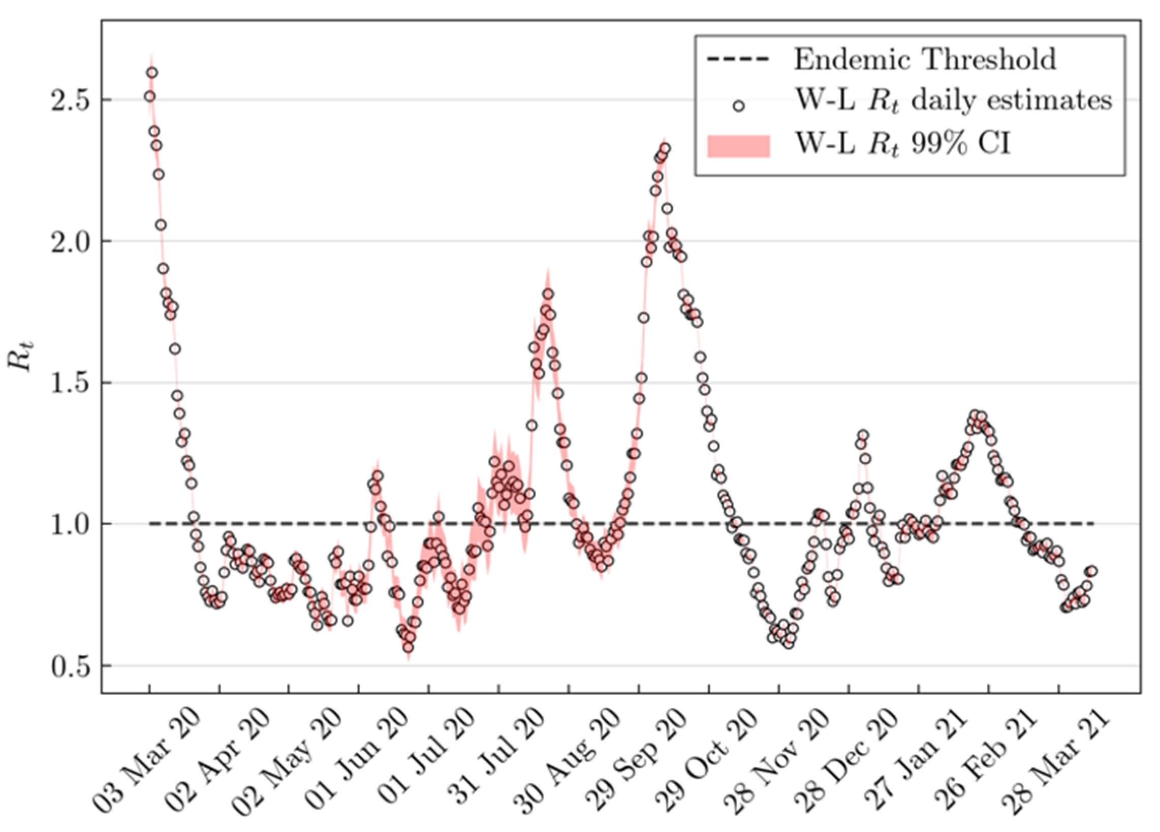
Figure 1. Wallinga–Lipsitch estimates. Wallinga–Lipsitch Rt estimates in Lombardy (black circles) and their 99% CI (red shape) from 3 March 2020 to 11 April 2021. The endemic threshold, corresponding to Rt = 1, is depicted through a dashed black line.
Ai 03 00009 g001
Figure 2. Rolling Approach. The seven-day ahead predictions corresponding to a specific input day, t, are shown in rectangular boxes, whose color determines prediction accuracy. Red circles identify the selected forecasts that will be the output of the framework.
Ai 03 00009 g002
Figure 3. Lombardy Model evaluation. Predictions obtained by means of the regional three best models and their average ensemble model are compared with Wallinga–Lipsitch Rt estimates in the period from 4 February 2021 to 11 April 2021. The endemic threshold (Rt = 1) is also reported.
Ai 03 00009 g003
Figure 4. Effective reproduction number forecasts. Rt rolling forecasts in each Italian region/autonomous province compared with the W–L Rt ground truth (red circles and red region) and with the weekly ISS Rt estimates (black error bars) from 12 to 25 April 2021. The regional best model predictions are represented by blue triangles, whereas the forecasts obtained from the average ensemble of the three models, which ranked in the top 3 after the K-Fold Cross Validation procedure, are reported in the magenta triangles. The 95% Prediction Interval of the best model was also reported (green triangles and green region).
Ai 03 00009 g004aAi 03 00009 g004b
Table 1. Design details of the models.
Model1-Layer
FCNN
2-Layers
FCNN
1-Layer
1D-CNN
2-Layers
1D-CNN
1-Layer
LSTM
2-Layers
LSTM
#Units (per layer)4221; 21--4221; 21
#Filters (per layer)--2110; 10--
Kernel size (per layer)--11; 1--
Stride (per layer)--11; 1--
Activation function
(per layer)
ReLUReLU;
ReLU
SigmoidReLU;
ReLU
TanhTanh;
Tanh
Weights Regularizer
(per layer)
L1 (0.001)L1 (0.01);
L1 (0.01)
L1 (0.001)L1 (0.001);
L1 (0.001)
L1(0.001)/L2(0.01)L1 (0.001)/L2(0.01);
L1 (0.001)/L2(0.01)
Bias Regularizer
(per layer)
L1 (0.001)L1 (0.01);
L1 (0.01)
L1 (0.001)L1 (0.001);
L1 (0.001)
L1(0.001)/L2(0.01)L1(0.001)/L2(0.01);
L1 (0.001)/L2(0.01)
Weights Initializer
(per layer)
UniformUniform; UniformUniformUniform;
Uniform
GlorotUniform; Uniform
Bias Initializer
(per layer)
UniformUniform; UniformUniformUniform;
Uniform
GlorotUniform; Uniform
ReLU = Rectified Linear Unit, L1 = Lasso Regularization, Tanh = Hyperbolic Tangent, Sigmoid = Sigmoid Function, Glorot = Glorot Uniform initializer, FCNN = Fully Connected Neural Network, 1D-CNN = Mono-Dimensional Convolutional Neural Network, LSTM = Long Short–Term Memory.
Table 2. Fitting parameters of the models.
Model1-Layer
FCNN
2-Layers
FCNN
1-Layer 1D-CNN2-Layers 1D-CNN1-Layer LSTM2-Layers
LSTM
Batch Size442244
Learning Rate0.00010.00010.00010.00010.0010.001
Decay Rate0.90.90.90.90.90.9
Loss Early Stopping (patience)505050505050
Validation Loss Early Stopping (patience)505050505050
Epochs400040004000400040004000
ShuffleTrueTrueTrueTrueFalseFalse
FCNN = Fully Connected Neural Network, 1D-CNN = Mono-Dimensional Convolutional Neural Network, LSTM = Long Short–Term Memory.
Table 3. Regional RMSE on the test set for the top three architectures.
RegionArchitecturef(t + 1)
RMSE
f(t + 2)
RMSE
f(t + 3)
RMSE
f(t + 4)
RMSE
f(t + 5)
RMSE
f(t + 6)
RMSE
f(t + 7)
RMSE
Abruzzo1-L FCNN0.0710.1130.1440.1720.2210.2490.252
1-L 1D CNN0.080.1040.0830.1090.0950.110.106
2-Ls 1D CNN0.1070.1130.1190.1140.120.1210.117
Ensemble0.0850.1090.1130.1310.1420.1570.156
Aosta Valley1-L FCNN0.1010.1130.1370.1550.1630.1580.149
1-L 1D CNN0.1370.1280.1510.1610.1670.1630.162
2-Ls 1D CNN0.1370.130.1440.1630.1750.1720.177
Ensemble0.1190.1210.1420.1590.1680.1640.162
Apulia1-L FCNN0.0430.0590.0650.0750.0830.0860.09
2-Ls 1D CNN0.0980.0940.0980.0980.1070.1050.111
1-L 1D CNN0.0940.1010.0810.1010.110.1150.115
Ensemble0.0750.0810.0790.0890.0980.10.104
Basilicata1-L LSTM0.1360.1340.1320.1370.1440.1660.179
1-L FCNN0.0660.0950.1150.1430.1720.2060.217
1-L 1D CNN0.0660.0910.1050.1240.1380.1650.178
Ensemble0.0780.1010.1150.1340.1490.1760.187
Calabria1-L LSTM0.1340.1590.1770.1920.2090.2220.225
1-L FCNN0.0640.0960.1190.1390.1630.1870.187
2-Ls 1D CNN0.120.120.110.1070.1070.1130.105
Ensemble0.1050.1240.1340.1440.1580.1710.169
Campania1-L FCNN0.0320.0520.0650.0720.0810.0880.094
2-Ls 1D CNN0.0320.0550.0670.0720.080.0910.093
1-L 1D CNN0.0320.0540.0650.0730.0830.0930.098
Ensemble0.0310.0530.0660.0720.0810.0910.095
Emilia-Romagna1-L FCNN0.0270.0380.0430.0490.060.0690.077
2-Ls 1D CNN0.0660.090.1120.1340.160.180.198
1-L 1D CNN0.0250.0390.0430.0570.0730.0840.093
Ensemble0.0310.0420.0530.0650.0810.0950.107
Friuli Venezia Giulia1-L FCNN0.0720.1080.1490.1780.2090.2290.237
1-L 1D CNN0.0740.1080.1360.180.2070.2140.238
2-Ls 1D CNN0.150.1790.20.2460.2850.2860.309
Ensemble0.0960.130.1610.20.2330.2430.261
Lazio1-L FCNN0.0260.040.0520.0620.0740.0850.092
2-Ls 1D CNN0.1670.1680.1730.1730.1650.1630.167
1-L 1D CNN0.1150.1390.1270.1080.1230.1120.124
Ensemble0.0980.1050.1030.0980.10.0960.103
Liguria1-L FCNN0.0610.0830.1040.1180.1310.1480.162
1-L 1D CNN0.0350.0480.0650.0790.0920.1020.11
2-Ls 1D CNN0.0390.0670.0770.0890.1010.1150.126
Ensemble0.040.0610.0780.0920.1060.1190.13
Lombardy1-L FCNN0.0410.0590.0770.0880.0990.1080.117
1-L 1D CNN0.0350.0480.0610.0690.0830.0960.106
2-Ls 1D CNN0.0840.0930.1010.1090.1180.1290.138
Ensemble0.0460.0620.0770.0850.0970.1080.118
Marche1-L FCNN0.0670.1010.1370.1560.1810.2070.22
2-Ls 1D CNN0.1850.1770.1510.1440.1550.1450.149
2-Ls FCNN0.0450.0640.0780.10.1170.1280.137
Ensemble0.0910.1070.1180.1310.1480.1560.164
Molise1-L LSTM0.0970.1120.1280.1330.1420.1440.15
1-L FCNN0.0910.0980.1210.120.1230.1180.136
1-L 1D CNN0.0920.1190.1360.1460.1550.1670.18
Ensemble0.0930.1080.1270.1310.1390.1410.154
Piedmont1-L FCNN0.0610.0830.0920.1180.120.1360.151
1-L 1D CNN0.0370.0510.0650.0710.0790.0860.092
2-Ls 1D CNN0.0690.0870.1010.1150.1310.140.144
Ensemble0.0450.0630.0740.0880.0990.1090.116
Sardinia1-L FCNN0.1580.2130.2330.2520.2860.3150.346
1-L 1D CNN0.070.0930.1220.1470.1750.1990.217
2-Ls 1D CNN0.0910.1190.1540.1820.2050.2340.261
Ensemble0.080.1230.1560.1820.2120.240.266
Sicily1-L FCNN0.0540.0760.0920.1120.1180.1290.128
2-Ls 1D CNN0.1880.2270.2310.2320.2260.2190.224
1-L 1D CNN0.0680.0520.0550.0570.060.0650.079
Ensemble0.0980.1080.1150.1190.1170.1160.108
A.P. Bolzano1-L FCNN0.080.1370.1730.1840.2070.2150.232
2-Ls 1D CNN0.1410.2290.2980.3670.4060.4550.462
2-Ls FCNN0.1720.1820.1910.1970.2050.2110.217
Ensemble0.1270.180.2180.2450.2680.2880.298
A.P. Trento1-L FCNN0.0770.0970.1130.130.1410.1540.158
2-Ls 1D CNN0.210.2380.2640.2940.3090.3320.353
1-L 1D CNN0.0810.1030.1270.1450.1710.1840.196
Ensemble0.1110.1360.1590.1810.1990.2180.23
Tuscany1-L FCNN0.0480.0530.0570.0630.0720.0760.08
2-Ls 1D CNN0.050.0560.0730.0820.1050.0850.088
1-L 1D CNN0.0480.0510.0550.0720.0670.0760.08
Ensemble0.030.0410.0470.0560.0670.0670.069
Umbria1-L FCNN0.0780.1280.160.1780.2240.2340.249
2-Ls 1D CNN0.1190.1220.1190.1210.1210.1190.116
1-L LSTM0.3650.3910.4110.4150.4350.4330.434
Ensemble0.1680.1990.2170.2270.2460.2480.254
Veneto1-L FCNN0.0660.0850.1060.1340.1550.1750.185
2-Ls 1D CNN0.1430.1450.1560.1610.170.1810.19
1-L 1D CNN0.0870.0940.10.1080.1250.1350.141
Ensemble0.0950.1050.1190.1320.1490.1610.168
A.P. = Autonomous Province, RMSE = Root Mean Squared Error, 1-L FCNN = 1 Layer Fully Connected Neural Network, 1-L 1D CNN = 1 Layer Mono-Dimensional Convolutional Neural Network, 1-L LSTM = 1 Layer Long Short-Term Memory, 2-Ls FCNN = 2 Layers Fully Connected Neural Network, 2-Ls 1D CNN = 2 Layers Mono-Dimensional Convolutional Neural Network.
Publisher’s Note: MDPI stays neutral with regard to jurisdictional claims in published maps and institutional affiliations.