DeepSleep 2.0: Automated Sleep Arousal Segmentation via Deep Learning

Abstract

DeepSleep 2.0 is a compact version of DeepSleep, a state-of-the-art, U-Net-inspired, fully convolutional deep neural network, which achieved the highest unofficial score in the 2018 PhysioNet Computing Challenge. The proposed network architecture has a compact encoder/decoder structure containing only 740,551 trainable parameters. The input to the network is a full-length multichannel polysomnographic recording signal. The network has been designed and optimized to efficiently predict nonapnea sleep arousals on held-out test data at a 5 ms resolution level, while not compromising the prediction accuracy. When compared to DeepSleep, the obtained experimental results in terms of gross area under the precision–recall curve (AUPRC) and gross area under the receiver operating characteristic curve (AUROC) suggest a lightweight architecture, which can achieve similar prediction performance at a lower computational cost, is realizable.

1. Introduction

Sleep is an important element of our daily life, affecting our health and quality of life. Estimates [1] suggest that 34.8% of the adult population in the United States suffer from insufficient sleep (less than 7 h in 24 h). Similarly, about 50 to 70 million of the population suffers from wakefulness and various types of sleep disorders [2]. Inadequate sleep may be linked to a wide range of negative outcomes including cardiovascular dysfunction, obesity, depression, hypotension, irritability, impaired memory, and learning issues [3,4]. Sleep disorders often track their roots to some type of sleep disturbance. Sleep disturbances are of various nature. For instance, obstructive sleep apnea (or simply, apnea), characterized by a complete collapse of the airway, leads to awakening and subsequent sleep disturbance.

While apneas are one of the most common sleep disturbances, they are certainly not the only ones. Sleep arousals, defined as brief intrusions of wakefulness into sleep [5], can occur spontaneously as a result of sleep-disordered breathing (e.g., partial airway obstructions or snoring) or other sleep disorders. Each arousal, lasting 3 to 15 s, triggers a lighter sleep stage. Humans are usually not aware of sleep arousals; however, they might be aware of awakenings (sleep arousals lasting more than 15 s). Sleep quality will deteriorate with the frequent occurrence of sleep arousals. For instance, according to the American Sleep Apnea Association (ASAA), as few as five arousals per hour can make someone feel chronically sleepy. Symptoms resulting from frequent sleep arousals are sympathetic activation, nonrestorative sleep, and daytime sleepiness [4]. While apnea is one of the better-studied sleep disorders [3], there are only a few studies related to sleep arousals. The main reasons are expensive research due to the difficulties associated with sleep arousal detection with traditional methods and, compared with apnea, automated detection of such sleep arousals has been shown to have low scoring reliability [6].

Early detection of excessive sleep arousals is essential for the diagnosis and treatment of sleep disorders. Early diagnosis might help reduce the risk of potential complications, including blood pressure fluctuations and heart disease. The current state-of-the-practice (gold standard) in sleep arousal detection consists of human-annotated multichannel polysomnographic (PSG) recordings. Traditionally, 30 s epochs of PSG recordings are visually inspected and labeled by certified sleep experts according to the American Academy of Sleep Medicine’s (AASM) scoring manual [7]. This task requires considerable time and effort as the amount of data to inspect is tremendous. For instance, an 8 h and 13-channel sleep recording sampled at 200 Hz contains almost 75 million data points. It may take hours to manually score a sleep recording of this scale. Moreover, the overall inter-rater consensus for the AASM standard is only about 80% [2]. Hence, the development of more efficient and more consistent methods is of high importance.

The main aim of this paper is to realize an efficient and automatic nonapnea sleep arousal segmentation method based on deep learning methods. A fully convolutional neural network (CNN) with a compact encoder–decoder structure is proposed together with various types of preprocessing, data augmentation, and training strategies. The best-performing variant of the trained model is compared to the current state-of-the-art method in various ways.

The structure of this paper is as follows: Section 2 provides the necessary background on mathematical modeling and discusses some related works. The underlying dataset is introduced and analyzed in Section 3. The proposed CNN architecture is presented in Section 4 and the obtained experimental results are given in Section 5. Finally, concluding remarks are provided in Section 7.

2. Background

2.1. Problem Formulation

Let $\mathit{x}\in {\mathbb{R}}^{C\times S}$ be a signal (e.g., a PSG sleep record) with $C\in {\mathbb{Z}}^{+}$ physiological channels and a total length of $S=T/\Delta t$ data points. Here, $T\in {\mathbb{Z}}^{+}$ stands for the total length of the recorded signal in seconds and $\Delta t>0$ is the per-second sampling resolution. The aim is to find a model $f\left(\mathit{x},\mathit{\theta }\right)$ which maps the input signal $\mathit{x}$ into the prediction space $\widehat{\mathit{y}}=\left[{\widehat{y}}_1,\dots ,{\widehat{y}}_S\right]\in {\mathbb{R}}^S$. Here, ${\widehat{y}}_i$ corresponds to a predicted sleep arousal probability, i.e., ${\widehat{y}}_i\in [0,1]$, or to a sleep arousal state, i.e., ${\widehat{y}}_i\in \{0,1\}$, at time instance $t_i=i\Delta t$, and is associated with ${\mathit{x}}_i\in {\mathbb{R}}^C$, a slice from the overall recording signal $\mathit{x}=\left[{\mathit{x}}_1,\dots ,{\mathit{x}}_i,\dots ,{\mathit{x}}_S\right]$. Similarly, $i\in \mathcal{R}$ is a discrete time instance and $\mathcal{R}=\{1,\dots ,S\}$ represents a set of all discrete time instances of the record $\mathit{x}$.

The problem described in this section is also known as sleep segmentation and can be mathematically defined as an optimization problem:

$$\underset{\mathbf{\theta }}{min}\mathcal{D}\left(\widehat{\mathit{y}}-\mathit{y}\right),$$

(1)

subject to

$$\widehat{\mathit{y}}=f\left(\mathit{x},\mathbf{\theta }\right).$$

(2)

Here, $\mathit{y}\in {\mathbb{R}}^S$ represents the vector of true labels, i.e., the expert-segmented signal for the presence of nonapnea arousals; $\mathcal{D}(·)$ is some distance measure; $f\left(·\right)$ is, in general, a nonlinear function, hereafter referred to as model, which maps the input space ${\mathbb{R}}^{C\times S}$ to the target sleep arousal space, i.e., ${\mathbb{R}}^{C\times S}\to {\mathbb{R}}^S$. The set of parameters defining the mapping function is denoted by $\mathbf{\theta }$. In this work, $f\left(·\right)$ is constructed using a deep neural network architecture and $\mathcal{D}$ is approximated by a binary cross-entropy (BCE) loss function for model training purposes.

From the deep learning perspective, the problem can be formulated as a nonapnea sleep arousal classification (i.e., arousal/nonarousal) or as a continuous prediction problem (i.e., arousal probability). The aim is to use the inherent patterns from the available PSG signals to correctly classify or predict target arousal regions. The classification problem will be considered as a benchmark case as target labels are usually available for it (i.e., expert labeled arousal/nonarousal recordings). The prediction problem can be viewed as an extension or potential use-case of the final, trained, model.

2.2. Related Works

One of the first steps in sleep disorders diagnosis is sleep stage classification. There has been a great deal of attention in developing computational methods for automatic sleep staging based on PSG recordings and/or radiofrequency (RF) signals. Neural-network-based approaches tend to greatly outperform “classical” machine learning (ML) methods such as logistic regression, random forest, and support vector machines (SVMs). Particularly, deep learning techniques such as CNN and recurrent neural network (RNN), or their combination, show very good results in sleep stage classification, see [8] for RF-signal-based and [8,9,10,11,12,13,14] for PSG-signal-based approaches.

When it comes to sleep disorders detection, the majority of published works is dedicated to apnea detection. Apnea can be relatively easily detected from the rapid fall in the blood oxygen saturation level. However, changes in physiological signals are very subtle when sleep arousals occur. This is one of the reasons why some researchers argue that automatic sleep arousal segmentation is considerably more challenging than sleep stage scoring [4]. Early works in sleep arousal detection include standard signal processing techniques for feature extraction and subsequent label classification using standard classifiers, such as SVM, Fisher’s linear and quadratic discriminants, and simple feedforward neural networks [15]. State-of-the-art signal processing methods designed for automatic sleep stage scoring, such as short-time Fourier transform (STFT) or Thomson’s multitaper, were shown in [4] to not be well-suited when adopted and applied to an arousal detection problem.

The 2018 “You Snooze, You Win” PhysioNet Computing in Cardiology Challenge [3] triggered a great deal of interest in developing ML-based computational methods for automatic sleep arousal detection. Among the first ten highest scored submissions in the PhysioNet challenge, the last two submissions employed classical ML techniques [9,16], while the remaining eight employed a variant of deep neural networks. Particularly, four models employed a pure CNN method [4,17,18,19], two used the pure RNN method [20,21], while two submissions leveraged both CNN and RNN methods [22,23]. Interestingly enough, the highest scored submission [4] leveraged pure CNN, while the second-highest score was achieved by a combination of CNN and RNN techniques [22].

The trend of leveraging CNN and/or RNN techniques remained present also in works investigated in the follow-up phase of the 2018 challenge, see the recent review paper by Qian et al. [24]. For instance, the originally proposed hybrid scattering transform—bidirectional long short-term memory (BiLSTM) network [21]—was extended in [25]. The authors leveraged four different neural layer types: a second-order ST with Morlet wavelets, convolutional layers, BiLSTM layers, and dense layers. A classification through multiple CNN layers and a random forest module for ensemble voting was proposed in [26]. A comparative study of five recent state-of-the-art CNN models for sleep arousal detection, originally devised for image or speech processing applications, was presented in [27]. A lightweight CNN architecture has recently been proposed in [28] for downsampled and nonoverlapping windowed segments of PSG signals. The authors used a special data augmentation technique to improve the large class imbalance ratio.

3. Data

3.1. Data Source

The underlying data considered in this work were made publicly available for the You Snooze You Win - The PhysioNet Computing in Cardiology Challenge 2018, hereafter referred to as the PhysioNet dataset. In this challenge, computational methods were evaluated for predicting nonapnea sleep arousals on large unseen test data.

The PhysioNet dataset includes 1983 unique subjects with an average age of 55 years and a 65% male population. The data are split into a training set ($n=994$) and test set ($n=989$). With a Kolmogorov–Smirnov test p-value of 0.97, the data were partitioned in a balanced way to ensure a uniform distribution of apnea-hypopnea indices in both sets [3].

The arousal labels for the test dataset ($n=989$ records) were retained for the challenge purposes and were not released to the public after the competition. Therefore, only the complete (containing both recordings and labels) training dataset ($n=994$ records) is considered in this work. The dataset and the challenge are described in more detail in [3]. For completeness, some important aspects are recalled and further analyzed below.

3.2. Data Description

Each record in the dataset contains 13 physiological measurements, including six-channel electroencephalography (EEG) at F3-M2, F4-M1, C3-M2, C4-M1, O1-M2, and O2-M1; one single-channel electrooculography (EOG) at E1-M2; three-channel electromyography (EMG) of the chin, abdominal (ABD), and chest movements; one measurement of respiratory airflow; one measurement of oxygen saturation (SaO${}_2$); and one single-lead electrocardiogram (ECG).

All PSG recordings were measured in microvolts and collected by technicians following the AASM standards. Except for SaO${}_2$, all signals were sampled at a resolution of 5 ms (1/200 Hz = 5 ms). To synchronize the measurements, the SaO${}_2$ was upsampled using a sample and follow method to 200 Hz and was expressed as a percentage. Subsequently, certified sleep technologists annotated each recording for the presence of arousals interrupting the sleep of the subject [3].

For the PhysioNet challenge purposes, the nonapnea arousals were precomputed and defined as regions, ${\mathcal{R}}_a$, where either of the following conditions were met [3]:

C₁: 

From 2 s before a respiratory-effort-related arousal begins, up to 10 s after it ends or,

C₂: 

From 2 s before a nonrespiratory-effort-related arousal, nonapnea arousal begins, up to 2 s after it ends.

Nonscored regions, ${\mathcal{R}}_{ns}$, were defined as regions falling within 10 s before or after a subject woke up, had a hypopnea arousal, or an apnea arousal (labels marked by $y_i=-1,i\in {\mathcal{R}}_{ns}$). Otherwise, arousal regions were labeled as $y_i=1,i\in {\mathcal{R}}_a$, and nonarousal regions as $y_i=0,i\in {\mathcal{R}}_{na}$, where ${\mathcal{R}}_{na}\triangleq \mathcal{R}\setminus \left({\mathcal{R}}_a\cup {\mathcal{R}}_{ns}\right)$.

3.3. Data Analysis

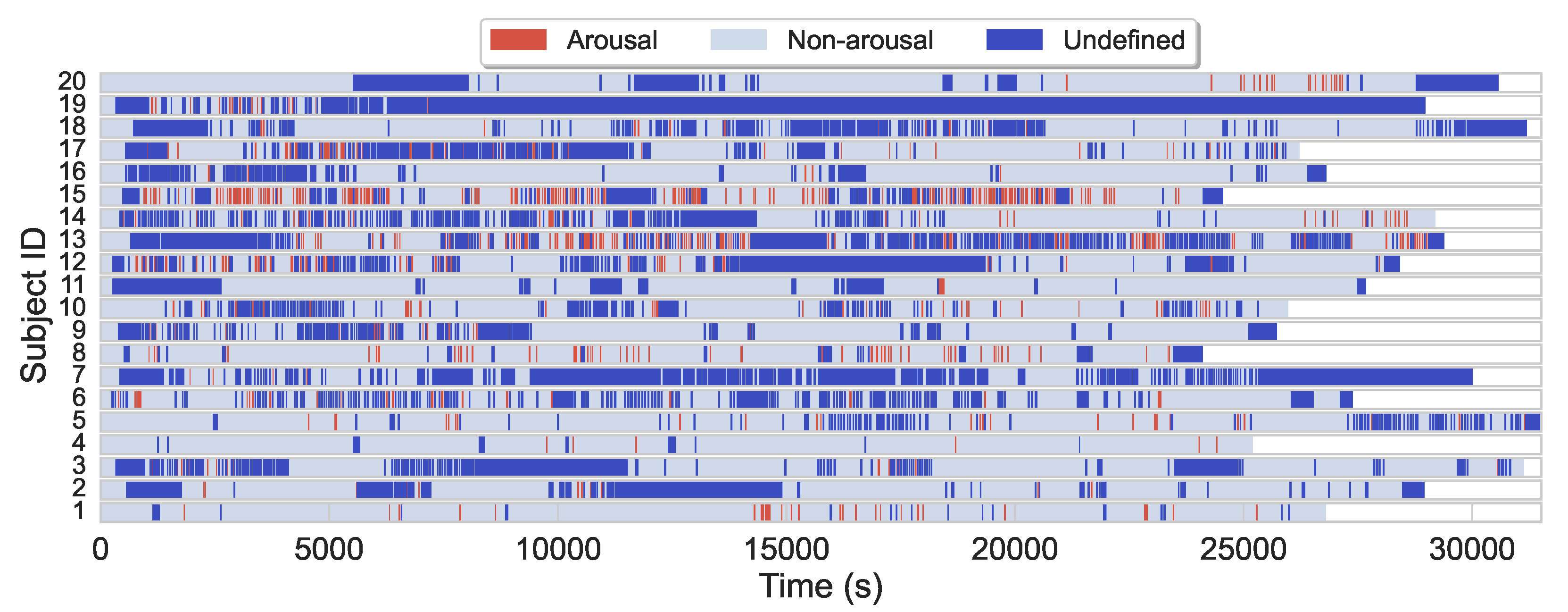
The average sleep duration in the (training) dataset is 7.7 h, while the majority of subjects slept 7–8 h. Arousal regions only account for about 4.6% of the entire dataset, while nonarousal regions and nonscoring regions account for about 61.5% and 33.9%, respectively. Additionally to arousals scarcity, arousals are also often sparsely and heterogeneously distributed during sleep for most subjects, see Figure 1 for illustration.

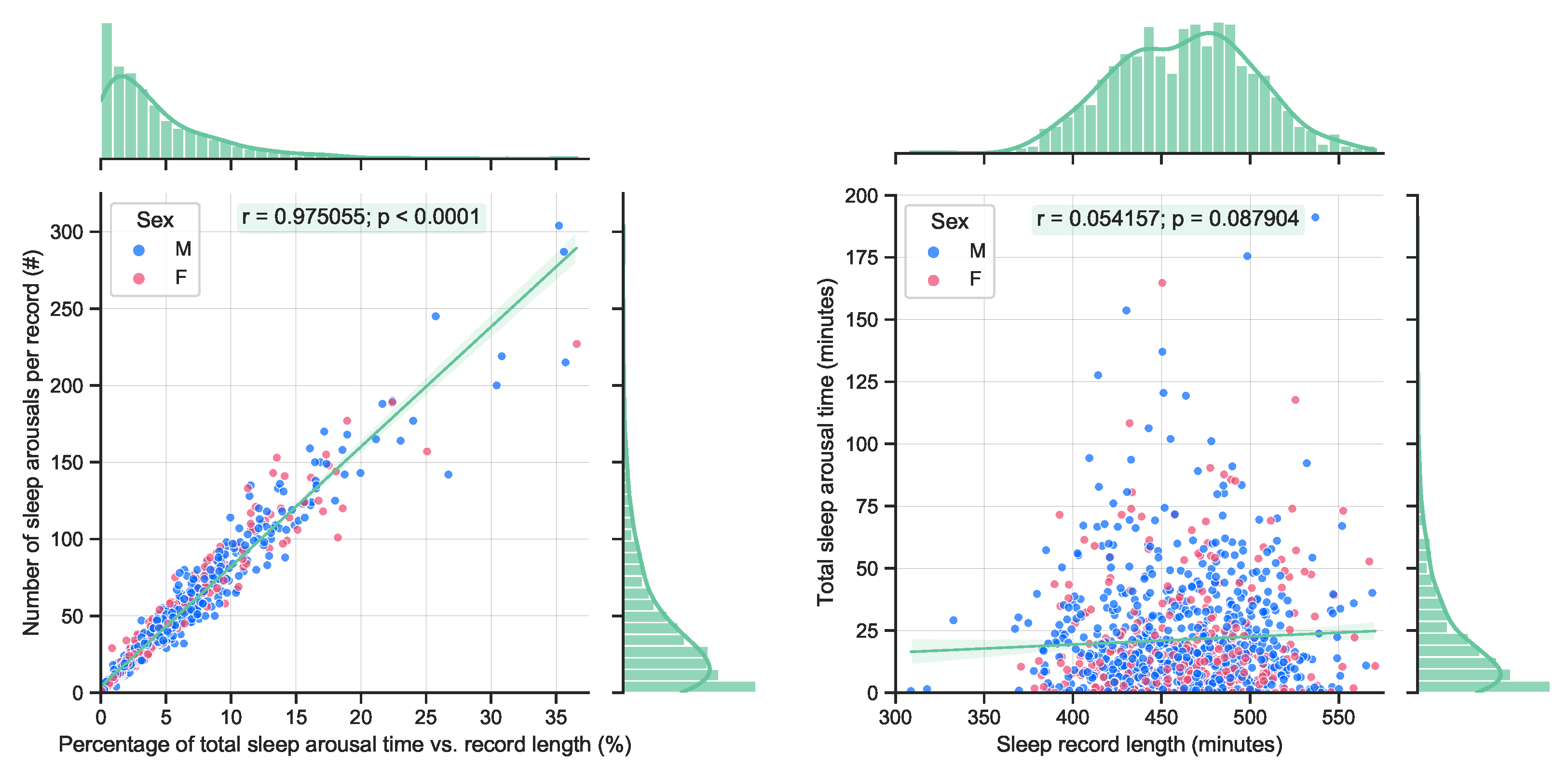
By definition, sleep arousals are short events (less than 15 s). Therefore, it is expected that a longer accumulated arousal time will yield to an increased number of arousal events, see Figure 2 (left). A quite significant correlation can be observed. On the other hand, no significant correlation with the total length of sleep and the accumulated length of sleep arousals can be observed in the available data, see Figure 2 (right). This is also expected, as longer sleep does not necessarily guarantee a better quality of sleep.

All the above-mentioned aspects pose a significant challenge in creating accurate and efficient automatic sleep arousal detection algorithms.

4. Methods

4.1. Network Architecture

The core of the proposed network architecture is inspired by the state-of-the-art DeepSleep architecture. To the author’s knowledge, DeepSleep stands currently as a benchmark for sleep arousal segmentation from PSG signals. Its main building blocks are recalled in the following section.

4.1.1. DeepSleep Architecture

DeepSleep was inspired by the pioneering U-Net [29] architecture which was originally proposed for biomedical image segmentation. DeepSleep is a fully convolutional deep neural network (the authors of DeepSleep concluded that integrating an LSTM or gated recurrent unit into DeepSleep did not improve the performance) for time sleep arousal segmentation. The input to the DeepSleep is a multichannel PSG signal of fixed length $S=2^{23}$, which is then mapped into a dense segmented output in a single forward pass. The key differentiating factor of the DeepSleep architecture is its ability to leverage long-range and short-range interdependencies across different time scales (second, minute, and hours) of the entire sleep record and its ability to detect sleep arousals at the millisecond level.

DeepSleep consists of two modules, an encoder and a decoder module. The encoder module contains several encoder blocks. Each block consists of two convolutional layers with kernel size 7, no kernel dilatation, stride 1, and rectified linear unit (ReLU) activation. The number of output channels increases with each double convolution. A batch normalization follows each convolution. After the double convolution, the signal length is reduced by a max pooling (kernel size 2 or 4, stride 2 or 4). The decoder module is built up of individual decoder blocks. These blocks mirror the encoder blocks’ operation, i.e., each decoder block first performs an upsampling operation (with kernel size 2 or 4 and stride 1) using the so-called transposed convolution. The upscaled signal is then concatenated with the output of the mirrored encoder block. This operation is then followed by a double convolution with the same parameters as above, however, the number of output channels is decreasing this time.

The encoder/decoder blocks are constructed in such a way that the output of the final decoder has the same temporal resolution as the input signal, but contains only one channel. In other words, the encoder and decoder modules map an input signal in ${\mathbb{R}}^{C\times S}$ into an output in ${\mathbb{R}}^S$. Note that the authors of DeepSleep have performed extensive experiments to find the optimal convolutional kernel size, number of encoder/decoder blocks (i.e., shallow vs. deep architecture), max pooling vs. average pooling.

4.1.2. Proposed Architecture

Large parts of the proposed model architecture, hyperparameters, and data augmentation strategies were adopted from its predecessor DeepSleep [4], which was shown to outperform other computational methods in the PhysioNet Challenge. The aim was to leverage the extensive design considerations, supported by exhaustive empirical analyses, in the design of a new lightweight version of DeepSleep, referred to in this work as DeepSleep 2.0. The proposed architecture is illustrated in Figure 3 and its technical backbone is summarized in

Table 1. DeepSleep 2.0 model architecture with $C=13$ physiological channels and input signal centered and padded to a total length of $S=2^{23}=$ 8,388,608 data points.

ID	Layer Type	Output Dimension	Kernel Size	Batch Normalization	Activation Function	Stride	Padding	Weights Initialization
-	Input (symbolic)	$C\times S\phantom{...}$	-	-	-	-	-	-
1	Input	$13\times 2^{23}$	-	-	-	-	-	-
2	Double convolution	$15\times 2^{23}$	7	yes	ReLU	1	same	Xavier
3	Max pooling	$15\times 2^{21}$	4	-	-	4	-	-
4	Double convolution	$30\times 2^{21}$	7	yes	ReLU	1	same	Xavier
5	Max pooling	$30\times 2^{18}$	8	-	-	8	-	-
6	Double convolution	$60\times 2^{18}$	7	yes	ReLU	1	same	Xavier
7	Max pooling	$60\times 2^{14}$	16	-	-	16	-	-
8	Double convolution	$120\times 2^{14}$	7	yes	ReLU	1	same	Xavier
9	Max pooling	$120\times 2^{9\phantom{1}}$	32	-	-	32	-	-
10	Double convolution	$120\times 2^{9\phantom{1}}$	7	yes	ReLU	1	same	Xavier
11	Upsampling	$120\times 2^{14}$	32	-	-	32	-	-
12	Concatenate with ID 8 output	$240\times 2^{14}$	-	-	-	-	-	-
13	Double convolution	$60\times 2^{14}$	7	yes	ReLU	1	same	Xavier
14	Upsampling	$60\times 2^{18}$	16	-	-	16	-	-
15	Concatenate with ID 6 output	$120\times 2^{18}$	-	-	-	-	-	-
16	Double convolution	$30\times 2^{18}$	7	yes	ReLU	1	same	Xavier
17	Upsampling	$30\times 2^{21}$	8	-	-	8	-	-
18	Concatenate with ID 4 output	$60\times 2^{21}$	-	-	-	-	-	-
19	Double convolution	$15\times 2^{18}$	7	yes	ReLU	1	same	Xavier
20	Upsampling	$15\times 2^{23}$	4	-	-	4	-	-
21	Concatenate with ID 2 output	$30\times 2^{23}$	-	-	-	-	-	-
22	Double convolution	$15\times 2^{23}$	7	yes	ReLU	1	same	Xavier
23	Output convolution	$1\times 2^{23}$	1	-	Sigmoid *	1	-	Xavier
-	Output (symbolic)	$1\times S\phantom{...}$	-	-	-	-	-	-
Total trainable parameters: 740,551, parameters memory size: 2.82 (MB)

* The sigmoid activation function is only applied during model inference. During model training, a linear activation is considered and the network outputs logits.

.

The major differences are the number of encoder/decoder blocks. While in the original design, in total ten symmetric encoder/decoder blocks were used, in the proposed compact version, only four blocks are considered. Additionally, the transposed convolution is implemented as a linear interpolation (upsampling in Table 1). The authors of DeepSleep have empirically shown that longer recording lengths lead to better performance. This premise has been strictly adopted in this work and DeepSleep 2.0 also processes the entire sleep record. Therefore, other means for reducing the complexity of the network were explored.

DeepSleep 2.0 downsamples the input signal (see Section 4.2) and subsequent feature maps much more aggressively by using max-pooling kernels of sizes 4, 8, 16, 32 as opposed to DeepSleep which uses max-pooling kernels of size 4 in all encoder blocks but the first one, where it uses a factor of 2. Using a more aggressive max-pooling downsampling strategy increases the information loss, especially in the early layers. On the other hand, a slightly longer temporal resolution of the latent space was considered, i.e., in the proposed method, the latent space has an overall length of $2^9$, while in DeepSleep $2^8$ was considered. Contrary to this, DeepSleep builds up more channels in the latent space than the proposed model (480 vs. 120). All these modifications were motivated to improve the efficiency of DeepSleep 2.0 while maintaining similar performance.

4.2. Preprocessing

The considered dataset was approximately 135 GB in size. The PSG recordings were stored as an array of 16-bit signed integers. For computational and memory efficiency, some preprocessing steps were taken prior to applying the network training procedure.

4.2.1. Signal Normalization

Quantile normalization was shown in DeepSleep to yield negligible performance gains when compared to Z-score normalization. To reduce the complexity of the preprocessing step, the Z-score normalization was preferred here.

Consider $\mathcal{C}$, the set of all available channel indices, i.e., $\mathcal{C}=\{1,\dots ,C\}$, then the recordings for each subject can be Z-score-normalized as follows

$${\overline{x}}_{j,i}=\frac{x_{j,i}-{\mu }_j}{{\sigma }_j},\forall j\in \mathcal{C},\forall i\in \mathcal{R},$$

(3)

where ${\mu }_j$ is the mean value and ${\sigma }_j>0$ the standard deviation of the jth PSG channel, defined as (note that as part of the initial data inspection, one record, tr07-0709, was found to have missing airflow data. That channel’s standard deviation will result in ${\sigma }_j=0$. Therefore, (3) must be implemented with strict check for ${\sigma }_j>0$):

$${\mu }_j=\frac{1}{S}\sum _{i=1}^S{x}_{j,i},{\sigma }_j=\frac{1}{S-1}\sum _{i=1}^S{\left(x_{j,i}-{\mu }_j\right)}^2.$$

4.2.2. Record Length Unification

All recordings are unified to a total length of $2^{23}$ = 8,388,608 data points. This length represents an overall recording of approximately 11 h 39 m and can accommodate all sample recording lengths in the dataset. Where necessary, the recordings and associated arousal labels were augmented to have the length of $2^{23}$ by applying ‘0’ and ‘-1’ padding, respectively. The padding was implemented in such a way that the original signals were centered in the middle of the preprocessed data. Note that this preprocessing only affected the nonscoring set ${\mathcal{R}}_{ns}$.

4.2.3. Data Structure Selection

The Z-score-normalized recordings were first padded as described in Section 4.2.2 and then saved in a half-precision floating-point format (FP16). Compared to FP64 precision, the accuracy loss in terms of mean square error (MSE) computed across all 13 PSG channels and all ($n=994$) recordings in the dataset was: MSE = $4.29\times {10}^{-8}\pm 3.16\times {10}^{-9}$ (± in the $1\sigma$ sense).

4.3. Training

Various neural network training strategies were investigated. The adopted training strategy is described next.

4.3.1. Cross-Validation

As mentioned above, the dataset considered in this work comprised $n=994$ recordings, one recording per subject. As it is accustomed in the ML community, the underlying data were split into three unique batches. The considered dataset was randomly (all random generator functions were initialized with the same seed for reproducibility and model comparison purposes) split into batches of training (60%), validation (15%), and testing (25%) data. This splitting strategy allowed us to compare the obtained results with the benchmark DeepSleep model. The available demographic data and the actual split in absolute numbers are summarized in

Table 2. Total number of subjects and related demographics in different sets.

Attribute	Training	Validation	Testing
Total number of subjects	596	149	249
Gender (male/female)	396/200	96/53	174/75
Age (mean ± $1\sigma$ years)	$55.3\pm 14.4$	$54.3\pm 14.6$	$55.7\pm 14.0$

.

4.3.2. Data Augmentation

The authors of DeepSleep have already performed extensive experiments in order to optimize the resulting model. A number of data augmentation strategies were used to expand the training set in order to improve the generalizability of the model, including random swapping of similar PSG channels, magnitude, and timescale modifications. Furthermore, different PSG signal lengths and channel combinations (i.e., using various numbers of PSG channels) were also investigated. The best performance was achieved by utilizing all 13 PSG channels and full-length recordings.

In this work, the viable methods of swapping similar physiological channels and randomly modifying the magnitude of the signals were adopted. The timescale-wise random multiplication was shown in [4] as less effective and was therefore not considered. In addition to the above methods, a new bold strategy was investigated. Namely, during the training process, one PSG channel was randomly selected and swapped by a sequence of standard Gaussian distributed signals. This method is later referred to as Gaussian noise injection.

4.3.3. Early Stopping

The validation set is used for monitoring the training-validation losses and avoiding problems related to overfitting or underfitting. In general, a training process shall continue as long as the network’s generalization ability is improved and overfitting avoided.

In this work, a so-called early stopping with patience was adopted. This strategy ensures that the training is stopped based on the performance of the validation loss during the training. Specifically, the training is stopped if the validation loss has not improved in $\kappa >0$ consecutive steps (epochs). In this work, only the best performing model, i.e., the model that achieved the smallest loss on the validation set, was additionally evaluated using the test set.

4.3.4. Loss Function

The BCE loss function was used to train the network parameters and is defined as follows (the actual implementation of the BCE loss uses logits instead of probabilities and takes advantage of the log-sum-exp trick for numerical stability):

$$\mathcal{L}\left(\widehat{\mathit{y}},\mathit{y}\right)=-\frac{1}{N}\sum _{i\in {\overline{\mathcal{R}}}_{ns}}\left[y_{i}log{\widehat{y}}_i+(1-y_i)log\left(1-{\widehat{y}}_i\right)\right],$$

(4)

where N is the total number of scored time points, i.e., $N=|{\overline{\mathcal{R}}}_{ns}|$. Note that all nonscored or uniform-length padded regions, i.e., $i\in {\mathcal{R}}_{ns}$, do not contribute to the gradients calculation.

Remark 1.

Despite the area under the precision–recall curve (AUPRC) being the primary evaluation metric, it is not possible to use AUPRC as a loss function for the neural network backpropagation. This is because the AUPRC function, see (5), is not differentiable, which is one of the main prerequisites for using the backpropagation algorithm [30].

Remark 2.

The Sørensen–Dice coefficient is another candidate for approximating an ideal, “AUPRC loss”-like loss function. However, empirical tests performed within the DeepSleep study [4] suggest that a pure BCE loss achieves a better-trained model performance compared to the Sørensen–Dice loss or a combination of Sørensen–Dice and BCE loss.

4.4. Evaluation Metric

The computational method proposed in this work was primarily evaluated against its binary classification performance on target arousal and nonarousal regions contained in the test set and as measured by the AUPRC, defined as:

$$AUPRC=\sum _{j,\left|{\mathcal{P}}_j\cap {\overline{\mathcal{R}}}_{ns}\right|\ne 0}\left(r_{j-1}-r_j\right)p_{j-1},$$

(5)

where $p_j$ is the precision and $r_j$ is the recall, defined as

$$p_j=\frac{\left|{\mathcal{R}}_a\cap {\mathcal{P}}_j\cap {\overline{\mathcal{R}}}_{ns}\right|}{\left|{\mathcal{P}}_j\cap {\overline{\mathcal{R}}}_{ns}\right|},$$

(6)

$$r_j=\frac{\left|{\mathcal{R}}_a\cap {\mathcal{P}}_j\cap {\overline{\mathcal{R}}}_{ns}\right|}{\left|{\mathcal{R}}_a\cap {\overline{\mathcal{R}}}_{ns}\right|},$$

(7)

and calculated for each cutoff value j, $j\in \{0,1,\dots ,1000$}. In (6) and (7), ${\mathcal{P}}_j$ indicates the set of samples for which the predicted arousal probability was at least $\frac{j}{1000}$.

In addition to AUPRC, the area under the receiver operating characteristic curve (AUROC) was used as a secondary scoring metric. The AUROC is defined as:

$$AUROC=\sum _{j,\left|{\overline{\mathcal{P}}}_j\cap {\overline{\mathcal{R}}}_{ns}\right|\ne 0}\frac{1}{2}\left(r_{j-1}-r_j\right)\left(s_j+s_{j-1}\right),$$

(8)

where $s_j$ is the specificity, defined as:

$$s_j=\frac{\left|{\mathcal{R}}_{na}\cap {\overline{\mathcal{P}}}_j\cap {\overline{\mathcal{R}}}_{ns}\right|}{\left|{\mathcal{R}}_{na}\cap {\overline{\mathcal{R}}}_{ns}\right|}.$$

(9)

As mentioned in Section 3.3, sleep arousals are sparsely distributed events (less than 10%, see Figure 2). Therefore, the AUPRC metric was deemed to be a more suitable evaluation metric as it is able to distinguish the performance in highly unbalanced data such as the sleep arousals in the PhysioNet dataset. This is due to the fact that the precision (6) is very sensitive to false positives when the number of true positives is relatively small.

Remark 3.

Note that (5) and (8) are referred to, respectively, as gross AURPC and gross AUROC, if (5)–(9) are calculated for each possible value (all time instances) in the entire test set, which is not the same as averaging the AUPRC or AUROC for each record. Otherwise, if (5)–(9) are computed per recording, (5) and (8) are referred to as sample AUPRC and sample AUROC, respectively.

Remark 4.

In the PhysioNet challenge, the gross AUPRC was used as the main scoring metric. Gross AUPRC can be viewed as a weighted average of sample AUPRCs, where longer records are weighted more in the score calculation. This "weighting strategy" results in a more accurate performance description of a model [4]. The same analogy can be applied to the gross AUROC.

5. Results

5.1. Implementation Details

A cloud computing environment was used to configure a virtual machine to have similar computational capabilities as the machine reported for training the DeepSleep model, described in the supplementary material to [4]. A CUDA-enabled machine with one NVIDIA Tesla T4 GPU was used. The final DeepSleep 2.0 network was implemented using Pytorch (v 1.8.1) in Python (v 3.8). Efficient memory implementation procedures (e.g., automatic mixed precision) were followed.

5.1.1. Parameterization

Extensive hyperparameter tuning was out of the scope of this work. During the training process, the Adam (adaptive momentum estimation) optimization algorithm was used with the learning rate of $\eta ={10}^{-4}$, momentum parameters ${\beta }_1=0.9$ and ${\beta }_2=0.999$, $ϵ={10}^{-8}$, and a weight decay rate (${\ell }_2$-norm regularization term) $\lambda ={10}^{-5}$. A stopping criteria with patience $\kappa =7$ and batch size of 2 were used. All convolutional layer weights were initialized using the Xavier initialization and gain parameter corresponding to the ReLU activation function.

5.1.2. Model Variants

In this work, in total four different model variants were evaluated. While all four models used the same training methodology and network architecture, they differed in the data preprocessing and/or data augmentation part. The differences are summarized in

Table 3. Considered variants of the DeepSleep 2.0 model.

Model ID	Z-Score Normalization	Channel Swapping	Random Gaussian Noise Injection
Model 0	✗	✗	✗
Model 1	✓	✗	✗
Model 2	✓	✓	✗
Model 3	✓	✓	✓

.

5.2. Training Progress

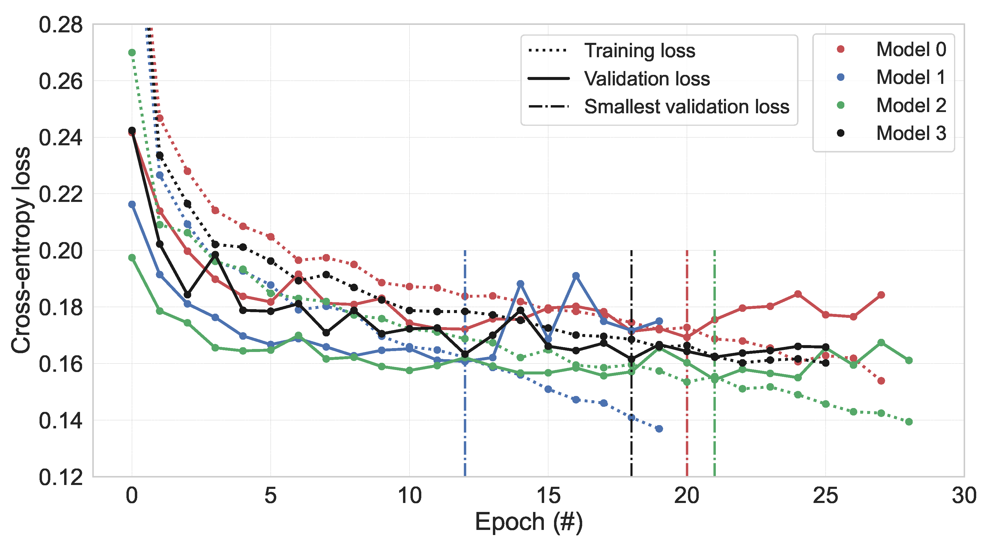
The per-epoch cross-entropy training and validation losses for the four models are depicted in Figure 4.

It can be seen that each model takes a different number of epochs to train. The model which had implemented Z-score normalization only showed to have very quickly diverging training vs. validation losses. On the other hand, the random Gaussian noise injection shows very good generalization capabilities as the trends in the training and validation losses are relatively closely related.

5.3. Sample Prediction Example

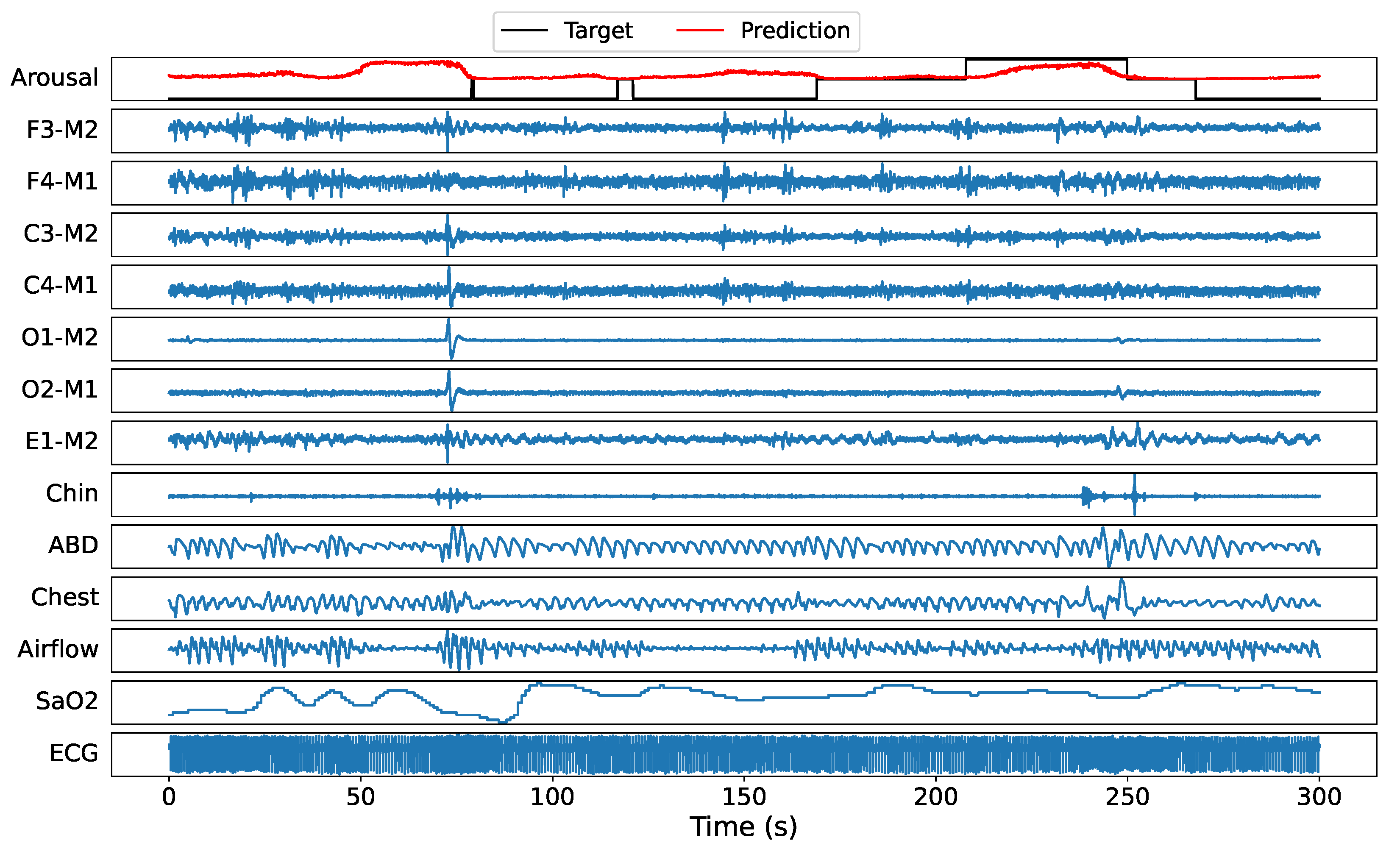
Before turning to the statistical results, a randomly selected recording (tr03-0078) from the test set is used to illustrate the DeepSleep 2.0 (model 2) arousal predictions. A 300 s window example of all 13 PSG channels with target labels and predicted sleep arousals at 5 ms resolution is illustrated in Figure 5. It can be seen that the model predicts a higher score at time windows where actual arousal happens. Note that ’-1’ represents nonscored regions, hence the model is allowed to output any score in these regions, see Section 4.4 for more details. On the other hand, nonarousal regions are accurately represented by low probability values.

5.4. Overall Results

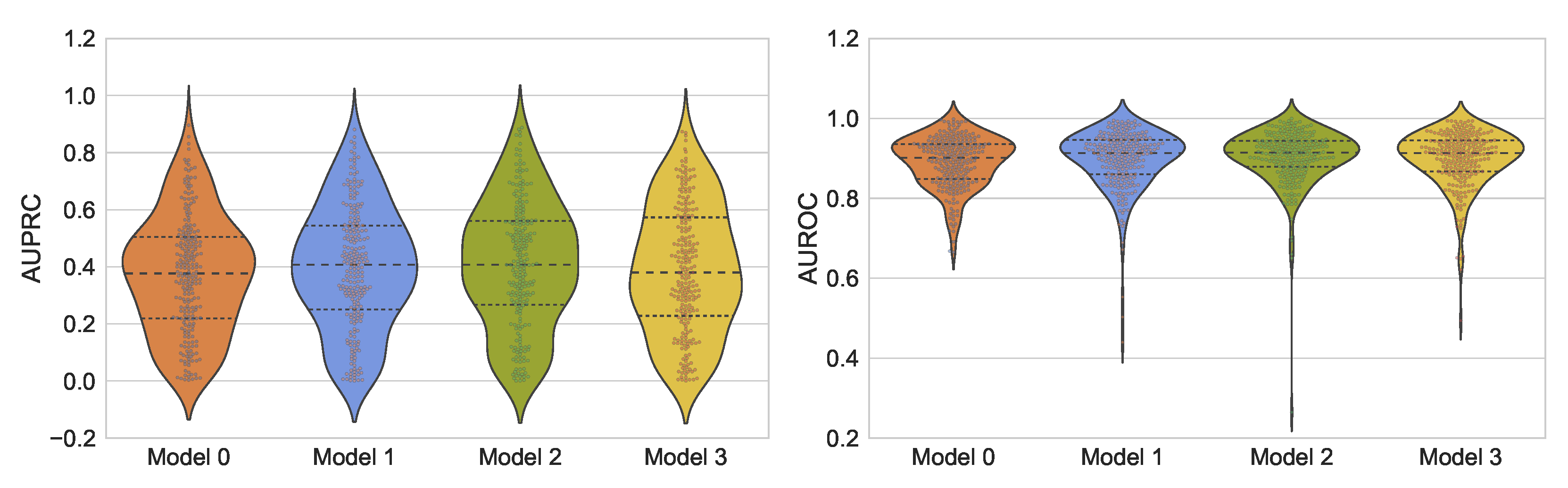
The models achieving the smallest validation loss were evaluated on the 25% of the held-out test data. The obtained results in terms of sample AUPRC and sample AUROC scores are reported in Figure 6.

The gross AUPRC, gross AUROC, and the BCE loss are summarized in

Table 4. Gross AUPRC, gross AUROC, and BCE for the test set.

Evaluation Metric	Model 0	Model 1	Model 2	Model 3
AUPRC	0.387872	0.443655	0.450434	0.407079
AUROC	0.878906	0.894429	0.901215	0.895116
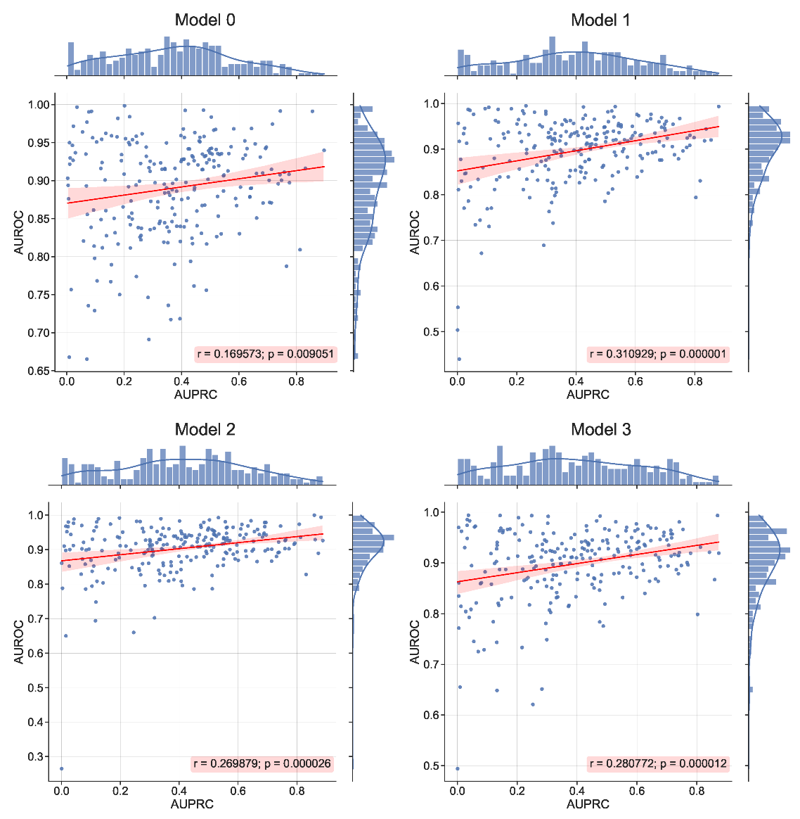
BCE	0.177034	0.166627	0.164296	0.170024

. Furthermore, the obtained sample AUPRC and AUROC scores were analyzed for potential correlation patterns, see Figure 7.

6. Discussion

The obtained results suggest that both the Z-score normalization and the similar PSG channel swapping are effective preprocessing and data augmentation techniques. The “bold” data augmentation strategy in terms of Gaussian noise injection did not lead to significant performance improvements, although it outperformed the baseline Model 0. The obtained results for Model 2 imply a possible second place in the 2018 PhysioNet challenge [3]. Compared to other architectures, DeepSleep 2.0 offers a much lighter model architecture while maintaining close to state-of-the-art performance. For all four model variants, with a significant p-value, a relatively weak but positive correlation is observed between the reported sample AUROC and AUPRC scores, suggesting a reliable overall assessment in terms of AUROC and AUPRC.

In the course of the network development and implementation, several aspects, not mentioned earlier, were considered. For instance, the model without Z-score normalization posed a significant challenge to the Adam optimizer, resulting in NaN values in the batch-normalization phase of the network. Gradient clipping did not solve this issue; however, committing to smaller learning rates did. Similarly, several experiments were performed on a smaller dataset. Various activation functions (ELU, SELU, GELU, ReLu), optimizers, data augmentation techniques, and weight initialization strategies were investigated.

In more generic terms, the author acknowledges that there are other open problems in automatic sleep arousal detection from multichannel PSG recordings. One of them is the absence of continuous labels. According to the AASM scoring manual, human experts provide only binary, i.e., “sleep” or “arousal”, labels while deep neural networks have the capability of predicting continuous labels (probability of arousal). Similarly, the quality of labels is often not perfect due to human errors. Therefore, a question arises how to obtain or fabricate quality labels that can be directly used to train a network that performs continuous predictions. On the other hand, there is still room to improve the prediction accuracy and/or efficiency. Finally, the determination of an optimal subset of physiological signals necessary to achieve a prescribed sleep arousal detection performance for a fixed architecture remains largely a heuristic task. Hopefully, this and similar studies will promote the potential of deep-learning-based techniques for automated nonapnea sleep arousal segmentation, offering close-to-human performance and leading to more efficient and cost-saving diagnosis procedures. Consequently, more patients may have access to timely and targeted treatments of arousal-related sleep disorders.

7. Conclusions

This work demonstrated that a more compact architecture of the state-of-the-art DeepSleep is able to perform automatic sleep arousal segmentation with a less-complex architecture, fewer parameters, and achieving close to similar AUPRC and AUROC scores on the held-out test data considered in this work. It should be noted that the original DeepSleep model achieved the high AUPRC score of 0.550 and AUROC score of 0.927 reported in PhysioNet challenge for its 1/8 + 1/2 + full ensemble model variant, almost tripling its base inference complexity. The computational complexity of the proposed DeepSleep 2.0 architecture is significantly smaller than its predecessor. The total number of trainable parameters in DeepSleep 2.0 is 740,551 and its depth is only 5, while DeepSleep relies on a depth of 11. To realize a very low-computational and low-memory practical application, the input signal should be downscaled and the layer input/output dimensions adequately modified. Future work is expected to consist of various attempts to further improve the model performance, reduce its complexity, and try new data-centric approaches. Ensemble models and the incorporation of categorical features are a few examples of other avenues to take.