Client Selection in Federated Learning under Imperfections in Environment

Abstract

Federated learning promises an elegant solution for learning global models across distributed and privacy-protected datasets. However, challenges related to skewed data distribution, limited computational and communication resources, data poisoning, and free riding clients affect the performance of federated learning. Selection of the best clients for each round of learning is critical in alleviating these problems. We propose a novel sampling method named the irrelevance sampling technique. Our method is founded on defining a novel irrelevance score that incorporates the client characteristics in a single floating value, which can elegantly classify the client into three numerical sign defined pools for easy sampling. It is a computationally inexpensive, intuitive and privacy preserving sampling technique that selects a subset of clients based on quality and quantity of data on edge devices. It achieves 50–80% faster convergence even in highly skewed data distribution in the presence of free riders based on lack of data and severe class imbalance under both Independent and Identically Distributed (IID) and Non-IID conditions. It shows good performance on practical application datasets.

1. Introduction

In this era of artificial intelligence, machine learning algorithms are data hungry. Models require large volumes of data to generalize well to practical use cases [1]. In reality, data are decentralized over different devices under privacy restrictions [2]. Federated learning provides an elegant solution. It involves a global cloud model that collaborates with a federation of devices called clients that carry private local data and execute a subroutine of local refinements in each round of communication [3]. This preserves the privacy as well as decentralizes learning to make better use of local resources while contributing to a global cloud model.

There are multiple challenges in federated learning [4]. Data skewness is the most popular among them. In ideal cases, Independent and Identically Distributed (IID) data are desired, both in terms of features as well as classes. However, in real scenarios, non-IID data varying from moderate to strongly skewed distribution is inevitable [5,6]. The global class imbalance problem may prevail and adversely affect the performance of the global model [7]. Further, communication challenges contribute towards cost and complexity of learning. The clients have limited and unequal computational power, thereby limiting the potential of learning at a local scale and affecting the global model as well [8]. There is another challenge related to client behaviors, known as free riders. Free riders [9] use the global model but do not contribute to learning. Free riders not only hog the limited communication resources, but also deteriorate the performance by contributing fake or low volume data in order to access the global model.

State-of-the-art federated learning algorithms include synchronous Federated Averaging (FedAvg) [10], Federated Stochastic Variance Reduced Gradient (FSVRG) [11] using Stochastic Variance Reduced Gradient (SVRG) [12] and asynchronous Cooperative Learning (CO-OP) [13]. These perform well on most of the real-world datasets with FedAvg outperforming FSVRG and CO-OP [14]. Federated multi-task learning has been shown as an effective paradigm to handle real-world datasets. An effective multi-task learning algorithm is VIRTUAL, which considers the federated system of server and clients as a star-shaped Bayesian network, and learning is performed using variational inference with unbiased Monte Carlo estimation [15]. However, the performance of all these methods depends on the important step of client selection in each round of refinement. The problem of client selection in an effective manner is the focus of this paper.

In an ideal situation, the best suited clients should be allowed to interact with the global model such that performance deterioration due to data skewness, class imbalance, and free riders can be minimized. The common approach is random client sampling. Some other approaches have also been reported. The asynchronous COOP protocol relies on age filters to allow merging of selected clients only. The age filters perform a prior verification of whether the client is active or old and if it lies in the specified age bandwidth. While age is a useful metric, it does not account for the data quality and quantity of the client. The resource-based client selection protocol FedCS [16] actively manages the clients based on resource constraints and accelerates the performance of the global model with the aim of aggregating as many devices as possible within a pre-defined time window. In [17], an optimal client selection strategy to update the master node is adopted based on a formula for optimal client participation. Another approach in [18] is based on adapting an online stochastic mirror descent algorithm to minimize the variance of gradient estimation. The approach mentioned in [19] takes into account overheads incurred on each device when designing incentive mechanisms to encourage devices with higher-quality data to participate in the learning process. However, tackling the free riders remains an open problem.

Some free riders’ attack and defense strategies were discussed in [9]. Free riders were identified by constructing local gradients without any training on data. Gradients based on random weights and delta weights are described as a possible free rider attack strategy. Such attacks can be prevented using a deep autoencoding Gaussian mixture mode (DAGMM) and standard deviation DAGMM [20]. More complex free riders disguising schemes based on additive stochastic perturbations and time varying noise models are discussed in [21]. In either of these schemes, a free rider client with zero data points can participate by reporting fake gradients. Another problem is that there may be free riding clients with small data volumes but with sufficiently large gradients to adversely affect the global model. In order to counter this situation, free riders can be identified as the clients with relatively small data volumes such that they do not have anything substantial to contribute to the learning of the global model. This allows weighing down such clients irrespective of other aspects. Active federate learning (AFL) [22] does use a client sampling method that takes into account the data volume of clients, and therefore, it has some cushion for free riders. Furthermore, its client sampling method includes consideration of class imbalance in binary classification problems. In our own experience, AFL can support multi-class, but the performance is bad when the free rider situation is present, and non-IID conditions make it worse. It also cannot handle the issue of severe lack of data. In other words, there is an unfulfilled need for client sampling schemes that handle the real-world situation where the issues of free riders, multi-class imbalance, non-IID, and extreme data skew coexist. To solve these issues and design a versatile and robust sampling approach, we propose:

• A novel single floating point score, namely the irrelevance score, which is sufficient for scoring the clients based on data volume, local class imbalance, as well as IID and non-IID conditions. The score is further scalable in the future to include other considerations.
• A novel client sampling method, namely irrelevance sampling, which uses the irrelevance score in an effective manner in order to enable a selection of optimal subset of clients for subsequent learning even in challenging imbalanced and free-rider ridden environments.

We validate the utility of our irrelevance score and the performance of our client sampling approach extensively using various numerical experiments, which include non-IID conditions, highly imbalanced federated environments, and moderate-to-severe free-riders’ repleted environments. We show the integrability and robust performance of the proposed sampling approach in diverse learning schemes and illustrate the superior performance over state-of-the-art sampling methods across three well-established simulated datasets and two real-world practical application datasets.

2. Proposed Approach: Irrelevance Sampling

We first present the novel irrelevance score, which is the foundation of our sampling method. The proposed novel scoring method performs well as compared to AFL and random sampling methods in our experiments under coexistence of free riders (clients with very less data samples), severe class imbalance and highly skewed distribution of samples. We analyze the mathematical bounds and design insights of the irrelevance score. Further, we present our sampling algorithm along with insights and complexity analysis of the algorithm and privacy preservation of our approach.

2.1. The Irrelevance Score $\mathsf{{\rm Y}}$

2.1.1. Definition

A single floating point measure is often a preferred, communication inexpensive, manner of scoring the clients towards developing a client sampling strategy. The design of such a score should account for class imbalance, non-IID data, as well as free riding characteristics. Our novel irrelevance score $\mathsf{{\rm Y}}$ for an mth client is therefore defined as a product of three components; namely, irrelevance score associated with free riders (${\mathsf{{\rm Y}}}_{\mathrm{FR}}$), irrelevance score associated with class imbalance (${\mathsf{{\rm Y}}}_{\mathrm{CI}}$), and irrelevance score associated with non-IID data (${\mathsf{{\rm Y}}}_{\mathrm{NIID}}$), as described below:

$$\mathsf{{\rm Y}}={\mathsf{{\rm Y}}}_{\mathrm{FR}}{\mathsf{{\rm Y}}}_{\mathrm{CI}}{\mathsf{{\rm Y}}}_{\mathrm{NIID}}$$

(1)

Here, we define the irrelevance score for free riders as:

$${\mathsf{{\rm Y}}}_{\mathrm{FR}}=\frac{1}{log\left(V_m\right)}$$

(2)

where $V_m$ is the data volume at the client. This is based on the consideration that free riders are clients that contribute a small data volume to the global model for learning. It is well-known that datasets with a large number of records are good for training and statistical analysis, as the statistical soundness of results increases with the number of observations. Therefore, Equation (2) non-linearly weighs the clients with small data volume as highly irrelevant.

The irrelevance score for class imbalance is defined as:

$${\mathsf{{\rm Y}}}_{\mathrm{CI}}=\sum _{n=1}^{N_o}{C}_{n}log\left(\frac{V_m}{V_{c_n}}\right)$$

(3)

where $V_{c_n}$ is the data volume for the nth class available at the client, $V_m$ is the total data volume at the client given by $V_m={\sum }_{n=1}^{N_c}{V}_{c_n}$, $N_c$ is the number of categories available on the client, and $N_o$ is the total number of categories in the problem. Lastly, $C_n$ refers to a boolean value indicating whether the nth category is available on this client or not. Here, we explain the working principle of this irrelevance score for the class imbalance. A class-imbalanced dataset is a collection of data points where observations of classes are not equal while a balanced dataset is a collection of equal observations of classes. A statistical classifier has a natural tendency to pick up the patterns in the most popular classes and ignore the least popular ones, thereby contributing a bias to the global model as well. The logarithm of $V_m/V_{c_n}$ for each class label accounts for local class imbalance at the client side. Further, the use of $C_n$ helps in identifying the relevance of the local dataset in the global context.

For defining the irrelevance component for the non-IID data, we introduce a function $f\left(x\right)$ below.

$$f\left(x\right)=\{\begin{array}{cc}\hfill 1& \mathrm{if}x>0\hfill \\ \hfill -1& \mathrm{otherwise}\hfill \end{array}$$

(4)

and define the irrelevance score for non-IID data as follows:

$${\mathsf{{\rm Y}}}_{\mathrm{NIID}}=N_c^{-1.75}f\left(x\right)$$

(5)

where $x=N_c-(N_o-1)/2$. The definition of x and $f\left(x\right)$ allow us to identify the clients that represent at least half the number of classes in the global model. We have included a modulating factor $N_c^{-1.75}$ in this term in order to make a good separation between good clients and bad clients. We need to keep the scores low for those clients that have a large number of categories in order to be as close as possible to the ideal IID situation in terms of categories. The choice of 1.75 here is empirical based on our observation that it works well for separating the scores well by a large difference.

2.1.2. Bounds of Irrelevance Score

The irrelevance score is a multivariate mathematical function. Here, we show that this mathematical function is bounded under all circumstances. We know that the number of classes is a natural number so $N_c\ge 1$. We divide our analysis into two cases: Case A ($N_c\ge 2$) and Case B ($N_c=1$).

Case A ($N_c\ge 2$): Since $V_{c_n}\in \mathbb{N}$, hence $V_{c_n}\ge 1$ and the following conditions are true: $V_m/V_{c_n}\in [1, V_m]$, and therefore, $log(V_m/V_{c_n})\in [0, log\left(V_m\right)]$. Consequently, using Equation (3), the following also hold:

$$0<{\mathsf{{\rm Y}}}_{\mathrm{CI}}\le \sum _{n=1}^{N_o}{C}_{n}log\left(V_m\right)\le N_{c}log\left(V_m\right)$$

(6)

Further, due to the nature of the function $f\left(x\right)$ in Equations (4) and (5), the bounds on ${\mathsf{{\rm Y}}}_{\mathrm{NIID}}$ are given as

$${\mathsf{{\rm Y}}}_{\mathrm{NIID}}\in \left[-N_c^{-1.75}, 0)\cup (0, N_c^{-1.75}\right]$$

(7)

It is interesting to note that the range of ${\mathsf{{\rm Y}}}_{\mathrm{NIID}}$ comprises two mutually exclusive sets, one with strictly negative values and the other with strictly positive values. Using Equation (4), their common non-inclusive boundary is encountered at $x=0$, i.e., when $N_o=2N_c+1$. In order to be as close as possible to IID situations, the clients with number of local classes more than or equal to half the number of global classes are automatically assigned positive values indicating a more relevant client in terms of number categories. The choice of 50% (half the number of classes) is empirically chosen based on our observations. Lastly, using Equations (1), (2), (6) and (7), the bounds on the irrelevance score $\mathsf{{\rm Y}}$ are determined as:

$$\mathsf{{\rm Y}}\in \left[-N_c^{-0.75}, 0)\cup (0, N_c^{-0.75}\right]$$

(8)

Given the condition $N_c\ge 2$, the bounds are specified by $N_c=2$ and therefore $\mathsf{{\rm Y}}\in \left[-2^{-0.75}, 0)\cup (0, 2^{-0.75}\right]$.

Case B ($N_c=1$): $N_c=1$ implies clients with single class, which results in $V_{c_n}=V_m$. Hence, according to Equation (3), ${\mathsf{{\rm Y}}}_{\mathrm{CI}}=0$. Consequently, using Equation (1), $\mathsf{{\rm Y}}=0$.

Taking the union of results from the cases A and B, we conclude that $\mathsf{{\rm Y}}\in \left[-2^{-0.75}, 2^{-0.75}\right]$.

2.1.3. Design Insights

We summarize the inherent characteristics of the irrelevance score here. First, the irrelevance score is zero for the clients that represent data of only one class in their local dataset. This is a consequence of ${\mathsf{{\rm Y}}}_{\mathrm{CI}}$ defined in Equation (3). Second, as a consequence of ${\mathsf{{\rm Y}}}_{\mathrm{NIID}}$ defined in Equation (5), the irrelevance score has positive values for the clients that represent more than half the number of classes in the global model. Third, the clients with less data volume are assigned a higher irrelevance score as a consequence of ${\mathsf{{\rm Y}}}_{\mathrm{FR}}$ defined in Equation (2). Lastly, the class imbalance within the local dataset of the client also results in high irrelevance score due to ${\mathsf{{\rm Y}}}_{\mathrm{CI}}$. Hence, we consider good clients that have irrelevance score closer to zero except for the case of $\mathsf{{\rm Y}}=0$.

We note that clients with more than half the number of categories ($\mathsf{{\rm Y}}>0$) are closer to the ideal IID situation and therefore more preferable over other clients ($\mathsf{{\rm Y}}\le 0$). However, this may not hold true for some highly skewed distributions where few categories are present only with clients that have a much lower number of categories ($\mathsf{{\rm Y}}<0$) or have only a single category ($\mathsf{{\rm Y}}=0$). We note that in real-world scenarios, it is possible that certain classes are very rare and present only on single category clients. Hence, it is not a good decision to ignore clients with a single category. We use the irrelevance score intuitively to handle such problems, as described in Section 2.2. We argue that there are indeed other candidate functions of the three components. However, our design is motivated by two main factors. First, a client that is a poor candidate in any of the three aspects is a poor client irrespective of its suitability in terms of the other aspects. A multiplicative function of their unsuitability (or irrelevance) is therefore a simple and effective solution. Second, such a simple multiplicative design is easily scalable to include other aspects in the future as the field of federated learning evolves and more concerns are identified in the matter of client selection.

2.1.4. Insights of Varying Individual Components

We study the effect of various parts of the equation by using graphical and mathematical representations.

Figure 1 shows the variation of the free rider component of Irrelevance score (${\mathsf{{\rm Y}}}_{\mathrm{FR}}$) with respect to total data volume ($V_n$). The value of ${\mathsf{{\rm Y}}}_{\mathrm{FR}}$ decreases with increasing data volume making clients with a higher data samples more relevant.

Figure 2 shows the variation of the Non-IID component of Irrelevance score (${\mathsf{{\rm Y}}}_{\mathrm{NIID}}$) with respect to the number of unique categories on a client for a problem with 20 global classes. Clients falling in the zero pool ($S_o$ have ${\mathsf{{\rm Y}}}_{\mathrm{NIID}}$ = 0 at $N_c$ = 0. Clients with less than half the number of categories ($N_c<10$) have negative scores (negative pool $S_{-}$) while clients with more than half the number of categories ($N_c\ge 10$) have positive scores (positive pool $S_{+}$). Furthermore, as the number of categories increases, the magnitude of ${\mathsf{{\rm Y}}}_{\mathrm{NIID}}$ approaches zero, making clients with a higher amount of categories more relevant.

Ideally, clients with higher degree of imbalance are not relevant (higher $\mathsf{{\rm Y}}$). Here, the analysis of $\mathsf{{\rm Y}}$ under highest possible degree of imbalance is shown. Using Equation (6), we can see that the maximum value of ${\mathsf{{\rm Y}}}_{\mathrm{CL}}$ is achieved when ${\mathsf{{\rm Y}}}_{\mathrm{CL}}=N_{c}log(V_n$).

Using Equations (1), (2), (5) and (6):

$$\mathsf{{\rm Y}}=N_c^{-0.75}f\left(x\right)$$

(9)

Figure 3 shows the variation of Equation (9). Under maximum imbalance, the client has a higher magnitude of $\mathsf{{\rm Y}}$, as shown in Figure 3 in comparison to Figure 2. This shows if the client has a high degree of imbalance in that the class imbalance component outweighs the benefit of a high number of classes, resulting in an overall high $\mathsf{{\rm Y}}$ score.

2.2. Sampling Algorithm

We have seen how the irrelevance score wraps up the information of a client based on data volume, imbalance and number of classes into a single floating point value. In this section, we present a sampling algorithm that leverages the irrelevance score of clients to define the probability distribution of the selection of clients in subsequent rounds of training.

In federated learning, M clients are associated with M datasets $D_1,\cdots ,D_M$, where $D_m$ denotes the dataset of the mth client. $D_m$ is generated by a client-dependent probability distribution function and is accessible by the respective client only. The volume of each dataset at a particular client depends on the type of environment in which the client is present, as described in Section 3.1.2. In each round of training, we sample a fixed number of K clients from a pool of M clients. Hence, the aggregation of weights in training is highly dependent on which clients were sampled in each round. This selection of clients is performed by the server model in each round. In order to simulate the real-world characteristics we assume that the data keeps on changing at the client end.

In each round, we collect the scores ${\mathsf{{\rm Y}}}_1,\dots ,{\mathsf{{\rm Y}}}_M$ from all clients. Utilizing the characteristics of the irrelevance score $\mathsf{{\rm Y}}$ discussed in the previous section, we make three pools of clients named positive, negative and zero pool. They are denoted by $S_{+}$, $S_{-}$ and $S_o$ and correspond to the clients with positive, negative, and zero values of $\mathsf{{\rm Y}}$, respectively. A tolerance parameter ($\varphi$ = 3) is used to map the clients with the same score up to $\varphi$ decimal places in each pool separately. Clients with same scores are randomly shuffled in each pool separately, which prevents biased training on any client. Based on the scores, clients are sorted in ascending order of their magnitudes in each pool. We select a fraction of clients from the top of each pool based on three parameters. In essence, we select the clients with scores closest to zero, as shown in Figure 4. These parameters are $\alpha$ for positive pool, $\beta$ for negative pool and $\gamma$ for zero pool, such that $\alpha +\beta +\gamma =1$ and $\alpha \ge \beta \ge \gamma$. Let $C_{\alpha }$, $C_{\beta }$ and $C_{\gamma }$ denote the subsets of $S_{+}$, $S_{-}$ and $S_o$, which contain the selected clients for the next round, respectively. They contain the top $\alpha K$, $\beta K$ and $\gamma K$ clients from the respective pools. Proper selection of $\alpha , \beta , \gamma$ ensures smoother and faster convergence, as we demonstrate later in our experiments.

For demonstration purposes, we consider $\alpha =\beta =\gamma$ in Figure 5 with a total of five classes in the classification problem colored in Green, Red, Orange, Yellow, and Violet. Client C1 demonstrates a perfectly balanced client with four classes, C2 demonstrates a free rider with four classes, C3 demonstrates a highly imbalanced client with two classes, C4 is a single class client with a rare class, which is not present on any other client, C5 depict four-class highly imbalanced case and C6 depict a two-class nearly balanced case. According to our method, C1, C2 and C5 belong to $S_{+}$, C3, C5 belongs to $S_{-}$ and C4 belongs to $S_o$ pool. For sampling the best three clients with $\alpha =\beta =\gamma$, our method will select C1, C6 and C4 and reject the free rider case of C2 and imbalanced cases of C6 and C3.

2.2.1. Design Insights of $S_{+}$, $S_{-}$ and $S_o$ Pools with $\mathsf{{\rm Y}}$

Assigning ${\mathsf{{\rm Y}}}_{\mathrm{CL}}=1$ in Equation (1) results in the dependence of $\mathsf{{\rm Y}}$ only on ${\mathsf{{\rm Y}}}_{\mathrm{FR}}$ and ${\mathsf{{\rm Y}}}_{\mathrm{NIID}}$ as shown below.

$$\mathsf{{\rm Y}}={\mathsf{{\rm Y}}}_{\mathrm{FR}}{\mathsf{{\rm Y}}}_{\mathrm{NIID}}$$

(10)

Using Equations (2), (5) and (10)

$$\mathsf{{\rm Y}}=\frac{N_c^{-1.75}f\left(x\right)}{log\left(V_m\right)}$$

(11)

Figure 6 shows the variation of $\mathsf{{\rm Y}}$ under this condition. Curve below the x-axis corresponds to clients in the negative pool ($S_{-}$), while the curve above the x-axis corresponds to positive pool ($S_{+}$). In either case, the score approaches zero as the data volume and number of categories are increased, resulting in a higher relevance of clients with high data volume and number of categories.

2.2.2. Insights of Varying $\alpha , \beta , \gamma$

The variation of three parameters of the irrelevance score is shown in Figure 7. We note that the performance improves drastically with the increasing $\alpha$ parameter while the $\beta$ parameter shows a moderate increase in performance. The $\gamma$ parameter shows an inverse relation with performance. The following relations hold while considering variations of a particular parameter.

Variation of parameter $\alpha$.

$$\begin{array}{c}\alpha =x\end{array}$$

(12)

$$\begin{array}{c}\beta =\gamma =(1-x)/2\end{array}$$

(13)

Variation of parameter $\beta$.

$$\begin{array}{c}\beta =x\end{array}$$

(14)

$$\begin{array}{c}\alpha =\gamma =(1-x)/2\end{array}$$

(15)

Variation of parameter $\gamma$.

$$\begin{array}{c}\gamma =x\end{array}$$

(16)

$$\begin{array}{c}\alpha =\beta =(1-x)/2\end{array}$$

(17)

Considering equivalence of any two parameters, we obtain the following condition.

$$\begin{array}{c}x=(1-x)/2\end{array}$$

(18)

$$\begin{array}{c}x=1/3\approx 0.33\end{array}$$

(19)

This condition is depicted by the approximate intersection of the three curves in Figure 7.

2.3. Complexity Analysis

The algorithm is presented in Algorithm 1. Here, we analyze the time and space complexity of the sampling algorithm in the worst case scenarios. In step (10), we sort the clients into the three pools separately using the Timsort method [23]. This sorting method is stable and beats every other sorting algorithm in time. It has a time complexity of $\mathsf{\Omega }\left(M\right)$ in the best case, $\theta (Mlog(M\left)\right)$ on an average and $\mathcal{O}(Mlog(M\left)\right)$ in the worst case. Apart from this, the space complexity of Timsort is $\mathcal{O}\left(M\right)$. We store the scores for performing operations on them, hence the space complexity is $\mathcal{O}\left(M\right)$.

Algorithm 1: Sampling Algorithm.

2.4. Differential Privacy

Encapsulating information of client in a single floating point value preserves the privacy of qualitative aspects of local data. Only a vague idea regarding relative goodness of clients is revealed in terms of data volume and imbalance. The score resulting from the product of the three components in (1) automatically hides the information regarding whether the client is a free rider, imbalanced in terms of data or a combination of these. The calculation of irrelevance score can be performed via a trusted method or application that denies the access of the server and clients in the process of score calculation. Hence, the authenticity of score is preserved by all means. However, both AFL and the proposed sampling methods face limitations under the scenario when scores returned are not trustable.

3. Experimental Evaluation

In this section, we report extensive performance evaluation of our client sampling method for both IID and non-IID conditions for 5 datasets and also compare this with the contemporary state-of-the-art sampling methods.

3.1. Experimental Settings

In our experimental evaluation, we not only consider 3 simulated and 2 practical datasets (see

Table 1. Description of datasets used in the experiments. The numbers in parentheses in the first column indicate the number of classes. The entries in the 2nd and 3rd columns represent the total number of samples, mean number of samples per class ± standard deviation of number of samples per class.

Dataset	Training Samples	Validation Samples
MNIST (10)	60,000, 6000 ± 322	10,000, 1000 ± 59
KMNIST (10)	60,000, 6000 ± 0	10,000, 1000 ± 0
FEMNIST (47)	112,800, 2400 ± 0	18,800, 400 ± 0
VSN (2)	41,057, 20,528 ± 1931	7246, 3623 ± 340
HAR (6)	8754, 1459 ± 164	1545, 257 ± 26
CTG (21)	1913, 293 ± 241	213, 30 ± 25

), we also simulate different challenging environments and include the consideration of learning algorithms as well (see

Table 2. Details of experimental variations considered for both IID and non-IID situations.

Sampling Approaches	Learning Approaches
R: Random sampling	FedAvg: Federated averaging
A: AFL sampling	FSVRG: Naive federated SVRG
I: Irrelevance sampling	COOP: Cooperative Learning
Simulated Environments
E1: highly balanced environment
E2: highly imbalanced environment
E3: moderately free-rider repleted environment
E4: general real-world user environment
E5: severe free-rider repleted environment
E6: extreme free-rider repleted environment

). All the datasets represent classification problems and the classification accuracy is used as a performance indicator.

3.1.1. Balanced and Imbalanced

We performed our experiments based on different federated environments under both balanced and imbalanced conditions. Here, balanced conditions mean that all of the classes of the classification problem being solved have equal amount of training and validation samples, while in the case of the imbalanced scenario, a certain number of classes have significantly less training and validation samples. More specifically, four, four, eighteen, one and two classes are imbalanced in the MNIST, KMNIST, FEMNIST, VSN and HAR datasets, respectively.

3.1.2. IID and Non-IID Conditions

IID stands for independent and identically distributed data, while Non-IID stands for non-independent and non-identically distributed data. The distribution of data among clients can be described in terms of feature distribution as well as class distribution. MNIST, KMNIST and EMNIST-47 describe the IID features across the data points while VSN strongly describes non-IID feature distribution. In the real-world, Non-IID data on clients both in terms of feature and class distribution is inevitable and hampers the performance of the global model. We simulate the label wise Non-IID distribution of the mentioned datasets in the experiments.

For IID conditions, all clients have all categories present in their local data, while in the Non-IID condition, a variable number of categories ranging from a single category to 70% of total categories are present on the clients. More specifically, an equal number of four types of clients with 70%, 50%, 30% and 10% classes in case of MNIST, KMNIST, FEMNIST and Cardiotocography(CTG) are simulated. In the case of the VSN dataset, clients equal number of one and two classes are simulated, and in the HAR dataset, clients with an equal number of two, three and four classes are simulated. Depending on the type of environments (E1-E6), the volume of datasets on each client also varies, as mentioned in

Table 3. Definition of datasets associated with each client under different environments.

Type	Nature	Training Data:Validation Data	Free Riders?
I	Balanced	400:60	No
II	Imbalanced	400:60	No
III	Balanced	100:20	No
IV	Imbalanced	100:20	No
V	Balanced	50:10	Yes
VI	Balanced	20:4	Yes

.

3.1.3. Federated Environments

In all of our experiments we use a federated system of 100 clients and sample 10 clients in each round of training unless stated otherwise. We create clients of six types and use different proportions of these types of clients to create different environments. The environments and types are presented in

Table 4. Definition of different federated environments.

	Type of Client
	I	II	III	IV	V	VI
E1	0.90	0.02	0.02	0.02	0.02	0.02
E2	0.02	0.90	0.02	0.02	0.02	0.02
E3	0.04	0.04	0.04	0.04	0.40	0.40
E4	0.17	0.17	0.17	0.17	0.16	0.16
E5	0.02	0.02	0.04	0.04	0.44	0.44
E6	0.01	0.01	0.01	0.01	0.48	0.48

. We note that Type V and VI demonstrate the behavior of a free rider in terms of lack of data and contributing significantly less towards the global model. E1 to E4 are used for generating results for individual datasets. Further, E5-E6 are used in ablation and convergence studies.

3.1.4. Architectures

In the experiments, multilayer perceptrons (MLP) are employed. In the case of MNIST and VSN datasets, two hidden dense flipout layers each of 100 units and an ReLU activation function with a final layer of 10 and 2 units, respectively, were used. In the case of KMNIST, FEMNIST and HAR datasets single hidden dense flipout layer of 512 units and ReLU activate function with final layer of 10, 47 and 6 units respectively were used. In the Cardiotocography dataset, 5 hidden layers of 21 units each are used with the final output layer of 10 units. In all cases, softmax activation is applied on the final layer.

3.1.5. Learning Parameters

The learning rate is kept at 0.003 for all cases. We perform 50 rounds of refinement in the global model and in each round of training, 10 clients are used to update the global model based on the sampling method with a single refinement per client. Some relevant details of the learning algorithms are presented here. We have used the naive Federated SVRG (FSVRG) as described in Algorithm 3 of [11]. The step size parameter h is set as 1.0. The CO-OP algorithm, as described in Algorithm 3.1 of [13], is used with age filter parameters a and b as 7 and 21, respectively.

3.1.6. Parameters of the Proposed Irrelevance Sampling Method

The parameters of the proposed algorithm are set as $\alpha =1.0$, $\beta =0.0$ and $\gamma =0.0$ for IID and $\alpha =0.5$, $\beta =0.3$ and $\gamma =0.2$ for non-IID settings unless stated otherwise.

3.2. Results for Individual Datasets

Results for MNIST dataset: It comprises gray scale images of handwritten single digits between 0 and 9, each of size $28\times 28$ pixels. The problem is to classify the image as belonging to the class of the digit [24]. The results for this dataset are presented in

Table 5. Classification accuracies for dataset MNIST.

	IID			Non-IID
	R	A	I	R	A	I
Learning method FedAvg
E1	0.95	0.95	0.96	0.85	0.91	0.91
E2	0.76	0.86	0.88	0.87	0.88	0.90
E3	0.88	0.66	0.91	0.84	0.72	0.88
E4	0.91	0.84	0.94	0.88	0.87	0.91
Learning method FSVRG
E1	0.94	0.94	0.95	0.88	0.88	0.89
E2	0.78	0.88	0.85	0.79	0.81	0.82
E3	0.88	0.83	0.91	0.75	0.53	0.80
E4	0.89	0.87	0.93	0.85	0.81	0.88
Learning method COOP
E1	0.90	0.83	0.90	0.79	0.72	0.87
E2	0.64	0.61	0.86	0.53	0.58	0.86
E3	0.61	0.17	0.90	0.54	0.14	0.86
E4	0.74	0.32	0.92	0.72	0.30	0.84
Learning method Virtual MTL
E1	0.84	0.86	0.87	0.66	0.73	0.75
E2	0.60	0.85	0.86	0.51	0.72	0.74
E3	0.32	0.77	0.86	0.28	0.39	0.71
E4	0.66	0.79	0.85	0.48	0.57	0.68

.

We notice that the environment E3 (free riders replete) is generally quite challenging for the AFL sampling, where it performs the poorest irrespective of the algorithm. The random sampling approach finds the imbalanced environment (E2) the most challenging for the IID condition and the free-riders repleted environment (E3) for the Non-IID conditions. Generally, both random and AFL sampling perform poorer when used in a COOP learning scheme while provide comparable performance for FedAvg and FSVRG learning schemes. We do notice the better performance of FedAvg than FSVRG for the Non-IID condition. As compared to random and AFL sampling, the proposed ’irrelevance’-based sampling approach performs the best among the three sampling methods irrespective of the environment, learning scheme, or the conditions (IID versus Non-IID). It provides the most balanced performance with small variations over different environments as well as different learning schemes. This demonstrates the robustness and versatility of the proposed sampling method. In the realistic environment E4, the clear edge of the proposed ‘irrelevance’-based sampling is evident, with at least 3% better classification accuracy than its contemporary in any environment, any condition, and with any learning scheme.

The poor performance of COOP and Virtual MTL for both AFL and random sampling is consistent through all the datasets. At the same time, there is no new insight about the proposed method specific for these schemes except that the performance of the proposed method is superior to that of the other sampling methods. Therefore, the results of these learning methods for the other datasets are not shown hereon.

3.2.1. Results for KMNIST Dataset

It is similar to MNIST, except that instead of digits, it represents hand-written Japanese characters of Hiragana [25]. The results for this dataset are presented in

Table 6. Classification accuracies for dataset KMNIST.

	IID			Non-IID
	R	A	I	R	A	I
Learning method FedAvg
E1	0.83	0.83	0.84	0.76	0.76	0.76
E2	0.50	0.65	0.66	0.66	0.66	0.67
E3	0.66	0.59	0.71	0.64	0.49	0.69
E4	0.73	0.61	0.79	0.61	0.66	0.71
Learning method FSVRG
E1	0.78	0.78	0.80	0.68	0.73	0.73
E2	0.49	0.64	0.66	0.61	0.63	0.67
E3	0.68	0.63	0.71	0.63	0.59	0.67
E4	0.70	0.67	0.77	0.65	0.64	0.70

. The KMNIST dataset is generally more challenging than the MNIST dataset, as witnessed in the poorer performance for any experiment. Nonetheless, the well-balanced environment (E1) is a relatively simpler environment and all sampling methods perform similarly to each other, although the proposed ‘irrelevance’ sampling method has a slight nominal edge. Further, for the imbalanced environment (E2), AFL sampling shows a clear advantage over random sampling, and the proposed sampling method provides a further better performance by a small margin. On the other hand, the advantage of the proposed ‘irrelevance’-based sampling is clearly evident in E3 and E4, where a performance superior by an average of 5% is observed over its contemporaries across all the cases.

3.2.2. Results for FEMNIST Dataset

The FEMNIST dataset is a federated version of the EMNIST dataset, containing both characters and digits. We used the balanced version with 10 single digit classes between 0 and 9 inclusive, 26 uppercase alphabets and 11 lowercase alphabets [26]. The results for this dataset are presented in

Table 7. Classification accuracies for dataset FEMNIST.

	IID			Non-IID
	R	A	I	R	A	I
Learning method FedAvg
E1	0.76	0.72	0.76	0.66	0.70	0.72
E2	0.41	0.56	0.54	0.58	0.59	0.59
E3	0.54	0.41	0.64	0.45	0.25	0.59
E4	0.64	0.50	0.72	0.58	0.48	0.66
Learning method FSVRG
E1	0.71	0.70	0.72	0.67	0.67	0.68
E2	0.41	0.50	0.46	0.59	0.60	0.62
E3	0.58	0.52	0.59	0.51	0.25	0.61
E4	0.60	0.58	0.68	0.59	0.52	0.65

. With a significantly larger number of classes, this is a significantly challenging dataset and an ideal simulated scenario to investigate the performance of federated learning. The effect is observed in the poorer performance of all the sampling methods for this dataset in comparison to MNIST and KMNIST datasets. Further, in general, the proposed irrelevance sampling method provides a significant advantage (7% to 14%) for the challenging E3 and E4 environments.

3.2.3. Results for the Vehicle Sensor Network (VSN) Dataset

A network of 23 different sensors (including seismic, acoustic and passive infra-red sensors) are placed around a road segment in order to classify vehicles driving past them [27]. The raw signal is processed into 50 acoustic and 50 seismic features. We consider every sensor as a client and perform binary classification of amphibious assault vehicles and dragon wagon vehicles. Being a real dataset for a practical application, it provides the challenges of real measurements. However, the problem involves only two classes and features a large dataset and, therefore, a relatively simpler situation than the three previous datasets. This dataset provides the performance of the proposed sampling method in the use cases where the number of categories is much less. The results for this dataset are presented in

Table 8. Classification accuracies for dataset VSN.

	IID			Non-IID
	R	A	I	R	A	I
Learning method FedAvg
E1	0.90	0.90	0.91	0.86	0.89	0.89
E2	0.69	0.80	0.85	0.66	0.77	0.85
E3	0.79	0.79	0.89	0.70	0.72	0.87
E4	0.80	0.81	0.91	0.78	0.79	0.89
Learning method FSVRG
E1	0.90	0.89	0.90	0.87	0.89	0.90
E2	0.56	0.84	0.83	0.53	0.81	0.82
E3	0.86	0.85	0.89	0.86	0.85	0.87
E4	0.86	0.84	0.89	0.86	0.82	0.89

. In general, the proposed irrelevance sampling either performs on par with or better than the other two sampling methods. Its clear advantage is evident for E2, E3 and E4 environments irrespective of the IID or Non-IID conditions or the learning scheme.

3.2.4. Results for Human Activity Recognition (HAR) Dataset

Recordings of 30 subjects performing daily activities are collected using smartphones with inertial sensors. The raw signal is divided into windows and processed into a 561-length vector [28]. Every individual corresponds to a different client, and we perform a classification of 6 different activities (walking, walking upstairs, walking downstairs, sitting, standing, laying). With 6 classes and relatively few samples per class (see Table 1), this dataset is quite challenging. The results are presented in

Table 9. Classification accuracies for dataset HAR.

	IID			Non-IID
	R	A	I	R	A	I
Learning method FedAvg
E1	0.93	0.95	0.92	0.73	0.81	0.82
E2	0.70	0.86	0.91	0.31	0.61	0.69
E3	0.90	0.87	0.94	0.75	0.74	0.93
E4	0.93	0.79	0.94	0.59	0.77	0.91
Learning method FSVRG
E1	0.90	0.85	0.91	0.87	0.87	0.87
E2	0.82	0.83	0.87	0.63	0.73	0.85
E3	0.86	0.81	0.89	0.74	0.64	0.80
E4	0.85	0.86	0.90	0.74	0.69	0.85

. The significant advantage of the proposed irrelevance sampling is evident in all the challenging environments (E2–E4), providing an improvement in classification accuracy of 3–18% for E2 and E3 and 1–14% for E4.

3.2.5. Results for Cardiotocography Dataset

The dataset consists of measurements of fetal heart rate (FHR) and uterine contraction (UC) features on cardiotocograms classified by expert obstetricians as described in [29,30]. Total 2126 fetal cardiotocograms (CTGs) were automatically processed and the respective diagnostic features measured with 21 training attributes. The CTGs were also classified by three expert obstetricians and a consensus classification label assigned to each of them. Classification was both with respect to a morphologic pattern (A, B, C. …) and to a fetal state (N, S, P). Therefore, the dataset can be used either for 10-class or 3-class experiments. This dataset has few samples per class and being a real-world problem in the medical field makes it very suitable for utilizing the proposed method under federated settings.

Table 10. Classification accuracies for dataset cardiotocography.

	IID			Non-IID
	R	A	I	R	A	I
Learning method FedAvg
E1	0.70	0.69	0.72	0.61	0.59	0.61
E2	0.32	0.55	0.65	0.51	0.52	0.55
E3	0.56	0.57	0.68	0.51	0.47	0.53
E4	0.48	0.52	0.69	0.58	0.55	0.60
E5	0.54	0.49	0.56	0.46	0.45	0.51
E6	0.51	0.46	0.54	0.44	0.41	0.49

shows the classification accuracies of using various sampling methods on this dataset using 10 morphological pattern categories. There is a significant advantage of using the proposed irrelevance sampling method under all challenging situations (E1–E6). The irrelevance sampling method outperforms other sampling methods by 2–10%.

3.3. Ablation Study

We perform an ablation study to validate the effectiveness of the proposed algorithm. First, we describe the affect of variation of the parameters $\alpha ,\beta$ and $\gamma$ on validation accuracy of the global model. Second, we describe the effectiveness of the proposed algorithm under moderate to severe free rider density through environments E5 and E6, respectively.

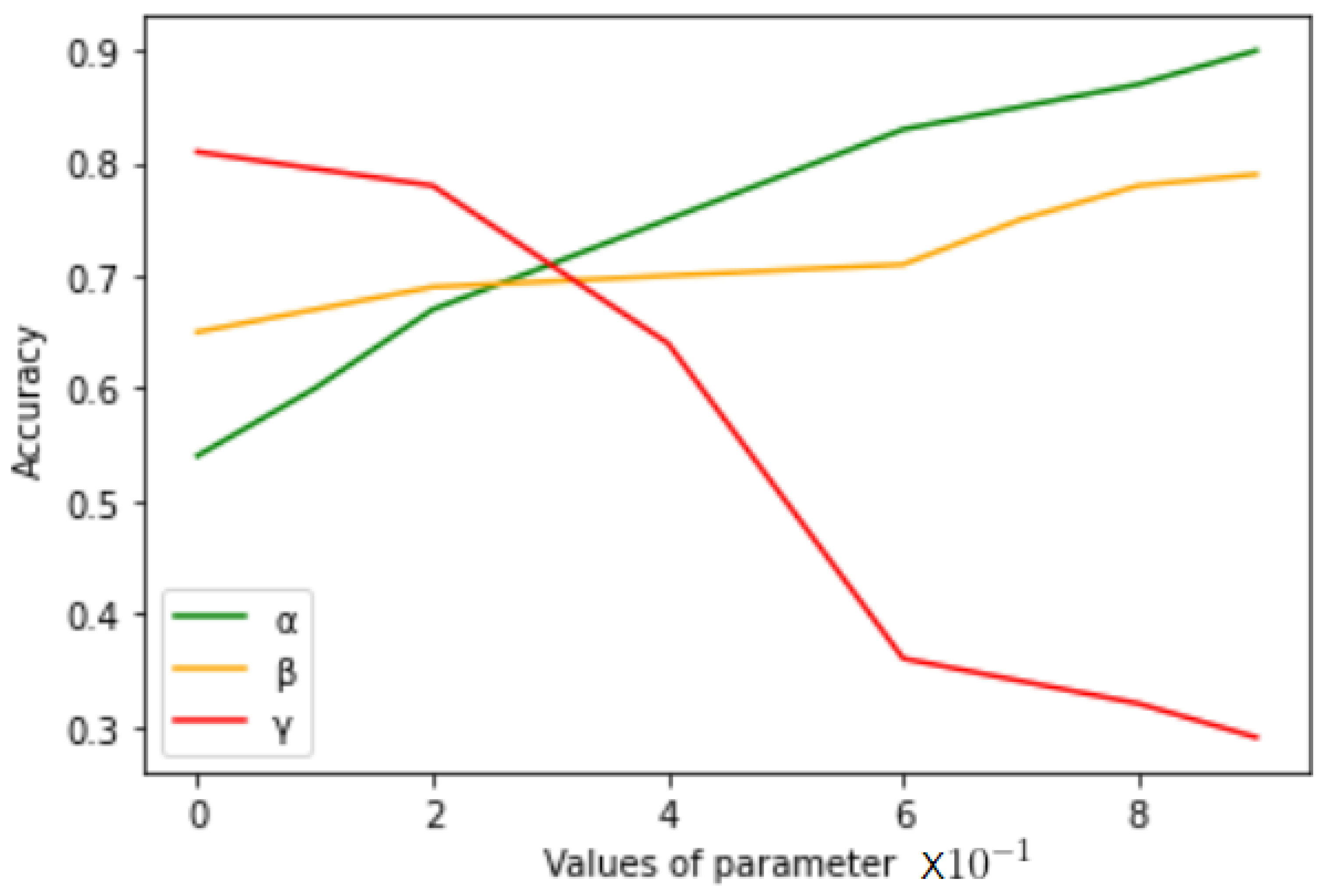
3.3.1. Variation of Parameters $\alpha , \beta , \gamma$

As described in Section 3.1, the parameters $\alpha , \beta$ and $\gamma$ control the distribution of selected clients. In

Table 11. Effect of varying $\alpha$, $\beta$ and $\gamma$ using Non-IID MNIST under FedAvg.

x	0.0	0.2	0.4	0.6	0.8
$\alpha =x, \beta =\gamma =\frac{1-x}{2}$	0.54	0.67	0.75	0.83	0.87
$\beta =x, \alpha =\gamma =\frac{1-x}{2}$	0.65	0.69	0.70	0.71	0.78
$\gamma =x, \alpha =\beta =\frac{1-x}{2}$	0.81	0.78	0.64	0.36	0.32

, we study the effect of various choices of the parameters. We clearly observe that as $\alpha$ is increased, the accuracy also improves rapidly. The variation of $\beta$ shows a moderate increase, while the variation of $\gamma$ is inversely related to accuracy.

3.3.2. Free Rider Density

The performance of the proposed sampling algorithm is compared with AFL and random sampling methods under severe (E₅) and extreme (E₆) conditions of free riders. From

Table 12. Accuracy comparison under severe to extremely severe free rider density environments. FedAvg learning algorithm and Non-IID conditions are used.

Dataset	E5			E6
	R	A	I	R	A	I
MNIST	0.77	0.65	0.88	0.65	0.55	0.87
KMNIST	0.51	0.46	0.65	0.46	0.43	0.61
FEMNIST	0.41	0.24	0.53	0.38	0.20	0.53
VSN	0.74	0.81	0.86	0.72	0.80	0.84
HAR	0.61	0.69	0.89	0.57	0.68	0.80

, it is evident that as the density of the free rider increases, there is a deterioration in the performance of all sampling methods. However, the proposed sampling method maintains the best performance in all cases.

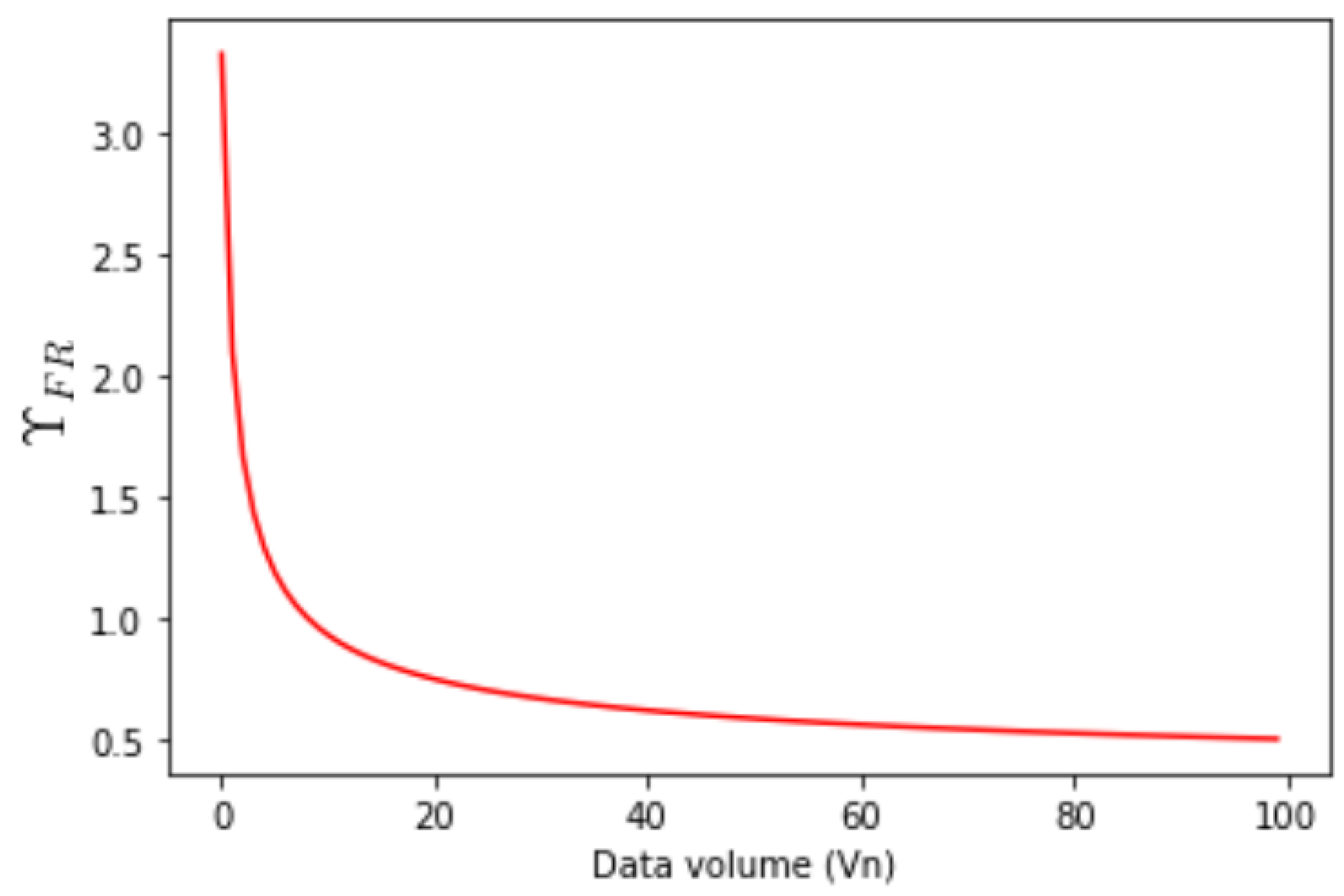
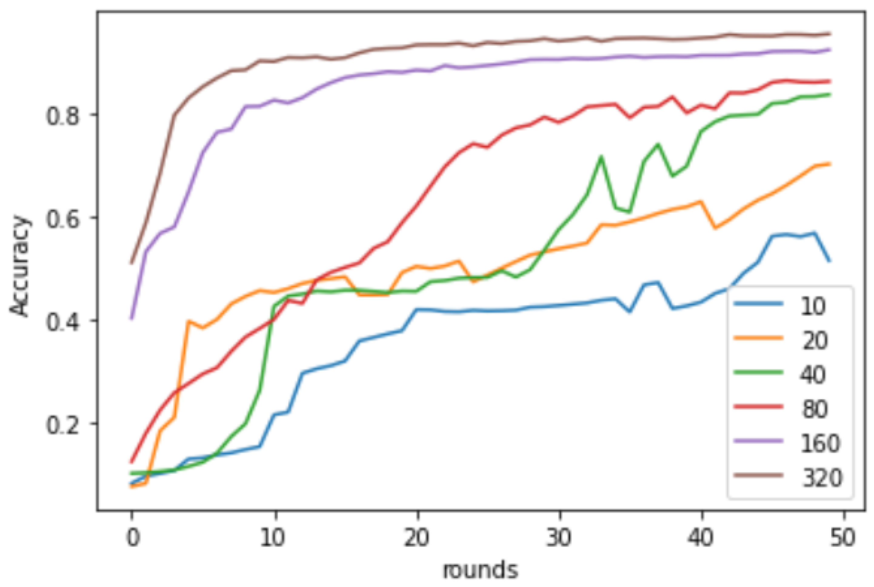
3.4. Effect of Data Volume $V_n$

Figure 8 shows the effect of varying data volume on the performance of FedAvg using the MNIST dataset. We see that for lower volumes of data, the performance is very poor, representing the characteristics of a real-world free rider as a client participating with a very small volume of data. As the data volume is increased, the performance improves, depicting a higher relevance for clients with higher data volume.

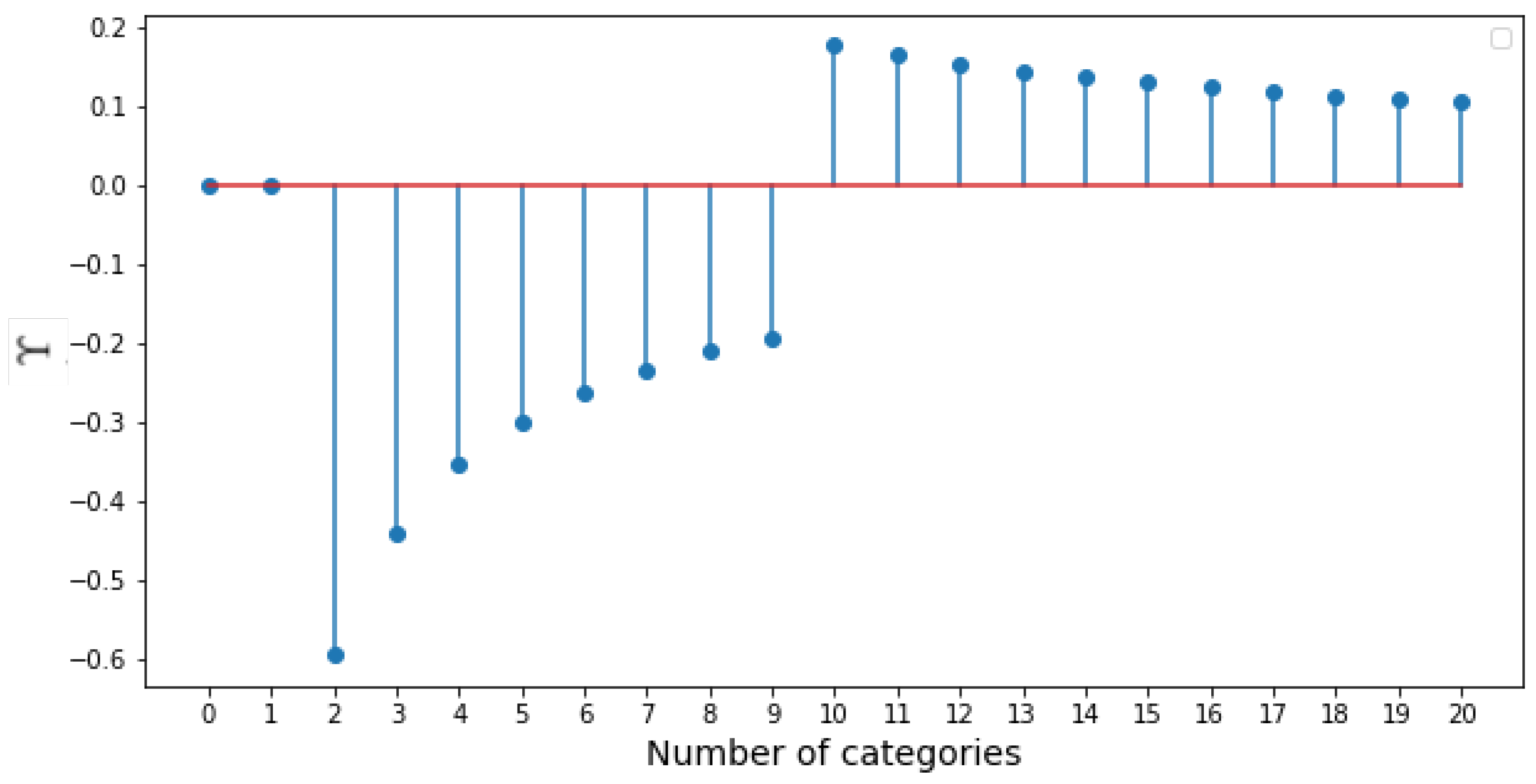
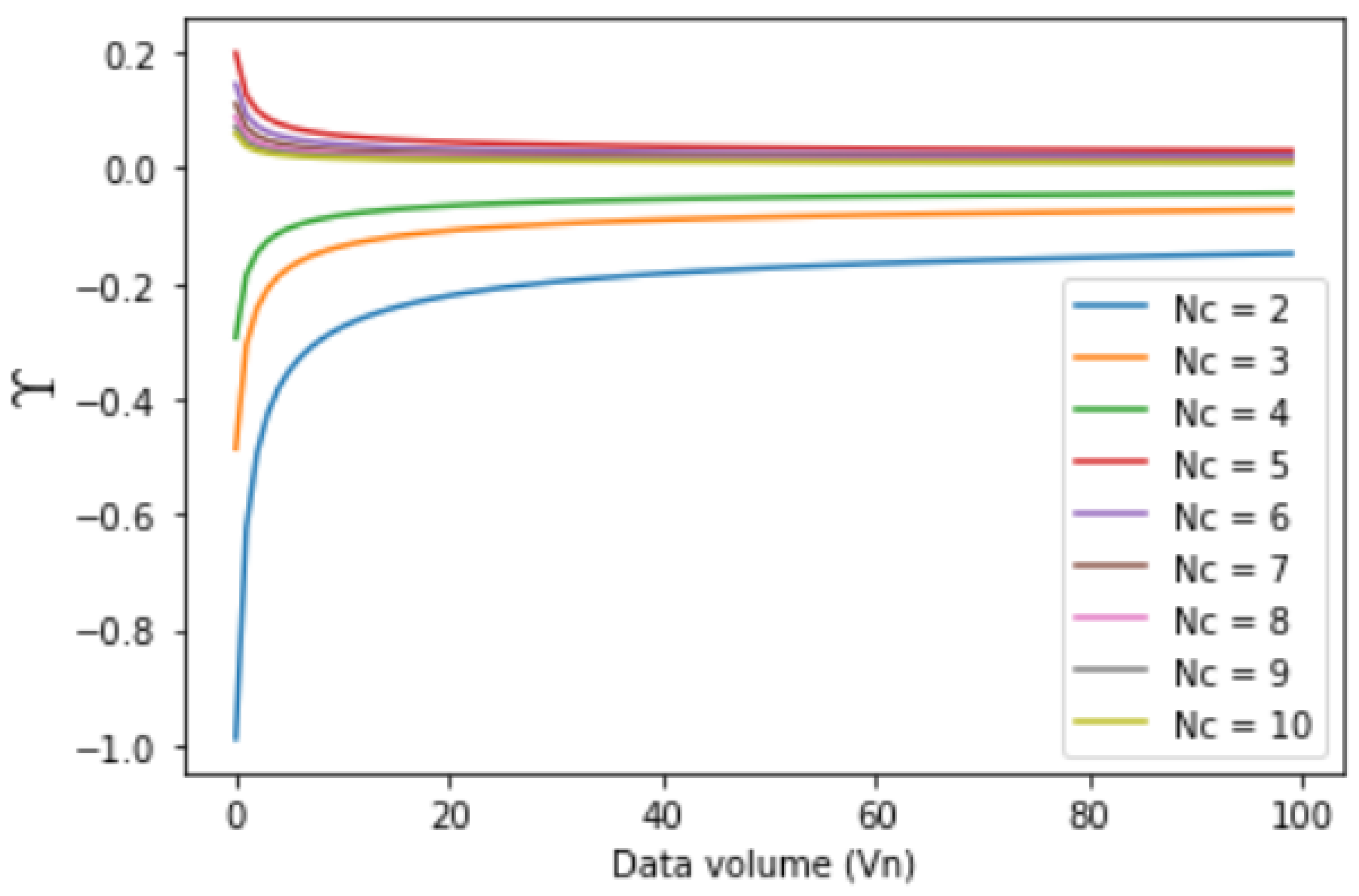
3.5. Effect of Number of Categories $N_c$

The effect of varying the number of categories on clients is shown in Figure 9. Each of the curves correspond to using FedAvg for 15 rounds of refinement using an environment with all clients having $N_c$ number of categories. We can see that clients with a single category perform the poorest and did not learn anything. This explains the $\gamma$ parameter variation, as shown in Figure 7. As the number of clients increases, the performance of FedAvg improves.

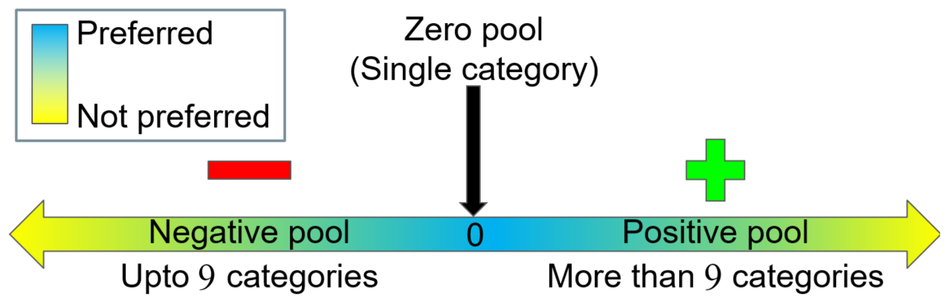
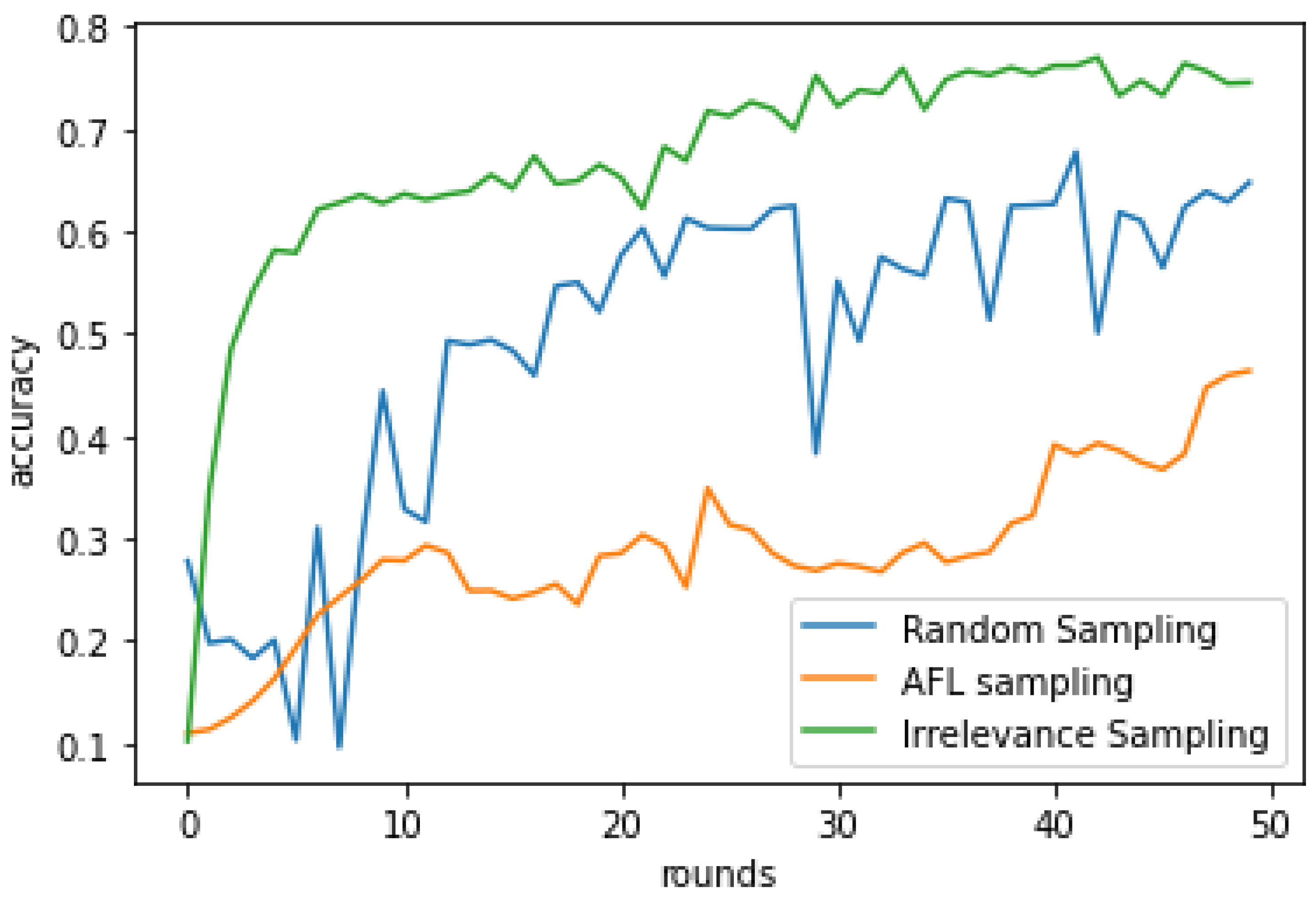
3.6. Highly Skewed Case

We investigated the performance of the three sampling methods on a specially created highly skewed environment using the MNIST dataset. It consists of a few clients with high class imbalance, and moderate free rider repletion is present in the environment. Moreover, three classes of digits 7, 8 and 9 are available with clients having less than three classes only (zero pool and negative pool). This environment shows the importance of the zero pool and negative pool. Figure 10 shows the performance comparison of the three sampling methods in this environment. We can clearly see that the irrelevance sampling method is performing better than AFL and random sampling methods. The parameters used for the irrelevance sampling method are $\alpha =0.5, \beta =0.3, \gamma =0.2$. The smoothness of irrelevance sampling is slightly affected due to the involvement of clients from the zero pool.

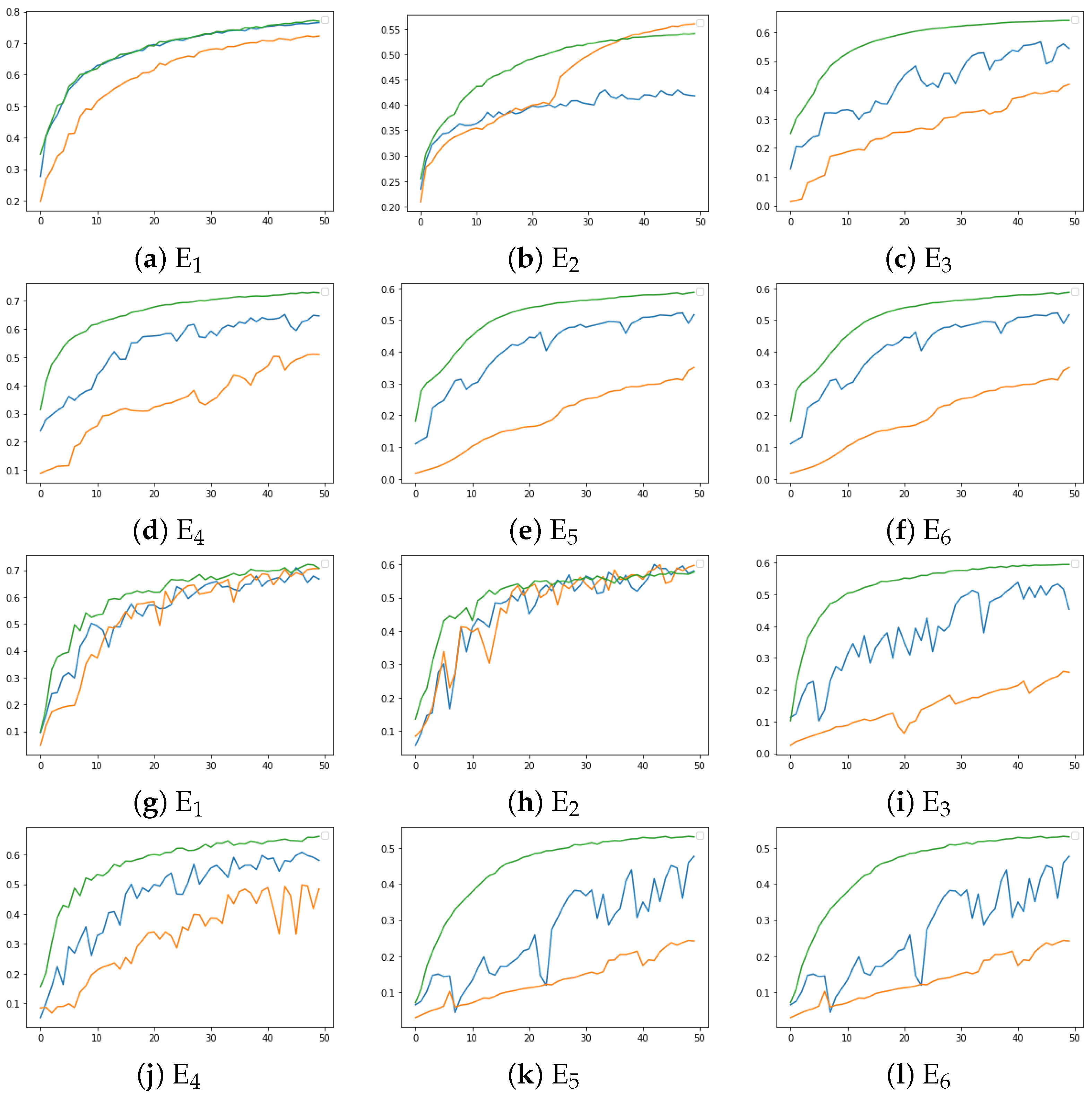
3.7. Convergence Analysis

A convergence analysis is presented in Figure 11 for the FEMNIST dataset for the three sampling methods using the FedAvg learning scheme. Smoother and quicker convergence is observed for the proposed sampling method in comparison with random and AFL sampling for all the environments and under both IID and Non-IID conditions. The results clearly indicate the effectiveness of the proposed method in selecting the optimal subset of clients to update the global model.

4. Observations

4.1. Resistant to Free Riders

Under free rider environments E₃–E₆, the performance of random and AFL sampling methods reduces drastically while the proposed method maintains the top performance across the spectrum.

4.2. Handling Imbalance

The proposed method tries to sample clients with the least degree of imbalance and maximizes the probability of having a set of client models with training experience covering all categories to be included in each iteration of updating the global model. The copies of this updated global model are sent to clients in the next round, and hence, both local and global imbalance is handled. In an extremely imbalanced environment E₂, the performance of the random sampling method reduces drastically while the AFL sampling method handles the imbalance case well. The proposed sampling method handles the imbalance by picking up the clients with the least degree of imbalance and shows an extra edge in performance over the AFL sampling method.

4.3. IID and Non-IID

The proposed sampling method performs at par with the contemporary sampling methods under both IID and Non-IID conditions in all environments E₁–E₆. The C${}_{\gamma }$ clients introduce slight instability but are important in handling highly skewed environments such as covering rare categories from single category clients. There could be a possibility that hard samples are present from C${}_{\gamma }$ clients and hence the parameter $\gamma$ is also of much importance while selecting the parameters of irrelevance sampling. Another case could be that some of the clients are never sampled. In such scenario, it would be useful to select a high fraction of clients based on the irrelevance sampling method and sample the remaining lower fraction randomly. In this way, all clients will become sampled at least once when covered under the random sampling mode.

5. Conclusions

In conclusion, the proposed irrelevance score and the irrelevance sampling strategy is quite robust in a variety of challenging situations, including Non-IID data, a highly imbalanced federated environment and federated environment replete with free-riders. Its versatility is further demonstrated on multiple datasets with varying challenges even when different learning approaches may be employed. Further, the proposed irrelevance score is effective in preserving client privacy. Therefore, the irrelevance score and the proposed sampling method may open new doors of research.

Our experiments use simulations of possible real-world environments. Nonetheless, some specific unexplored environments may pose new challenges. One such challenge is the scenario where the irrelevance score returned by a client is invalid. Another challenge could be a rapid increase in the number of clients coming onto the server (M). Scalability could be an issue, but initially limiting the number of clients coming onto the server depending on the severity of the use case can be a solution. However, these cases are challenges faced by the AFL sampling method as well. Other disguised schemes of free riders are currently out of the scope of the proposed method and future research work is required on this to resolve issues under these scenarios. In the future, we would like to consider more challenging problems, such as clinical-record-based diagnosis using pathology labs as clients in a federated environment.

References

1. Roh, Y.; Heo, G.; Whang, S.E. A survey on data collection for machine learning: A big data—AI integration perspective. IEEE Trans. Knowl. Data Eng. 2018, 33, 1328–1347. [Google Scholar] [CrossRef] [Green Version]
2. Voigt, P.; Bussche, A.v.d. The EU General Data Protection Regulation (GDPR): A Practical Guide, 1st ed.; Springer: Berlin/Heidelberg, Germany, 2017. [Google Scholar]
3. Bonawitz, K.; Eichner, H.; Grieskamp, W.; Huba, D.; Ingerman, A.; Ivanov, V.; Kiddon, C.; Konecný, J.; Mazzocchi, S.; McMahan, H.; et al. Towards federated learning at scale: System design. Proc. Mach. Learn. Syst. 2019, 1, 374–388. [Google Scholar]
4. Kairouz, P.; McMahan, H.; Avent, B.; Bellet, A.; Bennis, M.; Bhagoji, A.; Bonawitz, K.; Charles, Z.; Cormode, G.; Cummings, R.; et al. Advances and open problems in federated learning. arXiv 2019, arXiv:1912.04977. [Google Scholar]
5. Verma, D.C.; White, G.; Julier, S.; Pasteris, S.; Chakraborty, S.; Cirincione, G. Approaches to address the data skew problem in federated learning. In Proceedings of the Artificial Intelligence and Machine Learning for Multi-Domain Operations Applications; 2019; Volume 11006, pp. 542–557. Available online: https://www.spiedigitallibrary.org/conference-proceedings-of-spie/11006/110061I/Approaches-to-address-the-data-skew-problem-in-federated-learning/10.1117/12.2519621.short?SSO=1 (accessed on 25 January 2022).
6. Zhao, Y.; Li, M.; Lai, L.; Suda, N.; Civin, D.; Chandra, V. Federated learning with non-iid data. arXiv 2018, arXiv:1806.00582. [Google Scholar] [CrossRef]
7. Guo, X.; Yin, Y.; Dong, C.; Yang, G.; Zhou, G. On the class imbalance problem. In Proceedings of the Fourth International Conference on Natural Computation, Jinan, China, 18–20 October 2018; Volume 4. [Google Scholar]
8. Asad, M.; Moustafa, A.; Ito, T.; Muhammad, A. Evaluating the communication efficiency in federated learning algorithms. arXiv 2020, arXiv:2004.02738. [Google Scholar]
9. Lin, J.; Du, M.; Liu, J. Free-riders in federated learning: Attacks and defenses. arXiv 2019, arXiv:1911.12560. [Google Scholar]
10. McMahan, H.; Moore, E.; Ramage, D.; Hampson, S.; Arcas, B.A.Y. Communication-efficient learning of deep networks from decentralized data. In Proceedings of the 20th International Conference on Artificial Intelligence and Statistics, Fort Lauderdale, FL, USA, 20–22 April 2017; Volume 54, pp. 1273–1282. [Google Scholar]
11. Konecný, J.; McMahan, H.; Ramage, D.; Richtárik, P. Federated optimization: Distributed machine learning for on-device intelligence. arXiv 2016, arXiv:1610.02527. [Google Scholar]
12. Johnson, R.; Zhang, T. Accelerating stochastic gradient descent using predictive variance reduction. In Proceedings of the Advances in Neural Information Processing Systems, Lake Tahoe, NV, USA, 5–10 November 2013; pp. 315–323. [Google Scholar]
13. Wang, Y. CO-OP: Cooperative Machine Learning from Mobile Devices; University of Alberta: Edmonton, AB, Canada, 2017. [Google Scholar]
14. Nilsson, A.; Smith, S.; Ulm, G.; Gustavsson, E.; Jirstrand, M. A performance evaluation of federated learning algorithms. In Proceedings of the Second Workshop on Distributed Infrastructures for Deep Learning, Quebec, QC, Canada, 7–11 November 2022; pp. 1–8. [Google Scholar]
15. Corinzia, L.; Buhmann, J. Variational federated multi-task learning. arXiv 2019, arXiv:1906.06268. [Google Scholar]
16. Nishio, T.; Yonetani, R. Client selection for federated learning with heterogeneous resources in mobile edge. In Proceedings of the IEEE International Conference on Communications (ICC), Shanghai, China, 20–24 May 2019; pp. 1–7. [Google Scholar]
17. Chen, W.; Horvath, S.; Richtarik, P. Optimal Client Sampling for Federated Learning. arXiv 2020, arXiv:2010.13723. [Google Scholar]
18. Chen, W.; Horvath, S.; Richtarik, P. Adaptive Client Sampling in Federated Learning via Online Learning with Bandit Feedback. arXiv 2021, arXiv:2112.14332. [Google Scholar]
19. Kang, J.; Xiong, Z.; Niyato, D.; Yu, H.; Liang, Y.-C.; Kim, D. Incentive design for efficient federated learning in mobile networks: A contract theory approach. In Proceedings of the IEEE VTS Asia Pacific Wireless Communications Symposium, Singapore, 28–30 August 2019; pp. 1–5. [Google Scholar]
20. Zong, B.; Song, Q.; Min, M.R.; Cheng, W.; Lumezanu, C.; Cho, D.; Chen, H. Deep autoencoding gaussian mixture model for unsupervised anomaly detection. In Proceedings of the International Conference on Learning Representations, Vancouver, BC, Canada, 30 April–3 May 2018. [Google Scholar]
21. Fraboni, Y.; Vidal, R.; Lorenzi, M. Free-rider attacks on model aggregation in federated learning. In Proceedings of the International Conference on Artificial Intelligence and Statistics, Virtual Conference, 13–15 April 2021; pp. 1846–1854. [Google Scholar]
22. Goetz, J.; Malik, K.; Bui, D.T.; Moon, S.; Liu, H.; Kumar, A. Active federated learning. arXiv 2019, arXiv:1909.12641. [Google Scholar]
23. Auger, N.; Jugé, V.; Nicaud, C.; Pivoteau, C. On the worst-case complexity of timsort. arXiv 2018, arXiv:1805.08612. [Google Scholar]
24. Deng, L. The mnist database of handwritten digit images for machine learning research [best of the web]. IEEE Signal Process. Mag. 2012, 29, 141–142. [Google Scholar] [CrossRef]
25. Clanuwat, T.; Bober-Irizar, M.; Kitamoto, A.; Lamb, A.; Yamamoto, K.; Ha, D. Deep learning for classical japanese literature. arXiv 2018, arXiv:1812.01718. [Google Scholar]
26. Cohen, G.; Afshar, S.; Tapson, J.; Schaik, A. EMNIST: Extending MNIST to handwritten letters. In Proceedings of the 2017 International Joint Conference on Neural Networks (IJCNN), Anchorage, AK, USA, 14–19 May 2017. [Google Scholar]
27. Duarte, M.F.; Hu, Y.H. Vehicle classification in distributed sensor networks. J. Parallel Distrib. Comput. 2004, 64, 826–838. [Google Scholar] [CrossRef]
28. Anguita, D.; Ghio, A.; Oneto, L.; Parra, X.; Reyes-Ortiz, J.L. A public domain dataset for human activity recognition using smartphones. In Proceedings of the 21th International European Symposium on Artificial Neural Networks, Computational Intelligence and Machine Learning, Bruges, Belgium, 24–26 April 2013; pp. 437–442. [Google Scholar]
29. Dua:2019 (UCI) Machine Learning Repository. 2017. Available online: https://ergodicity.net/2013/07/ (accessed on 25 January 2022).
30. Nandipati, S.C.R.; Chew, X. Classification and Feature Selection Approaches for Cardiotocography by Machine Learning Techniques. J. Telecommun. Electron. Comput. Eng. (JTEC) 2020, 12, 7–14. [Google Scholar]
Figure 1. Dependence of irrelevance score component Υ FR on data volume ( V n ).
Ai 03 00008 g001
Figure 2. Dependence of irrelevance score component Υ NIID on Number of Categories ( N c ) for a problem with N o = 20 global classes.
Ai 03 00008 g002
Figure 3. Variation of irrelevance score Υ under maximum imbalance condition.
Ai 03 00008 g003
Figure 4. Visualization of the three pools on a irrelevance score for a problem with N o = 20 global classes.
Ai 03 00008 g004
Figure 5. Non-IID condition ( N o = 5 ). No client has all categories. Sampling the best 3 out of 6 clients with α = β = γ .
Ai 03 00008 g005
Figure 6. Variation of irrelevance score Υ with ( Υ CL = 1 ).
Ai 03 00008 g006
Figure 7. Variation of irrelevance sampling parameters α , β and γ .
Ai 03 00008 g007
Figure 8. Performance of FedAvg using random sampling with different data volume ( V n ).
Ai 03 00008 g008
Figure 9. Performance of FedAvg with environement of clients having different number of categories using the MNIST dataset.
Ai 03 00008 g009
Figure 10. Performance comparison on a highly skewed, moderately free rider repleted and class imbalance environment with 3 classes present only on clients with less than 3 categories.
Ai 03 00008 g010
Figure 11. Convergence analysis of different sampling methods. Green: Irrelevance sampling; Blue: Random sampling; Orange: AFL sampling. (af): IID condition and (gl): Non-IID condition. FEMNIST dataset and FedAvg learning schemes are used.
Ai 03 00008 g011