Article

Chinese Comma Disambiguation in Math Word Problems Using SMOTE and Random Forests

1
School of Information Technology in Education, South China Normal University, Guangzhou 510631, China
2
School of Educational Information Technology, Central China Normal University, Wuhan 430079, China
*
Authors to whom correspondence should be addressed.
AI 2021, 2(4), 738-755; https://doi.org/10.3390/ai2040044
Submission received: 23 November 2021 / Revised: 15 December 2021 / Accepted: 17 December 2021 / Published: 20 December 2021

Abstract

:
Natural language understanding technologies play an essential role in automatically solving math word problems. In the process of machine understanding Chinese math word problems, comma disambiguation, which is associated with a class imbalance binary learning problem, is addressed as a valuable instrument to transform the problem statement of math word problems into structured representation. Aiming to resolve this problem, we employed the synthetic minority oversampling technique (SMOTE) and random forests to comma classification after their hyperparameters were jointly optimized. We propose a strict measure to evaluate the performance of deployed comma classification models on comma disambiguation in math word problems. To verify the effectiveness of random forest classifiers with SMOTE on comma disambiguation, we conducted two-stage experiments on two datasets with a collection of evaluation measures. Experimental results showed that random forest classifiers were significantly superior to baseline methods in Chinese comma disambiguation. The SMOTE algorithm with optimized hyperparameter settings based on the categorical distribution of different datasets is preferable, instead of with its default values. For practitioners, we suggest that hyperparameters of a classification models be optimized again after parameter settings of SMOTE have been changed.

1. Introduction

Automatically solving math word problems (MWPs), which dates back to 1960s [1], gains intensive attention from international scholars [2,3]. In a math word problem solver, natural language understanding technologies were adapted to automatically transform MWPs into a structured representation that facilitates quantitative reasoning. The formalized representation is essentially derived from a list of textual propositions within a sentence or several sentence fragments. With reference to the Rhetorical Structure Theory [4], textual propositions in a math word problem can be defined as quantitative discourse units (QDUs) analogically.
In the transformation process, commas serve as an important cue for detecting QDUs in the problem statement of MWPs. In a general way, MWPs can be split into several QDUs by periods (e.g., Mike’s father is 3 times as old as Mike. 4 years ago, he was 4 times older. How old is Mike?). However, it is unsuitable for a comma to be directly regarded as a delimiter among QDUs in MWPs. The main reason is that the comma has diverse syntactic roles and depicts different semantic relations in the narrative [5,6]. The Chinese comma also identifies the boundary of a sentence just as a period, an exclamation point or question mark does [7]. Additionally, sentence fragments surrounding commas express essential relations for understanding the meaning of the sentence [6]. In Chinese MWPs, comma placement among coordinated phrases tends to describe a “whole-part” relation, whereas prosodic relations, such as a pause between two clauses, are also marked with a comma. In this sense, the utility of the Chinese comma is complex and diverse, which leads to comma ambiguity in MWPs. Therefore, comma disambiguation is necessary for detecting QDUs in Chinese MWPs, and it is addressed as a fundamental step towards the fine-grained semantic parsing with the purpose of mapping problem statements into the structured representation.
Developing a supervised or semi-supervised learning model for comma disambiguation benefits a wide range of downstream natural language processing (NLP) applications, such as discourse analysis and machine translation. To recognize loosely coordinated clauses separated by commas, Xue and Yang trained a maximum entropy classifier using the Chinese Treebank and achieved promising results for comma disambiguation [8]. Inspired by Xue’s effort, Xu et al. introduced different features (e.g., semantic information of two words before and after the comma) to establish a hidden Markov model for Chinese sentence segmentation [9]. Building on their previous work, Yang and Xue further implemented subject–predicate features, mutual information features, span features and lexical features to disambiguate the Chinese comma that was viewed as a delimiter of elementary discourse units, in the sense of the Rhetorical Structure Theory [7]. Likewise, Li et al. extracted rich linguistic features to recognize discourse relations with the maximum entropy classifier [10]. Arivazhagan et al. combined syntactic features and semantic features to train an averaged perception classifier for the prediction of comma roles [6]. Towards Chinese–English patent machine translation, rich linguistic information was exploited to identify commas, which facilitated the quality improvement of translation outputs [11].
To sum up, comma disambiguation is generally transformed into a classification problem, and the maximum entropy classifier is the most frequently used method for comma classification. Meanwhile, most of the above-mentioned studies focused on feature construction and selection to improve the performance of the target classifiers on comma disambiguation. However, there is little work on comma disambiguation associated with the imbalanced learning problem. This problem exerts a negative impact on comma disambiguation directly, and further suppresses the effectiveness of downstream NLP applications such as machine translation, syntactic parsing and semantic analysis. Especially, both syntactic parsing and semantic analysis are conducive to fined-grained information extraction from short text, which is a significant part in the process of machine understanding MWPs. Therefore, there is a demand for an effective, reliable and practicable technique to detect ambiguous commas in MWPs whilst coping with the imbalance learning problem.
In this paper, we addressed comma disambiguation in MWPs as an imbalanced binary classification problem and employed the synthetic minority oversampling technique (SMOTE) and random forests to resolve this problem. Firstly, we converted each comma in MWPs into feature vectors, and then dealt with the class imbalance problem based on SMOTE. Secondly, we jointly tuned hyperparameters of SMOTE and random forest classifiers, and subsequently performed comparisons with other classification models, including decision trees, maximum entropy, naïve Bayes and support vector machine. Thirdly, we proposed a novel measure to strictly evaluate the effectiveness of deployed classifiers on comma disambiguation in MWPs. Finally, based on our experimental results, we conclude that random forest classifiers with SMOTE outperform other classification methods in comma classification. Additionally, it is more reliable and acceptable to adopt random forest classifiers rather than alternative methods such as naïve Bayes, maximum entropy and support vector machine to disambiguate commas in MWPs. We also suggest that, when using SMOTE to cope with the class imbalance problem, hyperparameters of classification algorithms should be re-optimized corresponding to the alteration of parameter settings in SMOTE. To the best of our knowledge, this is the first study focused on comma disambiguation in MWPs, which contributes to the field of natural language understanding.

2. Notations and Problem Statement

With the necessity of comma disambiguation for QDUs detection in MWPs, we grouped the Chinese comma into two categories: non-boundary of QDU (non-B-QDU) and boundary of QDU (B-QDU). The categorization of the Chinese comma in MWPs is similar to that used for the recognition of element discourse units [12]. As shown in Figure 1, we observed that class B-QDU significantly outnumbers class non-B-QDU by a large margin. This observation implies that Chinese comma classification is involved in an imbalanced learning problem. Imbalanced learning is defined as a supervised learning process with severe data distribution skews to develop effective decision boundaries between a majority class and a minority class. Preferably, we employed the notation of imbalanced ratio to precisely describe the data skewness between class B-QDU (the majority class) and class non-B-QDU (the minority class). The IR can be computed as the number of the majority divided by the number of the minority. Thus, Chinese comma disambiguation can be cast as an imbalanced binary classification task and mathematically formulated.
We used a Chinese comma dataset derived from a corpus of MWPs and denoted as D = i = 1 n x i ,   y i , where x i is a list of attributes used to represent a comma and class labels of the comma are represented as y i 0 ,   1 , where 0, 1 indicate the class B-QDU, non-B-QDU, respectively. The goal of our task is to construct a standard classification model on the dataset D , which is in essence to figure out a decision model to minimize a loss function that measures the cost of decision error, subject to the imbalanced ratio of the dataset D , denoted as I R D . Its mathematical description is presented as follows:
min f F 1 n x i D L y i ,   f x i + λ Ω f s . t .     I R D = N 0 D N 1 D > 1
where f x i is the decision model, L y i ,   f x i is the loss function, F is a family of decision models dependent upon a parametric space, Ω f is a penalty term measuring the model complexity, λ is a coefficient to weight the empirical risk against the complexity of the decision model and N 0 D and N 1 D are the number of the class B-QDU instances and the number of the class non-B-QDU instances, respectively. Hence, with the purpose of disambiguating Chinese comma in MWPs, we need to refine the imbalanced learning problem through a classification model that is biased toward the class non-B-QDU without sacrificing its performance on the class B-QDU. Class imbalance significantly compromises the performance of most standard learning algorithms, which assume or expect balanced class distributions or equal misclassification costs. Currently, strategies to meet the class imbalance problem have been roughly grouped into sampling, cost-sensitive and active learning methods. Sampling methods can be subdivided into four categories: oversampling, undersampling, informed undersampling and synthetic sampling. In this paper, we employed a synthetic sampling method and random forest classifiers to achieve our goals.

3. Methods

To cope with comma disambiguation in MWPs, we firmly developed an effective method using the SMOTE algorithm and random forest classifiers. In our method, random forest classifiers were built for comma classification in which the imbalanced learning problem was tackled by dint of the SMOTE algorithm. Moreover, we jointly optimized the hyperparameters of the SMOTE algorithm and random forest classifiers to enhance their performance in comma disambiguation. Detailed information about our methods is presented in the following subsections.

3.1. Feature Construction

Comma features automatically obtained from MWPs were categorized into shallow context features, lexical features and phrasal features. Recent studies showed that commas represented as these categories of features are used for comma classification in different NLP tasks. As for machine translation, lexical, phrasal and syntactic features are implemented to train classifiers [11]. Beyond these features, other features such as mutual information features, span features and semantic features are proposed to perform discourse analysis successfully [7]. Admittedly, lexical features as well as phrasal features greatly contributed to a variety of NLP tasks. In practice, both lexical and phrasal features strongly depend on syntactic analysis, but syntactic analyzers such as tokenizers and constituent parsers practicably achieve poor performance in Chinese MWPs. In an attempt to alleviate this concern, it is acceptable to introduce shallow context features besides the lexical and phrasal features. As a result, comma features in our method are summarized as follows:
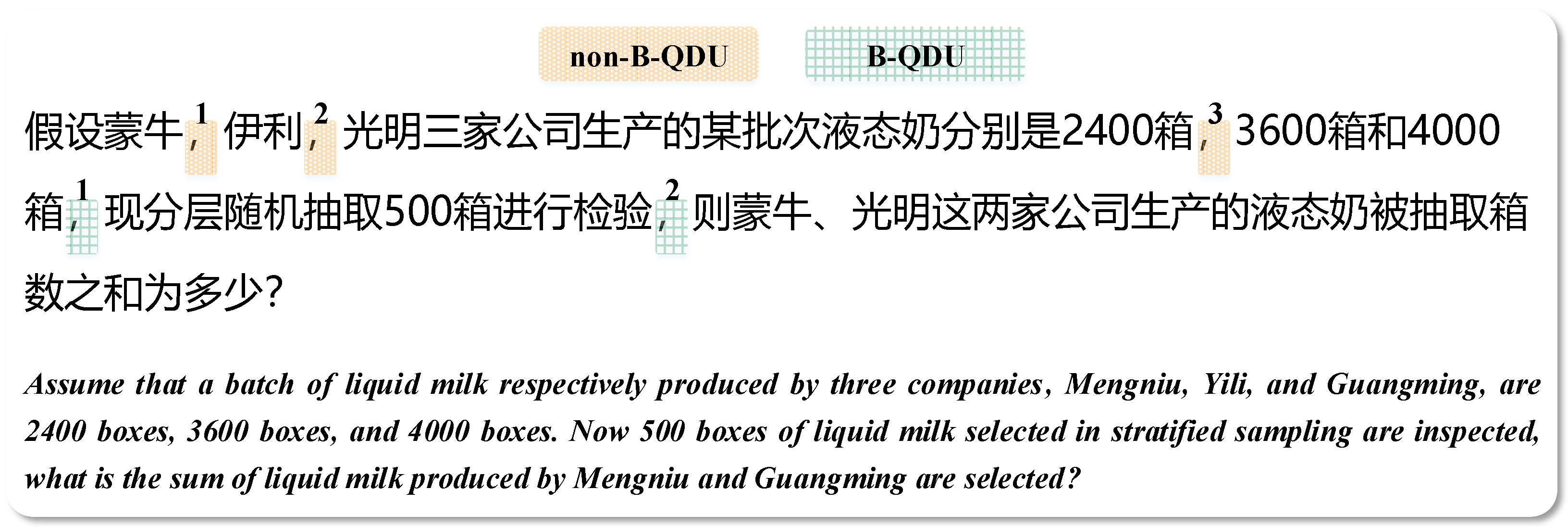
  • Shallow context features refer to the surface information of a text segment before or behind a comma. Given a text segment before a comma, it can be turned into a list of surface features including the position of the comma (PC), the string length (SL), the number of words (NW) and whether it contains numeric or English letters (NoE).
  • Lexical features are of word level and emphasize the part-of-speech (POS) and length of the first word (WL) before or behind a comma.
  • Phrasal features are derived from syntactic constituents of a text segment before or behind a comma. For each textual math word problem, a subject–predicate (SP) structure is identical to simple and unbroken discourse units that can be turned into a set of QDUs. Thus, the number of SP structures was chosen as the essential phrasal feature instead of other phrases such as noun phrase and prepositional phrase.
We implemented a text preprocessor using two attainable steps to construct comma features. During preprocessing, we firstly established word segmentation without stop words filtering, and concurrently performed syntactic parsing on the raw textual MWPs. POS tagging set covers 22 categories, and each category contains some sub-categories [13]. In addition, the syntactic parsing was based on the Penn Chinese Treebank. For the elaboration of the primitive features we constructed, this is best illustrated with an example plotted in Figure 2. Given the numbered commas such as 1, 2 and 3 within the exhibited example, we excavated the primitive features from shallow span, lexical and phrasal levels, and also summarized them in Table 1. Subsequently, the Cartesian product was performed on the primitive features to yield new features. These derived features are loaded with the contextual and syntactical information about the corresponding comma. For instance, given two plain features such as before-NoE (true, false) and behind-NoE (true, false), there might be useful information lying in the induced features (true-false, true-true, false-true, false-false). In short, different categorical features were automatically extracted from the two text spans surrounding a comma through general NLP techniques, and gave access to comma disambiguation in Chinese MWPs.

3.2. SMOTE

The synthetic minority oversampling technique (SMOTE) [14] was employed to solve the imbalanced learning problem in the task of comma disambiguation. SMOTE is a powerful synthetic sampling method and has shown great success in various applications. In theoretical terms, a synthetic sample S based on SMOTE is a linear combination of two similar samples denoted as X and X K from the minority class. The linear combination is expressed as Equation (2), where δ is a random seed between 0 and 1, and X K is a random selection among the K-nearest neighbors of X in the minority class. This is the kernel part of the SMOTE algorithm which is described in Algorithm 1. The similarity among samples was measured based on the Euclidean distance in order to figure out the K-nearest neighbors of X in the minority class. SMOTE is efficient in reducing the class imbalance problem for most classifiers trained on low-dimensional data but failed with high-dimensional data [15]. Despite its failure to perform with high-dimensional datasets, we believe that SMOTE is beneficial to our class imbalance datasets from an empirical point of view.
S = X + δ × X K X
Algorithm 1 SMOTE in Pseudo-code
Input: The minority class in the dataset D m i n , the percentage of synthetic minority class P, and the number of nearest neighbors K
Output: The synthetic samples of minority class Syn
1: if P < 100 then
2:    Randomize the minority class dataset D m i n ;
3:     D m i n = P / 100 × D m i n ;
4:    P = 100;
5: end if
6: Syn is initialized to an array for the synthetic samples of minority class;
7:  P = i n t P / 100 ;
8:  i 0 ;
9: for each d D m i n  do
10:    Compute the K-nearest neighbors D d k for d : D d k D m i n ;
11:    while P ≠ 0 do
12:       Randomize an integer n between 0 and K 1 :   n 0 ,   K 1 ;
13:       Compute the difference between d and D d k n :   d i f D d k n d ;
14:       Randomize a number gap between 0 and 1: g a p 0 ,   1 ;
15:       Generate a synthetic minority: S y n i = d + d i f × g a p ;
16:        i i + 1 ;
17:        P P 1 ;
18:    end while
19: end for
20: return Syn;

3.3. Random Forests

We established random forest classifiers to disambiguate commas in MWPs. In essence, a random forest classifier is a special situation of bagging, which is an ensemble learning to combine prediction from multiple decision trees built on bootstrapped training datasets. As illustrated in Figure 3, the training pipeline of random forest classifiers is separated into three steps: (1) drawing bootstrapped datasets, (2) training a set of classification and regression tree (CART) models, and (3) aggregating all predictions made by CART models.
Firstly, bootstrap sampling was performed to create different training datasets. Bootstrapping is a technique used for drawing training datasets from the original dataset by randomly resampling with replacements. Some samples in the original dataset may be used more than once to construct a decision tree. Theoretically, approximately two-thirds of samples are selected to generate decision trees in the forest, while the rest of samples known as out-of-bag samples can be used to estimate the generalization performance or facilitate the pruning of decision trees.
Secondly, bootstrapped training datasets were fed into a collection of CART models. Each CART classification model is built on a bootstrapped training dataset in a divide-and-conquer way. The root node of CART corresponds to the entire training dataset, and each node of CART is divided into child nodes corresponding to a partitioning of the available dataset under a splitting criterion. In the process of establishing the CART classification model, the splitting criterion is objectively established by introducing the Gini index. As with the intension of entropy, the Gini index is a measure of uncertainty. The Gini index identifies the probability of a misclassified sample that is randomly selected from a dataset; the smaller the Gini index is, the less likely a misclassified sample is. Given a training dataset D = i = 1 N x i ,   y i in which its samples are grouped into M   M 2 categories ( C = m = 1 M c m ), the training dataset D can be represented as D = m = 1 M D c m , where D m is a set of samples belonging to class c m . Thus, the Gini index of the dataset D can be computed as Equation (3), where D and D c m are the number of samples in the dataset D and D c m , respectively. Based on the Gini index, the splitting criterion is that the split attribute should achieve the highest Gini index among all candidate split attributes. As a result, a CART in the forest keeps growing from the bottom up using the splitting criterion. This grown CART divides the training dataset D into a set of region units ( R = k = 1 K R k ), and each region unit R k corresponds to a class c k . Consequently, the generated CART and its loss function on the training dataset D can be described using Equations (4) and (5), respectively, where I · is a characteristic function.
G i n i D = m = 1 M D c m D 1 D c m D = 1 m = 1 M D c m D 2
f x = k = 1 K c k I x R k
L y ,   f x = k = 1 K x R k I y f x
Thirdly, majority voting is applied to reach a final prediction that is the output of a random forest classifier. In the random forest classifier, a collection of CART models denoted as F = t = 1 T f t x contribute with the same amount of predictions for an input sample. These CART models F can be deemed as a committee decision to determine the sample class c i by the majority vote method. In mathematical terms, the collective prediction H x can be represented as Equation (6).
H x = a r g m a x c i 1 T t = 1 T I f t x = c i
The procedure of training random forest classifiers reveals that the diversity of each decision tree results from the randomness of sample bootstrapping and attribute selecting. The randomness increases the otherness among base classifiers, a set of decision trees, and further enhances the generalization performance in the ensemble accordingly. With the exception of suitable performance on generalization, random forest classifiers are not only similar to or better than Adaboost in accuracy and faster than bagging or boosting, but they are also relatively robust to outliers and noise. Taking these strengths into consideration, random forest classifiers have been successfully engaged in a wide variety of practical problems, such as medical informatics [16], cheminformatics [17], ecology [18], geoinformatics [19] and bioinformatics [20]. In particular, random forest classifiers are built from highly imbalanced data for disease risk prediction [21].

3.4. Hyperparameter Tuning

The effectiveness of SMOTE and random forest classifiers is affected by their hyperparameter settings. Optimal hyperparameter settings of random forest classifiers are sensitive to the distribution of the training dataset, while SMOTE is doomed to change the sample size and distribution of the training dataset. It is thus indispensable to optimize all the hyperparameters of SMOTE and random forest classifiers simultaneously.
The hyperparameters of SMOTE are the percentage of synthetic minority class P and the number of nearest neighbors K. Obviously, the parameter space in SMOTE is of the Cartesian product of the parameter settings P and K   ( P × K ). The parameter P relies on the amount of negative and positive samples, and the required balanced rate between the negative and positive samples. With regard to the imbalanced ratio of our experimental datasets, the synthetic minority class in SMOTE was thus incrementally specified as 100, 200, 300, 400 and 500 percent of its original size. As for the number of nearest neighbors K, it is such an awkward setting that we had to randomly assign a value to it. An improper value initiated to the parameter K results in synthesizing minority samples in the region of the majority class, regarded as noise, and further hinders the classification effect correspondingly [22]. In the original SMOTE algorithm [14], the recommended value of parameter K is 5. Nevertheless, parameter K was set to different integer values from 3 to 9 in order to capture an optimal choice.
Likewise, there are two significant hyperparameters named nTrees and nAttrs in random forest classifiers. While increasing the number of trees nTrees, the generalization error converges, and over-training can also be neglected [23]. In other words, the more trees added to the forest, the weaker the tendency of overfitting. On the other hand, random forest classifiers are completely susceptible to the number of randomly investigated attributes nAttrs. Decreasing the nAttrs decreases the correlation among trees in the forest and as well as decreases their strength. The decrease in nAttrs is easily caught in a dilemma that the corresponding decreasing correlation and strength may further lead to adverse effects on the accuracy of random forest classifiers. In this situation, the hyperparameter settings, nTrees and nAttrs, ranged from 5 to 100 with 20 steps and from 1 to 15 with 15 steps, respectively, when we proceeded with hyperparameter tuning.
To achieve a competent random forest classifier, its hyperparameter values must be specified before beginning training. However, it is a complicated and heavy mission to capture an optimal hyperparameter setting, which varies for different datasets. The process of hyperparameter tuning can be roughly divided into three steps: (1) training and evaluating on all hyperparameter settings by hold-out or cross-validation in a loop, (2) seeking out the best hyperparameter setting according to different measure metrics and (3) retraining a classifier on all available dataset (training and validating dataset) under the best hyperparameter setting. At present, hyperparameter tuning methods can be conventionally sorted into more three main categories: grid search, random search and smart search. The grid search method, even in most cases, is expensive in computation time, but seems naïve and can be easily parallelized. It may be a risk to utilize approaches that take advantage of approximations or heuristics to avoid an exhaustive parameter search, and the required computational cost of grid search is not much more than that of smart methods when there are only two hyperparameters to be optimized [24]. Therefore, the grid search method is attractive and available and thus was adopted to optimize the hyperparameters of random forest classifiers.

4. Experimental Setup

As described in Figure 4, the process of our experiments has two stages. The first stage, known as the development of predictive models, was to increase the performance on comma classification by tweaking random forest (RF) classifiers and SMOTE algorithm, and to select the best-performing model from the feature space given by our experimental dataset. To make it more concrete in the first stage, the dataset was split into training data, validation data and test data. We conducted an experiment on the training data and validation data to tune the hyperparameters of SMOTE and RF classifiers simultaneously. Successively, classification algorithms, including decision trees (C4.5), maximum entropy (ME), naïve Bayes (NB) and support vector machine (SVM), were built on training data, and served as baseline models compared to an RF classifier with optimized hyperparameter settings. These baseline models had been successfully applied to identify ambiguous commas for various NLP tasks [7,11]. Accordingly, another experiment was launched on the test data in order to compare the performance achieved by the RF classifier with those by baseline models using different evaluation measures.
All the comma classification models built in the first stage were deployed in the second stage. We intended to estimate their generalization performance on future or live data, and tried to answer a question such as, “Is the RF classifier with SMOTE better than baseline models for comma disambiguation in MWPs?” This question is related to a statistical hypothesis testing. Hence, we hypothesized that the RF classifier with SMOTE leads to a statistically significant improvement in comma disambiguation in MWPs. With this hypothesis testing, an evaluation measure was devised to assess the actual effectiveness of deployed models on comma disambiguation in MWPs. We performed bootstrap sampling on a new dataset, and the bootstrapped datasets were simulated as live data to quantify and compare the performance uncertainty of deployed models based on the proposed evaluation measure.
All experiments were conducted in WEKA, an open source machine learning library in Java [25], on a Dell laptop with 2 GHz Intel Core i7 CPU and 8 GB of memory. Information about our experimental datasets and evaluation measures is detailed in Section 4.1 and Section 4.2 respectively.

4.1. Dataset Description

Concerning comma disambiguation in MWPs, there is, to our knowledge, no benchmark corpus for this goal in published scientific literature. On this occasion, we built a raw dataset concerned with Chinese comma disambiguation in MWPs. Each math word problem in this unsorted raw dataset is about stratified sampling. These textual problems were collected from Chinese college entrance mathematics exams of the past ten years and two mathematic educational websites. Each comma in 263 MWPs was manually annotated as class B-QDU or non-B-QDU. Consequently, the human-annotated dataset, which we called CODIS, consisted of 1184 commas. There were 172 positive samples with an identical label non-B-QDU and 1012 negative samples with another label. In the experimental process, the CODIS dataset was split into a training dataset with 710 samples, a validation dataset with 237 samples to tune hyperparameters and a test dataset with 237 samples to compare the generalization ability of our method with the baseline methods on different metrics. Moreover, another dataset with 100 MWPs was constructed and named APP-CODIS. In the APP-CODIS dataset, each MWP was absent from the CODIS dataset, and served as live data to evaluate the performance of deployed classifiers on comma disambiguation.

4.2. Evaluation Measures

For imbalanced learning problems, overall classification accuracy might not be an adequate evaluation metric because the predictive accuracy is biased towards the majority class. In this paper, the metrics we employ to compare the performance among the classifiers include Recall (R), F-measure (F), True Positive Rate (TPR), True Negative Rate (TNR), Weighted Accuracy (WA), G-mean (GM), and Matthews Correlation Coefficient (MCC). These metrics have been widely used to evaluate the performance of classification algorithms on class imbalance data [26,27].
Recall and F-measure have been commonly adopted in the realm of information retrieval. A desirable classifier built from an imbalanced dataset should be capable of achieving high prediction accuracy for the majority and reasonable accuracy for the minority. With this desire, the weighted accuracy was proposed [28] and computed as Equation (7), in which different weights are specified to TPR and TNR in order to compensate for the bias in the imbalanced dataset. The adjustable weight of TPR is commonly set to 0.5, which means that the importance of prediction accuracy on the minority is equal to that on the majority. Moreover, we used the MCC as another measure to assess classification performance on our class imbalance datasets. MCC takes mutual accuracies and error rates on all classes into consideration and hence is less influenced by imbalanced dataset [29]. Additionally, a receiver operating characteristic (ROC), a two-dimensional graph known as an ROC curve, was employed to illustrate the performance of classifiers. The ROC curve and its area under curve (AUC) have proven to be credible performance metrics as they are insensitive to diversifications of class distribution [20,30].
W A = β × T P R + 1 β × T N R
S A = n = 1 N m = 1 M I H x n m = y n m N
Since commas are regarded as delimiters among quantitative discourse units (QDUs) in a math word problem, it makes sense to measure the accuracy of deployed classifiers to detect ambiguous commas in the word problem. This means that only when all commas have been correctly classified can the math word problem be accurately segmented into a list of QDUs. We thus propose a practical and strict measure to evaluate the performance of deployed classifiers on the APP-CODIS dataset. The proposed measure herein is capable of highlighting the strict accuracy (SA) of deployed classifiers on comma disambiguation, which also meets the demand of applications in production settings. Suppose that there are N textual problems in the APP-CODIS dataset, and each textual problem has M commas that need to be disambiguated. The computation of SA for a deployed classification model H x is shown in Equation (8), where x n m is a feature vector of the m-th comma in the n-th MWP, y n m is the actual class of comma x n m and I · is a characteristic function.

5. Results and Discussion

In this section, we present experimental results to select optimal hyperparameters for SMOTE and RF classifiers and compare the performance of RF classifiers with baseline methods. We show that the combination of random forest classifiers and the algorithm SMOTE is competitive against alternative methods in comma disambiguation. The details of the experimental results are summarized in the following subsections.

5.1. Selection of Optimal Hyperparameters

Table 2 shows the performance of optimized RF classifiers and its corresponding hyperparameter settings of SMOTE on the validation dataset. This table gives a general view of the performance of optimized RF classifiers on evaluation metrics, including TPR, TNR, WA, GM, MCC and AUC. Standard deviations of these performance metrics were less than 4.5%, indicating that classification performances achieved by the optimal RF classifiers do not have significant variation. That is, no matter what the hyperparameter settings of SMOTE are, the performances of its corresponding optimal RF classifiers turn out smoothly.
For more specific insight into the entire distribution of classification performance after tuning hyperparameters, three plot comparisons of classification performance on TPR and TNR are shown in Figure 5, Figure 6 and Figure 7. We excluded other performance metrics such as MCC, AUC, WA and GM by taking two aspects into consideration: (1) we emphasized classifiers’ performance on positive and negative samples under diverse hyperparameter settings of SMOTE and RF; and (2) both WA and GM are determined by TPR and TNR. A line and scatter plot with an error bar in Figure 5 show the overall fluctuation trends of optimal RF classifiers’ performance on TPR and TNR. As illustrated in Figure 5, the performances on TPR achieved by optimal RF classifiers are more sensitive to parameter settings of SMOTE than on TNR. Boxplots in Figure 6 and Figure 7, where short dash lines signify the mean values of performance metrics, allow for a clear comparison of performance on TPR and TNR at various points in the distribution. For instance, boxplots in Figure 6A clearly exhibit that the TPR distribution at P = 400 is much more favorable than that at P = 100 . More specifically, the 25th, 50th and 75th percentiles of the TPR distribution at P = 400 are much larger than those at P = 100 .
Through the integral analysis of hyperparameter tuning results seen in Table 2 and Figure 5, Figure 6 and Figure 7, we acquired four other observations, summarized as follows:
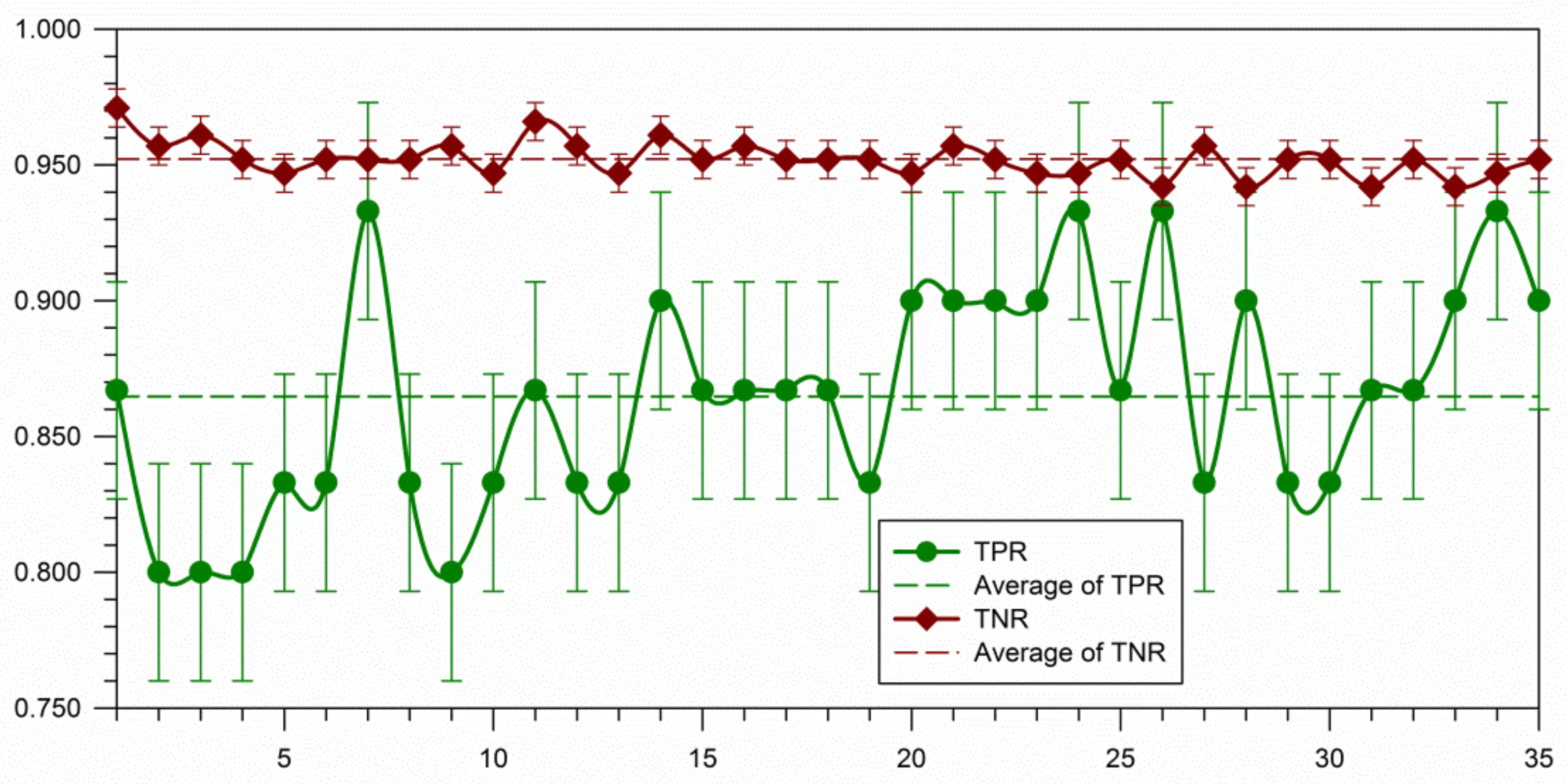
  • AUC values in Table 2 imply that there is no significant variation in the performance of optimal RF classifiers under different parameter settings of SMOTE; in all cases, the hyperparameters of RF are adaptable for obtaining considerable performance, especially the values of nTrees, which range from 20 to 100, while nAttrs are of convergence in 1, 2 or 4. The optimal numbers of nTrees and nAttrs differ from their default values in many applications of RF [31]. For the convergence of nAttrs, it is in line with a thorough investigation claiming that this hyperparameter has a minor impact on the performance, though larger values may be associated with a reduction in the predictive performance [32]. While using MCC to measure performance, optimal RF classifiers achieve a completely acceptable performance.
  • The hyperparameter settings of SMOTE have more influence on the variation of TPR than that of TNR. It may ascribe the flaw of SMOTE in which the synthetic samples derived from the minority samples may be of repeatability, noisy or even fuzzy boundaries between the minority and majority classes [33]. Although there is no apparent variation in TNR in all the cases, classification performance for negative samples tends to be hampered slightly. Thus, the SMOTE adds essential information to the original dataset that enhances RF classifiers’ performance on the minority samples, but is also likely to reduce the performance on classifying the majority samples.
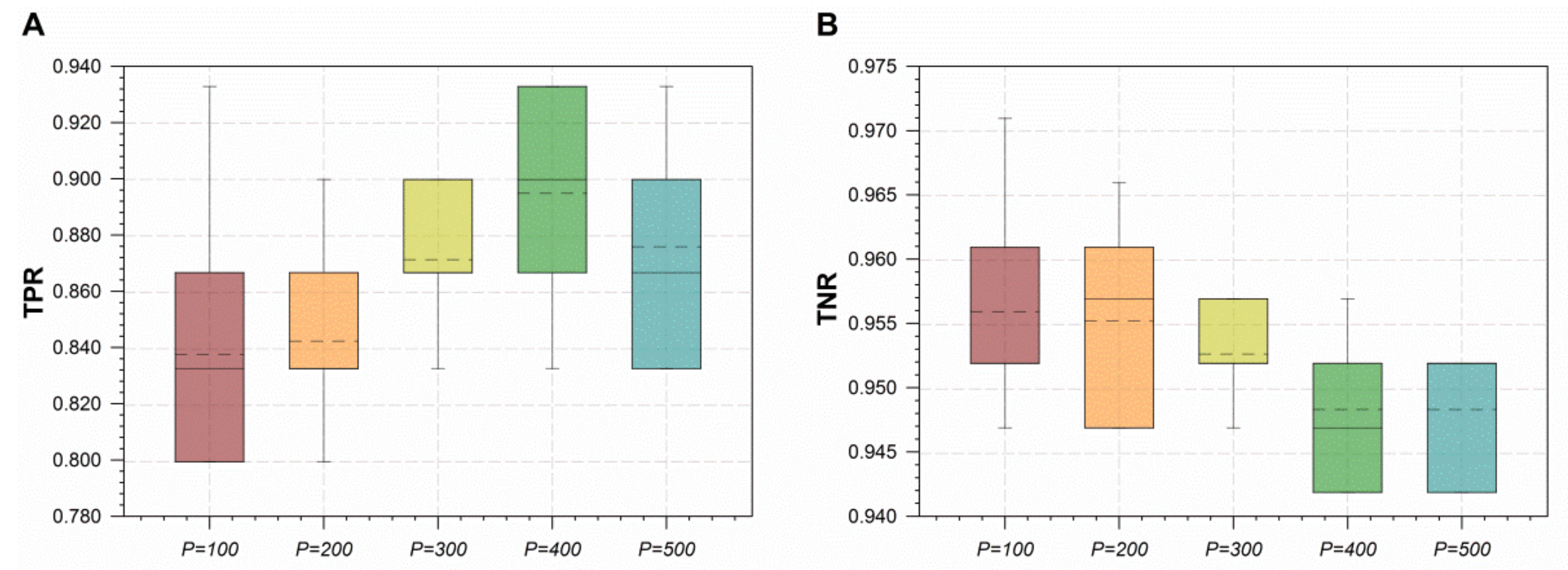
  • Comparing the TPR performance achieved by optimal RF classifiers at P = 400 and P = 100 , there is a statistically significant difference ( p = 0 . 028 at 95% confidence). For the performance on TPR, optimal RF classifiers were improving when P was increasing from 100 to 400. TNR values, corresponding to the rise in P, are depressed, but still significantly considerable. Figure 6 shows that the best performance tradeoff between TPR and TNR occurred at P = 400 . The training dataset augmented by SMOTE ( P = 400 ) was almost fully balanced and induced an optimal RF classifier, achieving the best performance on TPR. It is consistent with the experimental finding that the best oversampling rate made the enlarged dataset fully balanced in order to detect as many positive diabetes patients as possible [34].
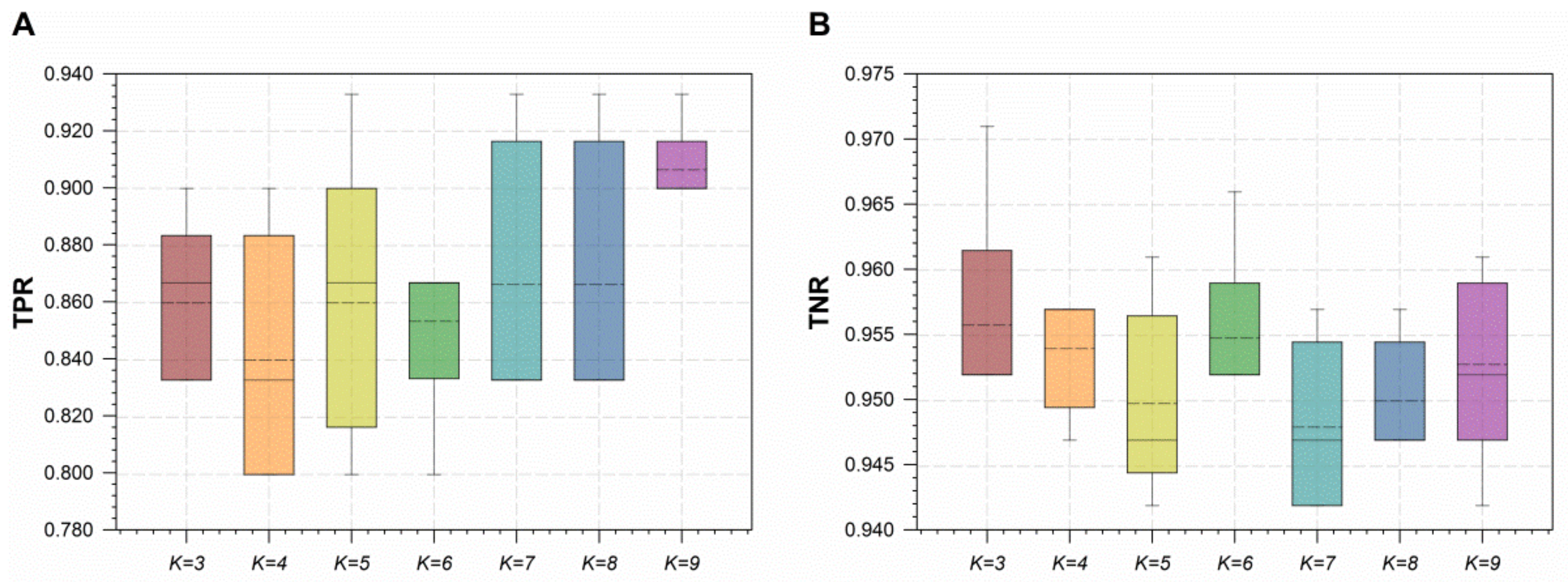
  • As shown in Figure 7, optimal RF classifiers built at K = 9 achieved better performance on TPR without sacrificing the performance on TNR. In spite of parameter P values, parameter K has slightly more influence on the classification of negative samples since the number of negative samples in a training dataset has no change after conducting SMOTE with the diversity of parameter P values. This observation is not compatible with the literature recommendations in which the number of nearest neighbors for SMOTE is set to five [14].
Figure 5. Fluctuation trends of optimal random forest classifiers’ performance on TPR and TNR.
Ai 02 00044 g005
Figure 6. Boxplots of optimal random forest classifiers’ performance on TPR (A) and TNR (B) under different settings of parameter p in the SMOTE algorithm.
Ai 02 00044 g006
Figure 7. Boxplots of optimal random forest classifiers’ performance on TPR (A) and TNR (B) under different settings of parameter K in the SMOTE algorithm.
Ai 02 00044 g007
Based on these observations, the optimal parameter setting of SMOTE is ( P ,   K ) = ( 400 ,   9 ) and the corresponding optimal hyperparameter setting of RF classifiers is ( nTrees ,   nAttrs ) = ( 40 ,   1 ) . These optimized parameter settings were further used to retrain optimal RF classifiers and compare their performance on the test dataset with baseline models.

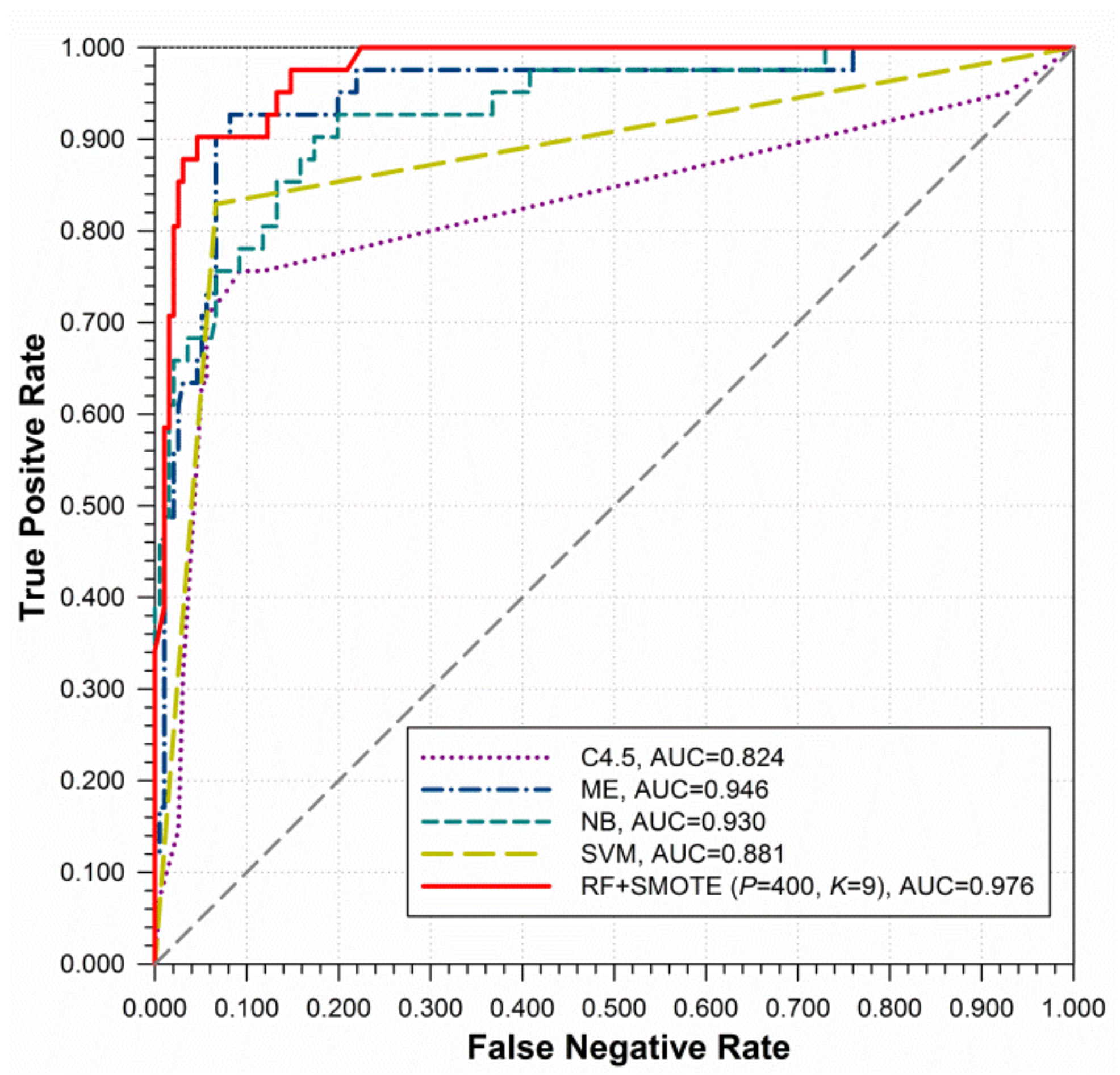
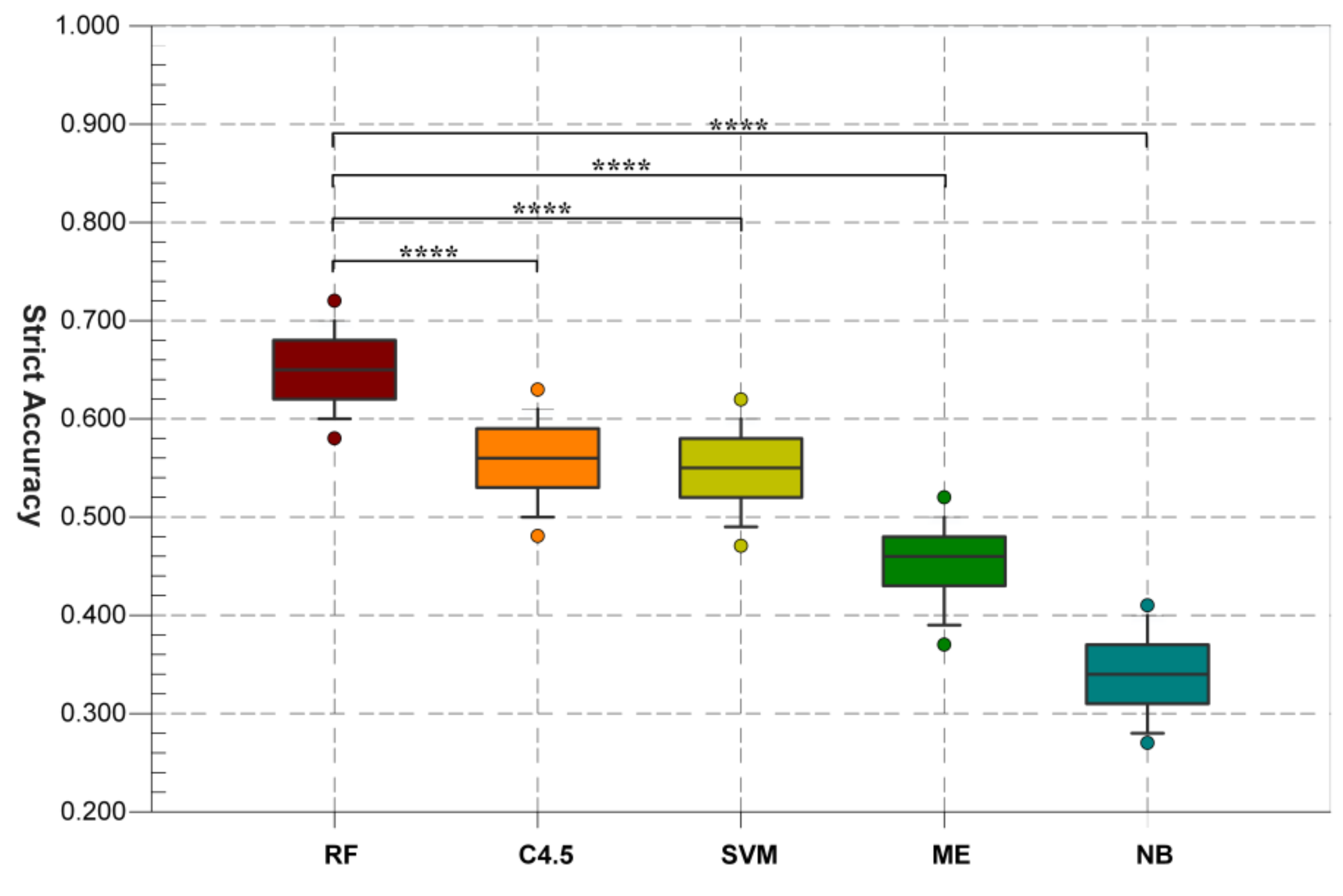
5.2. Comparison of Random Forests and Baseline Models on Comma Classification

To evaluate the efficacy of RF and SMOTE in the context of comma classification, the performance results achieved by RF classifiers were compared with those of baseline models. Before comparisons, all models were to perform hyperparameter tuning based on the grid search method. Subsequently, these optimized classifiers were evaluated on the test dataset, and their performance results are presented in Table 3.
Overall, comparison results in Table 3 show that RF classifiers produce a higher level of classification results on all evaluation measures, whereas SVM achieves the best performance in TPR at 0.829 with a rational TNR at 0.934, but has the second lowest area under the ROC curve (AUC) at 0.881. Unlike the SVM classifier, the NB classifier has the highest TNR at 0.980 but the lowest TPR at 0.610. Both the AUC in Table 3 and the ROC curve in Figure 8 indicate that RF classifiers with the algorithm SMOTE outperform the baseline models. Furthermore, the performances achieved by RF classifiers with different sampling techniques are quite diverse, as shown in Table 3. The performance of RF classifiers with undersampling is inferior to that of RF classifiers with or without SMOTE. A possible explanation for this is that undersampling removes instances from the majority class and thus causes RF classifiers to miss important concepts pertaining to the majority class [35]. With the aid of the SMOTE algorithm, the performance of the RF classifier on TPR improves by 3.2% when the parameter setting was set to ( n T r e e s = 40 ,     n A t t r s = 1 ,     P = 400 ,     K = 9 ), though the performance in AUC also depressed slightly. This observation implies that RF classifiers could have better performance on TPR, WA and GA when the training dataset was fully balanced by SMOTE. These findings are consistent with those of Blagus and Lusa [14], who concluded that SMOTE is efficient in reducing the class imbalance problem with low-dimensional features.
Based on these results, we concluded that RF classifiers with SMOTE comprise the best overall classifier compared to other alternatives in comma classification. Similar conclusions have been reached on the comparison of RF classifiers with other popular classification techniques in a variety of fields. For instance, in the quantitative analysis of civil war, RF classifiers offer superior predictive power compared to several forms of logistic regression [36]; for predicting highly imbalanced data, RF classifiers outperformed SVM, bagging and boosting in terms of ROC and AUC [20,37,38]. Additionally, ME and NB classifiers have been used to automatically disambiguate Chinese commas for different tasks of NLP, but consequently demonstrated relative underperformance on comma classification in MWPs.

5.3. Comparison of Deployed Models on Comma Disambiguation

For the comparison of deployed models on comma disambiguation in MWPs, we acquired 200 bootstrapped datasets from the APP-CODIS dataset. In each bootstrapped dataset, there were 100 MWPs used to measure the strict accuracy (SA) of deployed classifiers at comma disambiguation. It turned out that either the deployed RF or baseline models rigidly produced 200 SA scores in the detection of ambiguous commas. Standard deviations of these SA scores generated by deployed classifiers are at the same level, about 0.04. Figure 9 depicts an average of SA scores for each deployed classification model. Specifically, RF classifiers performed best at SA scores by ( 0.649 ± 0.042 ). To assess the difference between RF classifiers and the baseline models in terms of performance at SA scores, we conducted Mann–Whitney rank sum tests (at 95% confidence) on these SA scores that had failed to pass the normality test (all the p-values are less than 0.05 at 95% confidence). All the p-values produced by the rank sum test re plotted in Figure 9. Statistically significant differences between RF classifiers and alternative methods for comma disambiguation can be observed from Figure 9. Compared with SVM, the mean of SA scores gained by RF classifiers significantly improved by 10%. The average SA score of NB is the worst classifier and compares poorly, with a 30.9% difference from RF classifiers ( p   <   0 . 001 ).
With reference to these comparative results, we confirmed that using a RF classifier with SMOTE for comma disambiguation in MWPs was more reliable and acceptable than alternative methods such NB, ME and SVM. From a practical perspective, the combination of RF classifiers and SMOTE has reached moderate and considerable accuracy in identifying ambiguous commas in MWPs.

6. Conclusions and Future Work

Comma disambiguation is certainly conducive to machine understanding Chinese MWPs. In this paper, we began with the aim of comma disambiguation in MWPs by taking class imbalance learning into consideration. To the best of our knowledge, this is the first study related to comma disambiguation in Chinese MWPs. Comma disambiguation in MWPs can be transformed into a binary classification problem in essence. Such a problem involves in the class imbalance learning with a fundamental issue of how to improve the performance of learning algorithms on the minority classes. We thus employed the SMOTE algorithm and random forests to disambiguate commas in MWPs. The hyperparameters of SMOTE and random forest classifiers were optimized by means of the grid search method. Moreover, we proposed a strict measure to evaluate the performance of deployed classification models on comma disambiguation in Chinese MWPs. Our experimental results implied that random forest classifiers with SMOTE gained a considerable performance in comma disambiguation. Our experimental results also provided evidence of the idea that it is more preferable to use the SMOTE algorithm, tuning its hyperparameters based on the categorical distribution of different datasets, rather than directly using the default parameter values. Another noteworthy finding is that hyperparameters of a classification models should be optimized again after parameter settings of SMOTE have been changed.
To the best of our knowledge, this is the first study addressing comma disambiguation in math word problems, particularly taking the imbalanced learning problem into consideration. Future research can use quantitative discourse units identified in the present study to trace and evaluate students’ cognitive process of solving math word problems. Additionally, the present study develops a practicable methodology that contributes to the hotspot of machine understanding MWPs. Therefore, based on the use of MWPs as a data source, researchers can propose more effective approaches to find insights and linguistic patterns for natural language understanding. With regard to practical implications of our findings, practitioners can use comma disambiguation to identify quantitative discourse units in MWPs, so as to establish an intelligent agent for automatically fine-grained machine understanding MWPs not only at the technical level, but also at educational level.
Notwithstanding its findings and implications, several limitations should be considered. Firstly, our datasets are confined to math word problems about stratified sampling at the high school level, which are more ambiguous than primary school math word problems. Secondly, our datasets are of a suitable size, but may not contain as much information on commas as possible. The larger the datasets, the better the generalization capacity of classifiers are. However, manually labeling numerous commas in MWPs is time-consuming and expensive. Finally, comma features consist of shallow context features, lexical features and phrasal features, and one of the drawbacks is the absence of semantic information. Taking directional cues from these limitations, further research must be conducted to explore active learning methods used for comma disambiguation, as detailed annotation of numerous commas in MWPs can be tedious and even redundant.

Author Contributions

Conceptualization, Q.L.; methodology, J.H.; resources, L.W. and J.H.; writing—original draft preparation, J.H. and Q.L.; writing—review and editing, L.W. and Y.Z.; visualization, J.H.; supervision, Y.Z.; project administration, J.H.; funding acquisition, Q.L. All authors have read and agreed to the published version of the manuscript.

Funding

This work was supported by China Postdoctoral Science Foundation under grant no. 2021M701273 and the National Natural Science Foundation of China under grant no. 61772012.

Institutional Review Board Statement

Not applicable.

Informed Consent Statement

Not applicable.

Data Availability Statement

JimSow/CommaClassification. Available online: https://github.com/JimSow/CommaClassification (accessed on 15 December 2021).

Acknowledgments

The authors would like to thank the anonymous reviewers for their constructive comments, which greatly helped to improve this paper.

Conflicts of Interest

The authors declare no conflict of interest.

References

  1. Bobrow, D.G. Natural Language Input for a Computer Problem Solving System. Ph.D. Thesis, Massachusetts Institute of Technology, Cambridge, MA, USA, 1964. [Google Scholar]
  2. Mukherjee, A.; Garain, U. A review of methods for automatic understanding of natural language mathematical problems. Artif. Intell. Rev. 2008, 29, 93–122. [Google Scholar] [CrossRef]
  3. Zhang, D.; Wang, L.; Zhang, L.; Dai, B.T.; Shen, H.T. The gap of semantic parsing: A survey on automatic math word problem solvers. IEEE Trans. Pattern Anal. Mach. Intell. 2019, 42, 2287–2305. [Google Scholar] [CrossRef] [Green Version]
  4. Mann, W.C.; Thompson, S.A. Rhetorical structure theory: Toward a functional theory of text organization. Text Talk 1988, 8, 243–281. [Google Scholar] [CrossRef]
  5. Kazawa, H.; Isozaki, H.; Maeda, E. NTT Question Answering System in TREC 2001. In Proceedings of the 10th Text Retrieval Conference, Gaithersburg, MD, USA, 13–16 November 2001. [Google Scholar]
  6. Arivazhagan, N.; Christodoulopoulos, C.; Roth, D. Labeling the semantic roles of commas. In Proceedings of the 30th AAAI Conference on Artificial Intelligence, Phoenix, AZ, USA, 14–17 February 2016. [Google Scholar]
  7. Yang, Y.; Xue, N. Chinese Comma disambiguation for discourse analysis. In Proceedings of the 50th Annual Meeting of the Association for Computational Linguistics, Jeju, Korea, 8–14 July 2012. [Google Scholar]
  8. Xue, N.; Yang, Y. Chinese sentence segmentation as comma classification. In Proceedings of the 49th Annual Meeting of the Association for Computational Linguistics: Human Language Technologies, Portland, OR, USA, 19–24 June 2011. [Google Scholar]
  9. Xu, S.; Kong, F.; Li, P.; Zhu, Q. A Chinese sentence segmentation approach based on comma. In Proceedings of the 13th Chinese Lexical Semantics Workshop, Wuhan, China, 6–8 July 2012. [Google Scholar]
  10. Li, X.; Yang, H.; Huang, J. Maximum entropy for Chinese comma classification with rich linguistic features. In Proceedings of the 3th CIPS-SIGHAN Joint Conference on Chinese Language Processing, Wuhan, China, 20–21 October 2014. [Google Scholar]
  11. Li, H.; Zhu, Y. Classifying Commas for Patent Machine Translation. In Proceedings of the 12th China Workshop on Machine Translation, Urumqi, China, 25–26 August 2016. [Google Scholar]
  12. Kong, F.; Zhou, G. A CDT-styled end-to-end Chinese discourse parser. ACM Trans. Asian Lang. Inf. Process. 2017, 16, 1–17. [Google Scholar] [CrossRef]
  13. ICTPOS3.0. Available online: http://www.nlpir.org/wordpress/attachments/2011/06/ICTPOS3.0.doc (accessed on 12 October 2021).
  14. Chawla, N.V.; Bowyer, K.W.; Hall, L.O.; Kegelmeyer, W.P. SMOTE: Synthetic minority over-sampling technique. J. Artif. Intell. Res. 2002, 16, 321–357. [Google Scholar] [CrossRef]
  15. Blagus, R.; Lusa, L. SMOTE for high-dimensional class-imbalanced data. BMC Bioinform. 2013, 14, 106. [Google Scholar] [CrossRef] [PubMed] [Green Version]
  16. Gray, K.R.; Aljabar, P.; Heckemann, R.A.; Hammers, A.; Rueckert, D. Random forest-based similarity measures for multi-modal classification of alzheimer’s disease. Neuroimage 2013, 65, 167–175. [Google Scholar] [CrossRef] [PubMed] [Green Version]
  17. Jayaraj, P.B.; Ajay, M.K.; Nufail, M.; Gopakumar, G.; Jaleel, U.C.A. GPURFSCREEN: A GPU based virtual screening tool using random forest classifier. J. Cheminform. 2016, 8, 1–10. [Google Scholar] [CrossRef] [Green Version]
  18. Oliveira, S.; Oehler, F.; San-Miguel-Ayanz, J.; Camia, A.; Pereira, J.M. Modeling spatial patterns of fire occurrence in Mediterranean Europe using multiple regression and random forest. For. Ecol. Manag. 2012, 275, 117–129. [Google Scholar] [CrossRef]
  19. Rodriguez-Galiano, V.F.; Ghimire, B.; Rogan, J.; Chica-Olmo, M.; Rigol-Sanchez, J.P. An assessment of the effectiveness of a random forest classifier for land-cover classification. ISPRS J. Photogramm. Remote Sens. 2012, 67, 93–104. [Google Scholar] [CrossRef]
  20. Stephan, J.; Stegle, O.; Beyer, A. A random forest approach to capture genetic effects in the presence of population structure. Nat. Commun. 2015, 6, 1–10. [Google Scholar] [CrossRef] [PubMed] [Green Version]
  21. Khalilia, M.; Chakraborty, S.; Popescu, M. Predicting disease risks from highly imbalanced data using random forest. BMC Med. Inform. Decis. Mak. 2011, 11, 51. [Google Scholar] [CrossRef] [Green Version]
  22. Yun, J.; Ha, J.; Lee, J.S. Automatic Determination of Neighborhood Size in SMOTE. In Proceedings of the 10th International Conference on Ubiquitous Information Management and Communication, Danang, Vietnam, 4–6 January 2016. [Google Scholar]
  23. Breiman, L. Bagging predictors. Mach. Learn. 1996, 24, 123–140. [Google Scholar] [CrossRef] [Green Version]
  24. Hsu, C.W.; Chang, C.C.; Lin, C.J. A practical guide to support vector classification. BJU Int. 2008, 101, 1396–1400. [Google Scholar]
  25. Witten, I.H.; Frank, E.; Hall, M.A.; Pal, C.J. Data Mining: Practical Machine Learning Tools and Techniques; Elsevier: Amsterdam, The Netherlands, 2016; pp. 1–621. [Google Scholar]
  26. Department of Statistics. Using Random Forest to Learn Imbalanced Data. Available online: https://statistics.berkeley.edu/tech-reports/666 (accessed on 12 October 2021).
  27. Wu, Q.; Ye, Y.; Zhang, H.; Ng, M.K.; Ho, S.S. ForesTexter: An efficient random forest algorithm for imbalanced text categorization. Knowl.-Based Syst. 2014, 67, 105–116. [Google Scholar] [CrossRef]
  28. Cohen, G.; Hilario, M.; Sax, H.; Hugonnet, S.; Geissbuhler, A. Learning from imbalanced data in surveillance of nosocomial infection. Artif. Intell. Med. 2006, 37, 7–18. [Google Scholar] [CrossRef]
  29. Baldi, P.; Brunak, S.; Chauvin, Y.; Andersen, C.A.; Nielsen, H. Assessing the accuracy of prediction algorithms for classification: An overview. Bioinformatics 2000, 16, 412–424. [Google Scholar] [CrossRef] [PubMed] [Green Version]
  30. Fawcett, T. ROC graphs: Notes and practical considerations for researchers. Pattern Recognit. Lett. 2004, 37, 1–38. [Google Scholar]
  31. Verikas, A.; Gelzinis, A.; Bacauskiene, M. Mining data with random forests: A survey and results of new tests. Pattern Recognit. 2011, 44, 330–349. [Google Scholar] [CrossRef]
  32. Díaz-Uriarte, R.; De Andres, S.A. Gene selection and classification of microarray data using random forest. BMC Bioinform. 2006, 7, 3. [Google Scholar] [CrossRef] [Green Version]
  33. Ma, L.; Fan, S. CURE-SMOTE algorithm and hybrid algorithm for feature selection and parameter optimization based on random forests. BMC Bioinform. 2017, 18, 169. [Google Scholar] [CrossRef] [PubMed] [Green Version]
  34. Gao, M.; Hong, X.; Chen, S.; Harris, C.J. A combined SMOTE and PSO based RBF classifier for two-class imbalanced problems. Neurocomputing 2011, 74, 3456–3466. [Google Scholar] [CrossRef]
  35. He, H.; Garcia, E.A. Learning from imbalanced data. IEEE Trans. Knowl. Data Eng. 2009, 74, 1263–1284. [Google Scholar]
  36. Muchlinski, D.; Siroky, D.; He, J.; Kocher, M. Comparing random forest with logistic regression for predicting class-imbalanced civil war onset data. Political Anal. 2016, 24, 87–103. [Google Scholar] [CrossRef]
  37. Polat, K. A Hybrid Approach to Parkinson Disease Classification Using Speech Signal: The Combination of SMOTE and Random Forests. In Proceedings of the Scientific Meeting on Electrical-Electronics & Biomedical Engineering and Computer Science, Istanbul, Turkey, 24–26 April 2019. [Google Scholar]
  38. Mihai, D.P.; Trif, C.; Stancov, G.; Radulescu, D.; Nitulescu, G.M. Artificial Intelligence Algorithms for Discovering New Active Compounds Targeting TRPA1 Pain Receptors. AI 2020, 1, 276–285. [Google Scholar] [CrossRef]
Figure 1. A t-SNE plot for categorical distribution of the comma in math word problems.
Ai 02 00044 g001
Figure 2. Commas in a math word problem used for the illustration of feature construction.
Ai 02 00044 g002
Figure 3. The pipeline of building random forest classifiers.
Ai 02 00044 g003
Figure 4. An overview of our experimental process.
Ai 02 00044 g004
Figure 8. Comparisons of ROC performance.
Ai 02 00044 g008
Figure 9. Comparisons of deployed models on comma disambiguation in MWPs. Extremely significant difference is indicated by “****”.
Ai 02 00044 g009
Table 1. Examples of primitive features representing commas numbered in Figure 2.
Featuresnon-B-QDUB-QDU
12312
PC58324460
NoEfalsefalsetruetruetrue
SL223111527
NW1135819
POSntcntcmnn
WL22411
SP02001
Table 2. Performance of optimized random forest classifiers on the validation dataset under different hyperparameter settings of SMOTE.
Hyperparameters of SMOTEPerformance MetricsOptimal Hyperparameter Settings of Random Forests
PKTPRTNRWAGMMCCAUCnTreesnAttrs
10030.8670.9710.9190.9180.8150.986701
40.8000.9570.8790.8750.7270.980801
50.8000.9610.8810.8770.7410.981801
60.8000.9520.8760.8730.7130.980651
70.8330.9470.8900.8880.7230.9811002
80.8330.9520.8930.8910.7360.979851
90.9330.9520.9430.9420.8020.982304
20030.8330.9520.8930.8910.7360.983601
40.8000.9570.8790.8750.7270.981801
50.8330.9470.8900.8880.7230.981851
60.8670.9660.9170.9150.8000.983501
70.8330.9570.8950.8930.7490.977201
80.8330.9470.8900.8880.7230.977301
90.9000.9610.9310.9300.8070.982301
30030.8670.9520.9100.9090.7580.983951
40.8670.9570.9120.9110.7710.980401
50.8670.9520.9100.9090.7580.9821001
60.8670.9520.9100.9090.7580.985901
70.8330.9520.8930.8910.7360.983401
80.9000.9470.9240.9230.7670.983951
90.9000.9570.9290.9280.7930.984751
40030.9000.9520.9260.9260.7800.982751
40.9000.9470.9240.9230.7670.981251
50.9330.9470.9400.9400.7890.979254
60.8670.9520.9100.9090.7580.985751
70.9330.9420.9380.9370.7770.983401
80.8330.9570.8950.8930.7490.984951
90.9000.9420.9210.9210.7550.980401
50030.8330.9520.8930.8910.7360.978202
40.8330.9520.8930.8910.7360.979551
50.8670.9420.9050.9040.7330.981751
60.8670.9520.9100.9090.7580.983951
70.9000.9420.9210.9210.7550.982551
80.9330.9470.9400.9400.7890.985851
90.9000.9520.9260.9260.7800.983951
Table 3. Performance comparisons between random forest classifiers and baseline models.
Classification ModelsPerformance Metrics
R (TPR)FTNRWAGMMCCAUC
C4.50.7070.7160.9440.8260.8170.6580.824
ME0.6830.7090.9490.8160.8050.6510.946
NB0.6100.7140.9800.7950.7730.6800.930
SVM0.8290.7730.9340.8820.8800.7240.881
RF0.7800.8210.9740.8770.8720.7870.978
RF + Undersampling0.7070.7530.9640.8360.8260.7080.954
RF+SMOTE
(nTrees = 40, nAttrs = 1, P = 400, K = 9)
0.8050.8250.9800.8930.8880.8170.976
Publisher’s Note: MDPI stays neutral with regard to jurisdictional claims in published maps and institutional affiliations.

