Article

Hybrid Machine Learning Models for Forecasting Surgical Case Volumes at a Hospital

by
Agaraoli Aravazhi
Faculty of Logistics, Molde University College, Specialized University in Logistics, P.O. Box 2110, 6402 Molde, Norway
AI 2021, 2(4), 512-526; https://doi.org/10.3390/ai2040032
Submission received: 14 July 2021 / Revised: 7 October 2021 / Accepted: 12 October 2021 / Published: 21 October 2021

Abstract

:
Recent developments in machine learning and deep learning have led to the use of multiple algorithms to make better predictions. Surgical units in hospitals allocate their resources for day surgeries based on the number of elective patients, which is mostly disrupted by emergency surgeries. Sixteen different models were constructed for this comparative study, including four simple and twelve hybrid models for predicting the demand for endocrinology, gastroenterology, vascular, urology, and pediatric surgical units. The four simple models used were seasonal autoregressive integrated moving average (SARIMA), support vector regression (SVR), multilayer perceptron (MLP), and long short-term memory (LSTM). The twelve hybrid models used were a combination of any two of the above-mentioned simple models, namely, SARIMA–SVR, SVR–SARIMA, SARIMA–MLP, MLP–SARIMA, SARIMA–LSTM, LSTM–SARIMA, SVR–MLP, MLP–SVR, SVR–LSTM, LSTM–SVR, MLP–LSTM, and LSTM–MLP. Data from the period 2012–2018 were used to build and test the models for each surgical unit. The results indicated that, in some cases, the simple LSTM model outperformed the others while, in other cases, there was a need for hybrid models. This shows that surgical units are unique in nature and need separate models for predicting their corresponding surgical volumes.

1. Introduction

Hospitals are faced with the complexity of dealing with elective and emergency patients. At the same time, as the treatment process varies from patient to patient, they are faced with the complexity of meeting the individual needs of patients.
In recent years, machine learning algorithms have been used to make predictions in hospitals. Taylor et al. [1] used a random forest model to predict the in-hospital mortality of emergency department patients with sepsis. Perng et al. [2] applied a convolutional neural network with SoftMax, which is a deep learning method, to predict the mortality of septic patients in an emergency department. Raita et al. [3] tested different models, such as lasso regression, random forest, gradient-boosted decision tree, and deep neural network for triage predictions of emergency patients.
Special attention has been paid to predicting the demand within hospitals. Lucini et al. [4] focused their research on predicting hospital demand. In their study, they compared human prediction versus demand prediction using computer-based algorithms, such as support vector regression (SVR). Lin et al. [5] predicted the next-day demand for regional ambulances and used various algorithms, including moving average, SVR, and multilayer perceptron (MLP), among others. Chen and Lu [6] used various machine learning algorithms, such as moving average, regression, SVR, and artificial neural network (ANN), to predict the demand for emergency medical services.
Emergency patients represent stochastic demand in hospitals. The number of emergency patients varies from country to country. In Norway, emergency patients represent approximately 15% of the demand for surgical units by in-patients. Consideration of the demand for surgical units does not describe the actual demand, which is constrained by the capacity limit of the hospital. Therefore, for this study, the number of surgeries (i.e., the case volume) performed on a particular day was considered to be the demand in the hospital. With the ability to know the actual demand for surgeries, it is easier to allocate appropriate resources. The consequences of not having an accurate prediction of demand can lead to postponements of in-patient planned surgeries and an increase in hospital costs.
Researchers have mostly used time-series approaches to predict the admission rates and bed occupancy within emergency departments in hospitals. Additionally, time-series forecasting has been implemented to forecast surgical volumes, patient flow and asset demand in hospitals. These are important research topics as they are associated with patients’ waiting time, hospital overcrowding and other adverse consequences [7].
Among these approaches, the autoregressive integrated moving average (ARIMA) and seasonal ARIMA (SARIMA) models [8,9,10,11,12,13] have been widely used. One of the main conditions for applying either of these statistical models is linearity, whereas, in a real-world setting, time-series are complex and contain both linear and non-linear components [14,15]. There are also other limitations associated with both the ARIMA and SARIMA models [12]. Therefore, researchers have used other algorithms, such as machine learning and deep learning models, for the prediction of demands.
One under-rated machine learning model used for demand prediction in a time-series approach is the support vector regression (SVR) model. This algorithm has been applied across different use cases alongside the financial sector for the prediction of stock price values [16,17], mainly because it provides better generalized performance, compared with other regression algorithms. While the SVR algorithm is usually cited in related work regarding demand prediction in hospitals, it has not been frequently applied in these cases. SVR is widely preferred as it provides a better generalized performance, in comparison with other regression algorithms. SVR can also be penalized by using cost parameters, which help to avoid overfitting. One of the drawbacks of this algorithm is its computational complexity [16].
As time-series data often feature non-linear components, some researchers have focused on ANNs for forecasting demands [18]. Zhou, Zhao, Wu, Cheng and Huang [12] showed that ANNs can outperform other models in predicting demand. Among the ANN models, one that has been widely used for time-series demand prediction is the multilayer perceptron (MLP). The MLP is a feed-forward neural network, which is a common form of ANN [19]. Another type of ANN is recurrent/feedback networks. An example of this type of network is the long short-term memory (LSTM) model [20,21].
In recent years, studies have focused on developing combined models, as they can overcome the shortcomings of individual models and increase predictive accuracy [18,22]. A common method is to combine one statistical model (such as ARIMA) and one non-linear model (ANN) for demand prediction in a time-series method. Studies [12,23,24] have highlighted that these hybrid models can provide better results than the individual models. By contrast, Taskaya-Temizel and Casey [25] have argued that hybrid models do not necessarily outperform individual models.
In hospitals, general surgical departments are divided into surgical units based on groups of diagnoses. The typical surgical units in hospitals are urology, gastroenterology, vascular, endocrinology, and pediatric units. In surgical units, there are two main types of patients (i.e., emergency, and elective patients), and there are two main types of surgery performed (i.e., day surgeries and in-patient surgeries). Additionally, there is seasonal variability in demand patterns in hospitals [26]. Major factors, such as add-on cases and cancellation, add to the variability in surgical demand. Due to this, hospitals have to adjust staffing and other resources to meet this demand within hours or a day of the surgery [27,28]. In addition, the demands are predicted for the entire hospital, for one disease, or one entire department, and not for each unit. Therefore, this study focuses on the demand predictions for each of the surgical units for each variation (i.e., patient type and surgery type).
In summary, in recent years, time-series analysis for demand predictions has been the focus of many studies, as it is a fundamental step in many decision-making processes. Hence, the focus on improving forecasting accuracy by developing both simple and hybrid models has not stopped. In addition, there is no universal model that provides the best demand predictions [18]. Therefore, in this study, our focus was to build different simple and hybrid models for demand predictions in one of Norway’s largest hospitals.
This study aimed to: (1) build and test different simple and hybrid models to predict the demand for in-patient surgeries during the dayshift for each surgical unit, (2) investigate the predictive power of the models for each surgical unit, and (3) identify whether there is a universal model for predicting the demand for each surgical unit.

2. Materials and Methods

For this study, we used data from a regional hospital in Norway. The data set contained the records of a general surgical department for over almost 7 years (i.e., for the period 2012–2018). General surgical departments are divided into surgical units based on groups of diagnoses. We used the data from five groups: endocrinology (EN), gastroenterology (GA), vascular (KA), urology (UR), and pediatric (BA) surgery. There was a huge difference in the daily demand for each surgical unit, as illustrated in Table 1. It should be noted that weekends were ignored in the analysis. The reason is because no elective surgeries were performed during the weekends. The complexity of the time-series data was due to the variation within the surgical units and over the week. The gastroenterology unit performed most of their surgeries on Fridays. while the urology unit prioritized their surgeries on Mondays and Wednesdays. Among the surgical units, the vascular unit demonstrated an almost uniform distribution of surgeries.
The data were at the patient level and each record included a patient identifier. The patient-level data consisted of timestamps for each activity the patient underwent, from admission to discharge from the hospital. We used data on weekdays during the dayshift. A total of 18,149 records were available, of which 2270 records were emergency patients, and the remaining 15,879 records were elective patients.
Table 2 presents the breakdown of the emergency and elective patients for each surgical unit. The vascular and gastroenterology units tended to have a high number of emergency patients, as compared with other surgical units; therefore, it was challenging for these units to plan the surgeries to be performed.
As shown in Table 2, the endocrinology and vascular surgical units had low numbers of patients who had undergone surgery. Based on our data exploration, on more than 60% of the days there were no surgeries performed by these surgical units. For the pediatric surgical unit, on 33% of the days no surgeries were performed, whereas for urology is this number was 16%, and for gastroenterology it was 13%.
Apart from this, there were minor demand fluctuations in each surgical unit over the years. Specifically, the demand for the endocrinology surgical unit increased by double, and there was a minor increase in demand for the gastroenterology surgical unit in the last 3 years of the study. Additionally, there were demand fluctuations for each of the other surgical units over the years. There was also a variation in demand patterns during weekdays over the years for each surgical unit. This makes forecasting the surgical demand challenging for each surgical unit.
Time-series contains two main components, namely, trend and seasonality. The Cox–Stuart test is a robust test for trend analysis; meanwhile, the Friedman test is used for seasonality analysis. For this study, the “seasplot” function under the “tsutils” package for the R language was used to run both the Cox–Stuart and Friedman tests. Upon testing the data, the results showed that there is both seasonality and a trend for each of the surgical units.
The next step is understanding the demand categorization for each of the surgical units. For this, the Syntetos–Boylan–Crostons classification was used for demand categorization. The classification schema was built on the average inter-demand interval (adi) and coefficient of variation (cv2). Based on these two measures, the demand can be categorized into four classes, namely, smooth (p ≤ 1.32 and cv2 ≤ 0.49), intermittent (p > 1.32 and cv2 ≤ 0.49), erratic (p ≤ 1.32 and cv2 > 0.49) and lumpy (p > 1.32 and cv2 > 0.49). The smooth pattern represents regular demand and regular time; intermittent means there is regularity in demand but irregularity in time; erratic demand means there is irregularity in demand but regular time; and the lumpy pattern indicates that both the demand and time are irregular [29]. For this, the “idclass” function under the “tsintermittent” package for the R language was used. Based on the results, it can be interpreted that the time-series data of the surgical units UR and GA are smooth, whereas BA, KA and EN are intermittent.
Next, the dataset was split into training and test datasets. The training dataset was used for building the models and the test dataset was used to evaluate the built models. For training the model, cross-validation on a rolling basis was used. In this cross-validation method, a subset of the training dataset was used for training the model to forecast the next datapoints for which the accuracy was to be forecasted. Figure 1 presents a pictorial representation of this cross-validation method. The same forecasted datapoints were included as part of the training dataset to forecast the next datapoints. For this study, the first 80% of the data were considered as the training dataset and the remaining 20% as the test dataset.

2.1. Model Building

Several models were constructed for this study, including statistical, machine learning, and hybrid models. All the models are built to forecast the surgical demand for each surgical unit 10 weeks in advance. The developed models are described below.
For comparison with the developed models, a baseline model was built. The main properties of a baseline model are that it must be simple, fast, and repeatable. One of the simplest baseline algorithms is the persistence algorithm. In this study, the value 60 weekday time step (t − 60) was used to predict the expected value at the current time step (t).

2.1.1. SARIMA Model

Autoregressive integrated moving average (ARIMA) is the most widely used model for forecasting demand in all fields. As shown in Section 2, it was understood that all the time-series demonstrated seasonality and trends. By including a seasonal component, the ARIMA model became a seasonal autoregressive integrated moving average (SARIMA) model. This model is usually denoted as SARIMA (p, d, q)(P, D, Q)(s), where p is the order of the autoregressive (AR) model, P is the order of the seasonal AR model, d represents the degree of differentiation, D represents the degree of seasonal differentiation, q is the order of the moving average (MA) model, Q is the order of the seasonal MA model, and s is the length of the seasonal period.
For this study, the “auto.arima” function, available in the “forecast” package for the R language, was used to fit the models for different values of p, d, q, P, D, and Q [31]. The best model was selected by minimizing the value of Akaike’s information criterion (AIC).

2.1.2. SVR Model

The support vector regression (SVR) model is adapted from the support vector machine (SVM). SVR does not depend on the distribution of the underlying independent and dependent variables. By contrast, SVR relies on kernel functions. Another advantage of SVR is that it allows non-linear models to be constructed without changing the explanatory variables, which helps to better interpret the resulting model. The basic idea behind SVR is that, if the error (εi) is less than a certain value, there is no need to worry about prediction; this is known as the maximal margin principle. Regression can also be penalized using cost parameters, which helps to avoid overfitting. SVR is a useful technique that provides users with a high degree of flexibility regarding the distribution of basic variables, the relationship between independent variables and dependent variables, and control over penalty items.
For the SVR model’s “eps-regression” method, “nu-regression” was considered initially. If fewer support vectors and a faster solution are required, “nu-regression” is the correct choice, whereas if we need to obtain the best performance, then “eps-regression” is the best choice. For this study, the “svm” function (with the type “eps-regression”), available in the “e1071” package for the R language, was used in the models.

2.1.3. MLP Model

There are two main types of artificial neural networks (ANNs): feed-forward neural networks and recurrent/feedback networks. One of the most common forms of ANN is the multilayer perceptron (MLP), which is a type of feed-forward network. The MLP makes no assumptions about the distribution of the data, the linearity of the output function or the predictor variable, or the type (measure) of the output variable. The MLP consists of multiple parallel layers of nodes connected by weighted links. The input layer contains independent variables, the middle layer (hidden layer) contains processing units, and the output layer contains output variables [19]. The MLP model was designed with one input layer with five inputs, three hidden layers (with 64, 32, and 16 neurons, respectively), and one output layer.
For this study, the “mlp” function, available in the “RSNNS” package for the R language, was used in the models.

2.1.4. LSTM Model

One of the most powerful types of recurrent neural networks (RNNs) is the long short-term memory (LSTM) model. LSTMs are very useful in time-series forecasting tasks involving autocorrelation—that is, when there is a correlation between a time-series and its own lagged version—as they can maintain state and recognize patterns throughout the time-series. The recurrent architecture allows the state to be persistent or to be communicated between weight updates as each epoch progresses. Additionally, the LSTM cell architecture improves the RNN by achieving both short- and long-term durability [32]. An LSTM model was designed with one input layer with five inputs, two hidden LSTM layers (with 64 and 32 neurons, respectively), and one output dense layer with one neuron. The model was compiled using the “adam” optimizer and “mean_absolute_error” as a loss function.
For this study, the LSTM model was developed using already implemented layers within Keras and TensorFlow.

2.1.5. Hybrid Model

For this study, several hybrid models were constructed. All the hybrid models were developed in two stages. In the first stage, one of the models (Model 1) was used to extract relationships among the original data, and then the residuals from this model (Model 1) were generated. In the next stage, another model (Model 2) was used to extract the relationships among the residuals. Eventually, these two predictions (the initial forecast from Model 1 and the residual forecasts from Model 2) were combined by simple addition in order to make the final forecast. Figure 2 pictorially represents this hybrid modeling process. For this study, the following hybrid modeling combinations were prepared:
  • SARIMA–SVR;
  • SVR–SARIMA;
  • SARIMA–MLP;
  • MLP–SARIMA;
  • SARIMA–LSTM;
  • LSTM–SARIMA;
  • SVR–MLP;
  • MLP–SVR;
  • SVR–LSTM;
  • LSTM–SVR;
  • MLP–LSTM;
  • LSTM–MLP.

2.2. Model Evaluation

To evaluate the performance of these different models, we used two widely used indices for calculating modeling errors and testing errors, the root mean square error (RMSE) and mean absolute error (MAE), respectively, which can be calculated using Equations (1) and (2), as follows:
RMSE = 1 n t = 1 n ( y t y t ^ ) 2 ,
MAE   = 1 n t = 1 n | y t y t ^ | ,  
where:
n is the number of data points;
y t is the actual value;
y t ^ is the predicted value.

3. Results

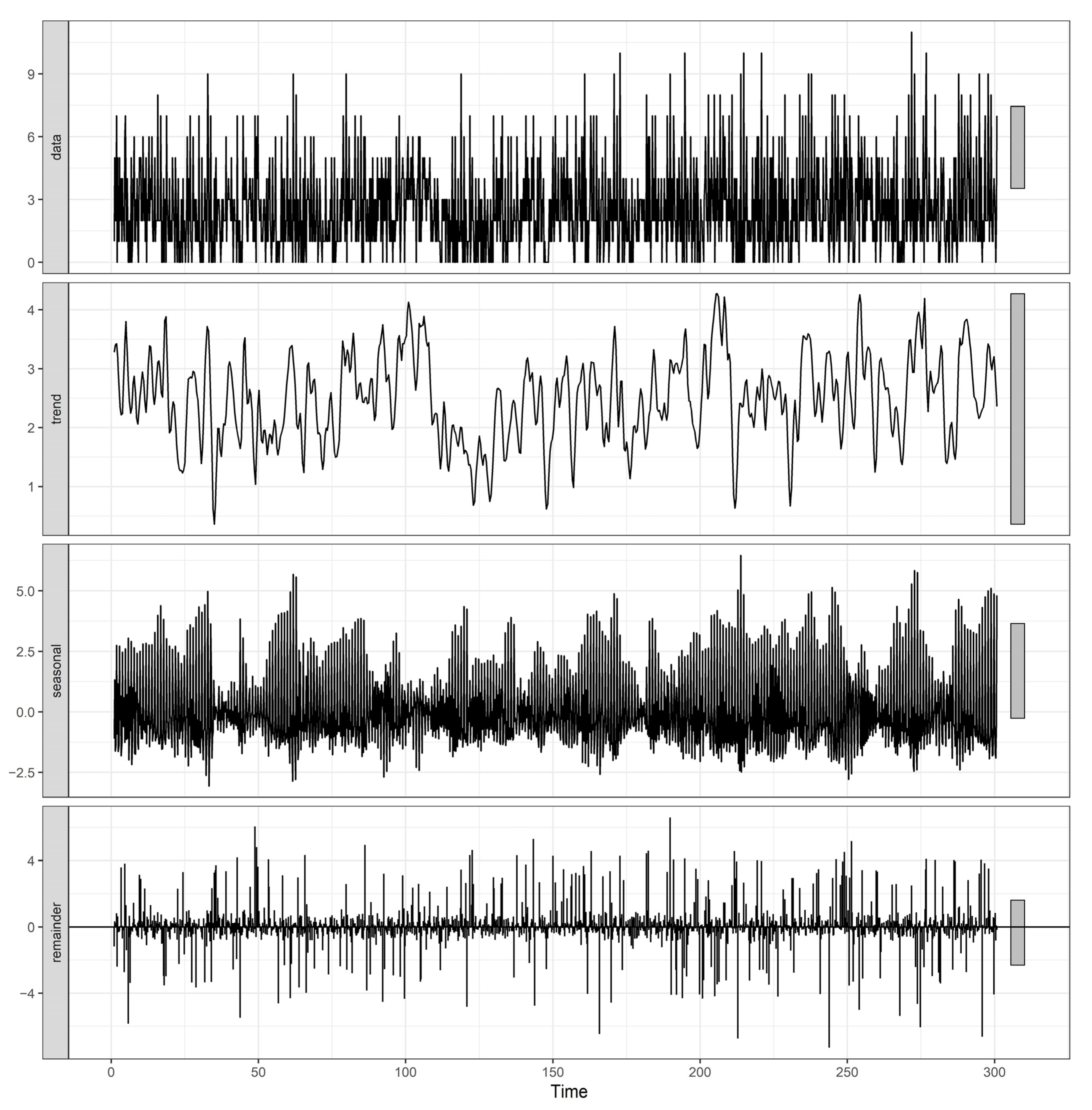
In this study, we considered five surgical units and their demands. In each time-series, there are two major components—namely, seasonality and trends—which play major roles in predictions. The seasonal and trend decomposition using loess (STL) is the best method for understanding seasonality and trend within a time-series [34]. Figure 3 shows the “STL” plot for the GA surgical unit. The data plotted in the first (top) panel are the daily surgical demand for the GA surgical unit. The second panel represents the trend component, which shows low frequency variation in the data along with non-stationary, long-term changes in the level. This is followed by the seasonal component in the third panel, which presents variation in the data at or near the seasonal frequency. The fourth (bottom) panel presents the remainder component, which is the remaining variation in data beyond that in the trend and seasonal component. This process was completed for each surgical unit for the entire data, showing that the data were composed of both seasonality and trends.

3.1. Model Results

In this study, 16 models (four simple models and 12 hybrid models) were developed, and the performances of these models were compared to identify the best-performing model for each surgical unit. A comparison of the consolidated results of all these models is presented in Table 3.
The baseline model was built for benchmarking and comparisons with the results of other models. This model predicted the demand for the KA surgical unit much better than other surgical units. Among these, the prediction was poor for the GA surgical unit, for which the error rates were three times more than those of the KA surgical unit.
With respect to the SARIMA model, the main requirement for its implementation is a stationary time-series. The augmented Dickey–Fuller (ADF) test was conducted using the “adf.test” function, which showed that the time-series of each surgical unit was stationary. To identify the optimal SARIMA model for each surgical unit, the “auto.arima” function was used and the model with the lowest Akaike’s information criterion (AIC) value was selected. As each surgical unit featured seasonality and trends, each unit was assigned a unique SARIMA model. For each of the SARIMA models, the residuals, their corresponding autocorrelation functions (ACFs), and histograms were plotted; the plots for the GA surgical unit are presented in Figure 4. As with the baseline model, the SARIMA model also performed better for the KA surgical unit and worse for the GA surgical unit.
With regard to the SVR model, in the model-building phase, the “eps-regression” type was used for predicting the demand in each surgical unit. The BA surgical unit demonstrated a lower RMSE, but higher MAE, compared with the EN surgical unit. This means that the EN surgical unit displayed a larger error in some cases but a smaller error in many cases, as compared with the BA surgical unit. As with the baseline and SARIMA models, the KA surgical unit had the lowest MAE and the GA surgical unit had the highest MAE, compared with all the other surgical units. Additionally, the baseline model performed better than the simple SVR model.
The forecasts from the MLP model showed that the KA surgical unit displayed marginally higher error values than the SARIMA model. All the surgical units demonstrated smaller error values than the baseline model. The BA surgical unit showed the best performance under this model, compared with the baseline and SVR models.
The LSTM model forecasted that the KA surgical unit would also demonstrate better results, compared with the other surgical units. The KA surgical unit showed the best performance under this model, compared with the baseline, SARIMA, and SVR models. The BA surgical unit had marginally higher error values than the SARIMA model. The results showed that the deep learning model does not always provide better results.
With respect to the SARIMA–SVR model, for each of the surgical units, the parameters from the best-performing simple SARIMA model were used to predict the initial values, and their corresponding residuals were predicted using an SVR model with the same parameters as the simple SVR model. The predicted results were added together, in order to make the final demand prediction. The comparison of the results showed that the simple SARIMA model performed better than the SARIMA–SVR hybrid model. For example, consider the GA surgical unit in which the simple SARIMA model outperformed the hybrid SARIMA–SVR model. Figure 5 presents the actual vs. forecast values for SARIMA and SARIMA–SVR models, respectively. Here, the hybrid model created more and larger errors when compared with the simple SARIMA–SVR model.
The SAIMA–SVR model was built for each surgical unit in which the simple SVR model was used to predict the initial results, and the residual values from this model were predicted using the SARIMA model. In terms of the SVR–SARIMA model, the error rates were higher when compared with the SARIMA–SVR model for EN, KA and BA surgical units. In comparison within the surgical units, this model performed well for the KA surgical unit. The model did not perform well for GA, UR and BA surgical units when compared with the simple SVR model.
The SARIMA–MLP model was similar to the SARIMA–SVR model but, here, the MLP model was used instead of the SVR to predict the demand. A comparison of the results showed that the hybrid model performed better than the simple MLP model, but not as well as the simple SARIMA model. As with all the other cases, the KA unit featured the best results, compared to all the other surgical units.
The MLP–SARIMA model was similar to the SVR–SARIMA model but, here, the MLP model was used instead of the SVR to predict the demand. The performance of this model was not as effective as that of the SARIMA–MLP model except for the KA surgical unit. As with the SARIMA–MLP model, the KA surgical unit obtained the best results, compared to all the other surgical units.
The SARIMA–LSTM model was similar to the SARIMA–SVR model but, here, the LSTM model was used to predict the demand, instead of the SVR. The simple SARIMA model provided better results, as compared with this hybrid model, for the BA surgical unit.
The LSTM–SARIMA model was similar to the SVR–SARIMA model but, here, the LSTM model was used instead of the SVR model to predict the demand. The performance was similar to that of the SARIMA–LSTM model, but the LSTM–SARIMA model was not as effective as this SARIMA–LSTM model for KA and UR surgical units. The LSTM–SARIMA model had marginally higher error values for the BA surgical units when compared with the SARIMA–LSTM model.
The SVR–MLP model used the simple SVR model to predict the initial values, and the corresponding residuals were predicted using a simple MLP model. The predicted values were added together to make the final demand prediction. As with all the other model results presented so far, the KA surgical unit demonstrated the best performance results. In addition, compared with the results of all the models, none of the surgical units demonstrated better prediction results when using the SVR–MLP model when compared to all the other models presented above.
In the MLP–SVR model, the simple MLP model was used to predict the initial values and the corresponding residuals were predicted using the simple SVR model. This model performed poorly for forecasting the demand when compared with the SVR–MLP model, except for the GA and BA surgical units. As with all the other models, the MLP–SVR model was able to forecast the surgical demand of the KA surgical unit.
The SVR–LSTM model was similar to the SVR–MLP model but, here, the LSTM model was used to predict the demand instead of the MLP. In this model, the KA surgical unit also provided better performance results.
The LSTM–SVR model was similar to the MLP–SVR model, but, here, the LSTM model was used instead of the MLP model to predict the demand. The LSTM–SVR model performed poorly when compared to the SVR–LSTM model for the EN and GA surgical units.
The MLP–LSTM model used the simple MLP model to predict the initial values, while the corresponding residuals were predicted using the simple LSTM model. The predicted values were added together to make the final demand prediction. In this model, the KA surgical unit also offered better results; however, most of the other models outperformed this hybrid model.
The final hybrid model was the LSTM–MLP model. This hybrid model was similar to the LSTM–SVR model but, here, instead of the SVR model, the MLP model was used for forecasting the demand. According to our comparison, the LSTM–MLP model outperformed the MLP–LSTM model except for the KA and UR surgical unit. As with all the other models, the forecast of surgical demand for the KA surgical unit was better than that of the other surgical units.

3.2. Accuracy Comparison

To select the model, the performance values of all the models (see Table 3) were compared. A comparison of the models clearly showed that the simple SARIMA–MLP model provided the best performance for the EN surgical unit; for the KA surgical unit, the SVR–LSTM provided the best performance; and, for the BA surgical unit, the LSTM–SARIMA hybrid model provided the best performance.
The remaining surgical units were the GA and UR units. For the GA unit, the simple LSTM model provided the lowest MAE and the SARIMA–LSTM model provided the lowest RMSE. For the UR surgical unit, the SARIMA–LSTM model provided the lowest MAE and the LSTM–SARIMA provided the lowest RMSE. As the preferred performance parameter was MAE, the simple LSTM model was preferred for the GA surgical unit and the SARIMA–LSTM hybrid model was the preferred model for the UR surgical unit.

4. Discussion

In this study, four simple models and twelve hybrid models were studied for five surgical units. The results indicated that the surgical unit GA had the best prediction results when using the simple LSTM model, surgical unit EN had the best prediction results when using the SARIMA–MLP model, two surgical units—UR and KA—had the best prediction results using the SARIMA–LSTM hybrid model, and surgical unit BA had the best prediction results when using the LSTM–SARIMA model. This shows that there is no universal model that can provide the best predictions for all surgical units. Therefore, hospitals need to use different models for each surgical unit in order to predict their demand.
The SARIMA–LSTM model predicted the demand more effectively for the UR surgical unit, which featured the highest number of elective surgeries. This hybrid model was able to decrease the errors by 18%. According to the results, the simple SARIMA model was able to decrease the MAE by 15%, while 3% of the improvement was due to the LSTM model.
The LSTM–SARIMA model predicted the demand more effectively for the BA surgical unit. This unit featured only half the number of elective surgeries and almost the same number of emergency surgeries as the UR surgical unit. Here, both the simple SARIMA and simple LSTM model had similar error rates in which the models were able to decrease the MAE by 26% when compared with the baseline model. Whereas the LSTM–SARIMA model was able to decrease the MAE by 31% when compared with the baseline model.
Nearly one third of the surgeries performed by the KA surgical unit are emergency surgeries. Therefore, an accurate demand prediction for this unit is important. All the models were more effective than baseline at predicting demand in the KA surgical unit. Except for the simple SVR model and hybrid models with SVR model, every other model was able to reduce the MAE by more than 40%; however, among all the models, the SARIMA–LSTM hybrid model demonstrated the lowest MAE values, with a 45% reduction compared with the baseline.
In contrast to the work of Taskaya-Temizel and Casey [25], this study showed that at least one hybrid model outperformed the simple SARIMA model for all surgical units. Figure 6 presents the actual vs. SARIMA and actual vs. SARIMA–LSTM forecasted surgical demand values for the GA surgical unit. The difference between the performance of these model is not easily identifiable from this Figure 6 because the hybrid SARIMA–LSTM outperformed the simple SARIMA model by reducing the MAE by nearly 1%.
The SVR–SARIMA, MLP–SARIMA, and LSTM–SARIMA models performed poorly when compared with the SARIMA–SVR, SARIMA–MLP, and SARIMA–LSTM, respectively. These performances were expected because the initial non-linear models were able to forecast both the linear and non-linear components of the time-series data, whereas the SARIMA model was not able to forecast the random error values and the residuals from the initial non-linear model. Therefore, when building a hybrid model with a linear model and a non-linear model, it is more effective to build the linear model and then use the non-linear model to forecast the residuals and the random error in the time-series.
However, there were some limitations to this study. First, only in-patient surgeries were studied, and not the demand for day surgeries. As some of the surgical units performed quite a substantial number of day surgeries each day, this might have had an impact on the surgeries’ resource allocations. Second, only 16 different models were explored for this study. Finally, the selected models should be updated periodically, in order to improve the accuracy of the demand prediction.

5. Conclusions

In this study, we found that hybrid modeling performed more effectively for most cases and the single LSTM model performed better in one case for the demand prediction of in-patient dayshift surgeries in a Norwegian hospital. The results showed that there is a need to have unique models for demand prediction in each surgical unit of a hospital, as each unit has unique demand patterns. With the predicted demand values, each surgical unit can predict the demand values in advance, thus ensuring better resource allocation. Future studies should focus on eliminating the limitations presented in the Discussion section.

Funding

This research received no external funding.

Institutional Review Board Statement

Not applicable.

Informed Consent Statement

Not applicable.

Data Availability Statement

Not applicable.

Acknowledgments

The author would like to thank Berit Irene Helgheim, Faculty of Logistics, Molde University College—Specialized University in Logistics for the valuable advice and guidance with this study.

Conflicts of Interest

The author declares no conflict of interest.

References

  1. Taylor, R.A.; Pare, J.R.; Venkatesh, A.K.; Mowafi, H.; Melnick, E.R.; Fleischman, W.; Hall, M.K. Prediction of In-hospital Mortality in Emergency Department Patients With Sepsis: A Local Big Data-Driven, Machine Learning Approach. Acad. Emerg. Med. 2016, 23, 269–278. [Google Scholar] [CrossRef] [Green Version]
  2. Perng, J.W.; Kao, I.H.; Kung, C.T.; Hung, S.C.; Lai, Y.H.; Su, C.M. Mortality Prediction of Septic Patients in the Emergency Department Based on Machine Learning. J. Clin. Med. 2019, 8, 1906. [Google Scholar] [CrossRef] [Green Version]
  3. Raita, Y.; Goto, T.; Faridi, M.K.; Brown, D.F.M.; Camargo, C.A., Jr.; Hasegawa, K. Emergency department triage prediction of clinical outcomes using machine learning models. Crit. Care 2019, 23, 64. [Google Scholar] [CrossRef] [Green Version]
  4. Lucini, F.R.; Reis, M.A.d.; Silveira, G.J.C.d.; Fogliatto, F.S.; Anzanello, M.J.; Andrioli, G.G.; Nicolaidis, R.; Beltrame, R.C.F.; Neyeloff, J.L.; Schaan, B.D.A. Man vs. machine: Predicting hospital bed demand from an emergency department. PLoS ONE 2020, 15, e0237937. [Google Scholar] [CrossRef]
  5. Lin, A.X.; Ho, A.F.W.; Cheong, K.H.; Li, Z.; Cai, W.; Chee, M.L.; Ng, Y.Y.; Xiao, X.; Ong, M.E.H. Leveraging Machine Learning Techniques and Engineering of Multi-Nature Features for National Daily Regional Ambulance Demand Prediction. Int. J. Environ. Res. Public Health 2020, 17, 4179. [Google Scholar] [CrossRef] [PubMed]
  6. Chen, A.Y.; Lu, T.-Y. A GIS-Based Demand Forecast Using Machine Learning for Emergency Medical Services. In Computing in Civil and Building Engineering (2014); American Society of Civil Engineers: Orlando, FL, USA, 2014; pp. 1634–1641. [Google Scholar]
  7. Chan, E.W.; Taylor, S.E.; Marriott, J.; Barger, B. An intervention to encourage ambulance paramedics to bring patients’ own medications to the ED: Impact on medications brought in and prescribing errors. Emerg. Med. Australas 2010, 22, 151–158. [Google Scholar] [CrossRef] [PubMed]
  8. Ekström, A.; Kurland, L.; Farrokhnia, N.; Castrén, M.; Nordberg, M. Forecasting emergency department visits using internet data. Ann. Emerg. Med. 2015, 65, 436–442.e431. [Google Scholar] [CrossRef] [PubMed] [Green Version]
  9. Farmer, R.D.; Emami, J. Models for forecasting hospital bed requirements in the acute sector. J. Epidemiol. Community Health 1990, 44, 307–312. [Google Scholar] [CrossRef] [Green Version]
  10. Jones, S.A.; Joy, M.P.; Pearson, J. Forecasting demand of emergency care. Health Care Manag. Sci. 2002, 5, 297–305. [Google Scholar] [CrossRef] [PubMed] [Green Version]
  11. Schweigler, L.M.; Desmond, J.S.; McCarthy, M.L.; Bukowski, K.J.; Ionides, E.L.; Younger, J.G. Forecasting models of emergency department crowding. Acad. Emerg. Med. 2009, 16, 301–308. [Google Scholar] [CrossRef] [PubMed]
  12. Zhou, L.; Zhao, P.; Wu, D.; Cheng, C.; Huang, H. Time series model for forecasting the number of new admission inpatients. BMC Med. Inform. Decis. Mak. 2018, 18, 1–11. [Google Scholar] [CrossRef] [Green Version]
  13. Zinouri, N.; Taaffe, K.M.; Neyens, D.M. Modelling and forecasting daily surgical case volume using time series analysis. Health Syst. 2018, 7, 111–119. [Google Scholar] [CrossRef] [PubMed]
  14. Purwanto; Eswaran, C.; Logeswaran, R. An enhanced hybrid method for time series prediction using linear and neural network models. Appl. Intell. 2012, 37, 511–519. [Google Scholar] [CrossRef]
  15. Yolcu, U.; Egrioglu, E.; Aladag, C.H. A new linear & nonlinear artificial neural network model for time series forecasting. Decis. Support Syst. 2013, 54, 1340–1347. [Google Scholar] [CrossRef]
  16. Gupta, D.; Pratama, M.; Ma, Z.; Li, J.; Prasad, M. Financial time series forecasting using twin support vector regression. PLoS ONE 2019, 14, e0211402. [Google Scholar] [CrossRef] [PubMed]
  17. Tsai, M.-C.; Cheng, C.-H.; Tsai, M.-I.; Shiu, H.-Y. Forecasting leading industry stock prices based on a hybrid time-series forecast model. PLoS ONE 2019, 13, e0209922. [Google Scholar] [CrossRef] [Green Version]
  18. Zhang, G.P. Time series forecasting using a hybrid ARIMA and neural network model. Neurocomputing 2003, 50, 159–175. [Google Scholar] [CrossRef]
  19. Golmohammadi, D. Predicting hospital admissions to reduce emergency department boarding. Int. J. Prod. Econ. 2016, 182, 535–544. [Google Scholar] [CrossRef]
  20. Guo, Y.; Feng, Y.; Qu, F.; Zhang, L.; Yan, B.; Lv, J. Prediction of hepatitis E using machine learning models. PLoS ONE 2020, 15, e0237750. [Google Scholar] [CrossRef]
  21. Volkova, S.; Ayton, E.; Porterfield, K.; Corley, C.D. Forecasting influenza-like illness dynamics for military populations using neural networks and social media. PLoS ONE 2017, 12, e0188941. [Google Scholar] [CrossRef] [Green Version]
  22. Zou, J.-J.; Jiang, G.-F.; Xie, X.-X.; Huang, J.; Yang, X.-B. Application of a combined model with seasonal autoregressive integrated moving average and support vector regression in forecasting hand-foot-mouth disease incidence in Wuhan, China. Medicine 2019, 98, e14195. [Google Scholar] [CrossRef]
  23. Wang, H.; Tian, C.W.; Wang, W.M.; Luo, X.M. Time-series analysis of tuberculosis from 2005 to 2017 in China. Epidemiol. Infect. 2018, 146, 935–939. [Google Scholar] [CrossRef] [Green Version]
  24. Wang, Y.-w.; Shen, Z.-z.; Jiang, Y. Comparison of autoregressive integrated moving average model and generalised regression neural network model for prediction of haemorrhagic fever with renal syndrome in China: A time-series study. BMJ Open 2019, 9, e025773. [Google Scholar] [CrossRef] [Green Version]
  25. Taskaya-Temizel, T.; Casey, M.C. A comparative study of autoregressive neural network hybrids. Neural Netw. 2005, 18, 781–789. [Google Scholar] [CrossRef] [Green Version]
  26. Boyle, J.; Jessup, M.; Crilly, J.; Green, D.; Lind, J.; Wallis, M.; Miller, P.; Fitzgerald, G. Predicting emergency department admissions. Emerg. Med. J. 2012, 29, 358. [Google Scholar] [CrossRef] [PubMed] [Green Version]
  27. Litvak, E.; Long, M.C. Cost and quality under managed care: Irreconcilable differences. Am. J. Manag. Care 2000, 6, 305–312. [Google Scholar] [PubMed]
  28. Tiwari, V.; Furman, W.R.; Sandberg, W.S. Predicting Case Volume from the Accumulating Elective Operating Room Schedule Facilitates Staffing Improvements. Anesthesiology 2014, 121, 171–183. [Google Scholar] [CrossRef] [PubMed] [Green Version]
  29. Syntetos, A.A.; Boylan, J.E.; Croston, J.D. On the categorization of demand patterns. J. Oper. Res. Soc. 2005, 56, 495–503. [Google Scholar] [CrossRef]
  30. Hyndman, R.J.; Athanasopoulos, G. Forecasting: Principles and Practice, 3rd ed.; OTexts: Melbourne, VIC, Australia, 2021. [Google Scholar]
  31. Hyndman, R.J.; Khandakar, Y. Automatic Time Series Forecasting: The forecast Package for R. J. Stat. Softw. 2008, 27, 22. [Google Scholar] [CrossRef] [Green Version]
  32. Chollet, F.; Allaire, J.J. Deep Learning with R; Manning Publications: Shelter Island, NY, USA, 2018; p. 360. [Google Scholar]
  33. Yu, G.; Feng, H.; Feng, S.; Zhao, J.; Xu, J. Structure of the SARIMA–NNAR combined model. PLoS ONE 2021. [Google Scholar] [CrossRef]
  34. Cleveland, R.B.; Cleveland, W.S.; McRae, J.E.; Terpenning, I. STL: A seasonal-trend decomposition. J. Off. Stat. 1990, 6, 3–73. [Google Scholar]
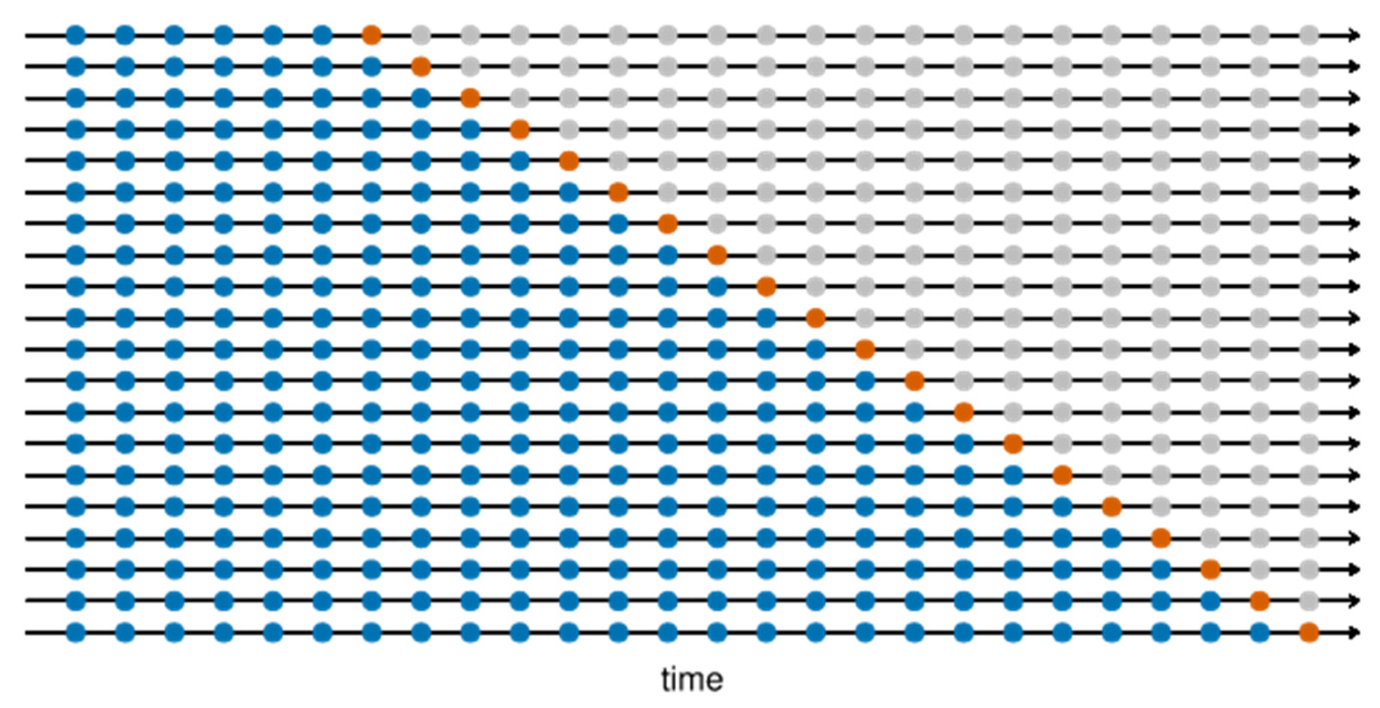
Figure 1. Cross-validation on a rolling basis of the time-series data [30].
Ai 02 00032 g001
Figure 2. Structure of the hybrid model [33].
Ai 02 00032 g002
Figure 3. Time-series plot of the GA surgical unit.
Ai 02 00032 g003
Figure 4. (a) Plot of the residuals, (b) ACF plot of the residuals, and (c) histogram of the residuals from the SARIMA model for the GA surgical unit.
Ai 02 00032 g004
Figure 5. (a) Actual vs. SARIMA forecast and (b) actual vs. SARIMA–SVR forecast for the GA surgical unit.
Ai 02 00032 g005
Figure 6. Plot of (a) actual vs. SARIMA and (b) actual vs. SARIMA–LSTM forecasted surgical demand values for the GA surgical unit.
Ai 02 00032 g006
Table 1. Daily percentage share of surgeries by each surgical unit.
Surgical
Units
Percentage Share of Surgeries (%)
MondayTuesdayWednesdayThursdayFridayOverall
EN0.77%3.49%1.02%2.87%1.60%9.75%
GA3.52%4.24%3.96%3.84%12.10%27.65%
KA0.51%1.66%0.73%0.74%0.52%4.16%
UR9.77%3.53%13.81%4.22%4.99%36.31%
BA3.64%3.53%2.69%6.77%5.49%22.13%
Total18.21%16.45%22.21%18.44%24.70%100.00%
Table 2. Total number of records during the period 2012–2018.
Surgical
Units
Elective
Patients
Emergency
Patients
Total
Patients
% of Emergency
Patients
EN17056517703.67%
GA37931225501824.41%
KA51024575532.45%
UR623235865905.43%
BA363937740169.39%
Total15,879227018,14912.51%
Table 3. Prediction performance results of the ten models for each surgical unit.
ModelsENGAKAURBA
MAERMSEMAERMSEMAERMSEMAERMSEMAERMSE
Baseline0.6770.9711.7602.3940.5430.8661.1731.5851.1971.607
SARIMA0.5870.8941.3931.7870.3230.6610.9971.2900.8801.208
SVR1.3402.7592.5803.7720.8801.9392.1403.6321.4172.410
MLP0.6130.8521.6202.2540.3270.6631.0901.4110.9131.238
LSTM0.6700.9981.3471.8060.3030.6461.0301.3600.8901.218
SARIMA–SVR0.7301.1933.0635.7490.6131.3172.9277.0461.6402.725
SVR–SARIMA0.9801.7012.7034.6570.8632.0032.6574.9781.8603.733
SARIMA–MLP0.5170.8101.4131.8000.3430.6611.0071.3320.8731.197
MLP–SARIMA0.5970.8891.6732.2050.3230.6461.0401.3470.8801.200
SARIMA–LSTM0.6630.9951.3801.7800.3000.6430.9631.2950.8831.221
LSTM–SARIMA0.5830.8961.3601.7910.3100.6510.9801.2880.8271.134
SVR–MLP0.8831.4323.0376.2110.7071.5542.0132.9202.0773.894
MLP–SVR1.1802.3712.7034.2340.8371.8252.4104.2671.8633.349
SVR–LSTM1.0831.8572.3533.8041.1102.9372.1533.5031.8673.271
LSTM–SVR1.1073.4742.6704.6840.7371.7311.9572.8541.7233.015
MLP–LSTM0.6370.9641.5872.1170.3030.6461.0001.3060.9731.349
LSTM–MLP0.6330.8761.4771.9720.3330.6631.0101.3100.8871.200
Publisher’s Note: MDPI stays neutral with regard to jurisdictional claims in published maps and institutional affiliations.