Abstract
Defect detection in images is a challenging task due to the existence of tiny and noisy patterns on surface images. To tackle this challenge, a defect detection approach is proposed in this paper using statistical data fusion. First, the proposed approach breaks a large image that contains multiple separate defects into smaller overlapping patches to detect the existence of defects in each patch, using the conventional convolutional neural network approach. Then, a statistical data fusion approach is proposed to maintain the spatial coherence of cracks in the image and aggregate the information extracted from overlapping patches to enhance the overall performance and robustness of the system. The proposed approach is evaluated using three benchmark datasets to demonstrate its superior performance in terms of both individual patch inspection and the whole image inspection.
1. Introduction
Defect inspection using computer vision technology is an important task in various industries [1,2,3,4], including railroad defects on steel surfaces [5], concrete cracks [6], tunnel inspection [7].
Various visual inspection methods have been developed in the literature for automatic defect detection in the image. These methods can be classified into two categories, including defect classification and defect localization in the image. The former defect classification approach [1] essentially addresses the problem of pixel classification, where the goal is to classify each image pixel as a Defect or Non-Defect. The latter defect location approach [2] aims to place a tight-fitting boundary around each defect in the image.
The capability of visual inspection methods relies on how to acquire defect features in an automated and effective manner. The existing visual inspection methods can be classified into categories: (1) traditional approaches; (2) statistical-based approaches; (3) learning-based approaches. First, the traditional defect detection methods include edge detection, morphological operations for strong edges and less noisy patterns. These methods model the texture primitives and displacements for repetitive patterns such as textile and fabrics. The statistical distributions of pixel values are studied in more complicated image analysis techniques, such as crack blob features [8], Gabor features [9], and wavelet features [10]. Second, statistical approaches are usually used to detect defects of flat steel surface by evaluating the regular distribution of pixel intensities. A low-rank representation based on texture prior for detection of defects on natural surfaces is developed in [11]. Third, deep learning technology, such as ResNet [12], YOLO [13], Mask R-CNN [14], has the potentials to address this issue in representation learning by building complex features. A convolutional neural network is proposed in [15] to detect road cracks. Several convolutional neural network architectures are evaluated for defect localization [16]. A multiple feature learning approach is proposed in [17]. The classification results of several convolutional neural networks are fused to determine whether it is false positive or not [18]. Various image fusion methods have also been developed in [19,20,21] to combine multiple images with various qualities for image enhancement. A video-based inspection method is proposed in [22] by applying Bayesian fusion on classification results of continuous frames. An automatic surface inspector by extracting transferred features of an image from a pre-trained model and generating defect heat map on the extracted transferred feature to identify defect areas in [23].
The major challenge of defect detection in images is the existence of tiny cracks and noisy patterns on metallic surfaces. Figure 1 illustrates tiny defects in the image, where some defects are surrounded by noisy patterns while some are hardly visible in low contrast image. Furthermore, defect could be connected or isolated in an image. For images that consist of multiple separate defects, it may be insufficient to identify the separate defects using the single image classifiers mentioned in the previous paragraph.
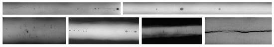
Figure 1.
Examples of defects in images. The challenge of defect detection in images is the existence of tiny cracks and noisy patterns in images.
To tackle this challenge, a defect detection approach is proposed in this paper. The proposed approach breaks a large image that contains multiple defects into smaller overlapping patches to detect the existence of defect in each patch, by training a convolutional neural network (CNN) patch classifier. The overlapped regions can then be fused by Bayes theorem to determine whether they are classified as defects or not. By breaking the image into small patches, each patch is responsible for a smaller number of defects and the defect detection task could be potentially easier.
The rest of this paper is organized as follows. Section 2 highlights the challenges of existing approaches that motivates the proposed approach, as well as the novelty and experimental design of the proposed approach. Section 3 presents the proposed defect detection framework. Section 4 presents the extensive performance evaluation of the proposed approach using three benchmark datasets and discusses the results. Finally, Section 5 concludes this paper.
2. Motivation
This section summarizes the challenges of existing approaches, the novelty and experimental design of the proposed approach as follows.
Challenges of existing approaches: To tackle tiny defects in the image as illustrated in Figure 1, the current state-of-the-art methods usually apply two key strategies [1,2]: global-based methods, and local-based methods. The global-based methods exploits features (either hand-crafted features or deeply learned features) extracted from the whole image to make binary decision whether the input image is defect or not. These features extracted from the whole image are usually insufficient to identify the separate defects. On the other hand, the local-based methods exploits local features learned from the deeply learned feature map to localize a tight-fitting boundary around each defect in the image. These methods require complicated data labelling (either region-based labelling or pixel-based labelling) for model training.
Motivation of novelty of the proposed approach: To benefit deeply learned features from images (in global-based methods) and avoid complicated data labelling (in local-based methods), a two-stage defect detection approach is proposed in this paper. The key characteristics of this paper are summarized as follows.
- The gist of the proposed approach is to break a large image that contains multiple separate defects into small overlapping patches to detect the existence of defect in each patch using the convolutional neural network classifier, and then re-combines the patches back to form the final defect decision using a statistical data fusion approach.
- The proposed approach requires less defect labelling efforts in the model training, since it only needs patch-based labelling. This contrasts with that the region-based labelling (for defect object detection) or pixel-based labelling (for defect region segmentation) are required in the literature.
Design of experiments: The proposed approach is evaluated using three publicly available benchmark datasets [24,25,26] for performance evaluation. Furthermore, for each dataset, two kinds of experiments are conducted, including (1) classifying individual patch, and (2) detecting defect regions in the whole image. These two experiments are used to justify the performance of two components (individual patch classifier and the decision fusion) of the proposed approach.
3. Proposed Defect Detection Approach
The rationale of the proposed approach is to break a large image that contains multiple defects into overlapping patches so that each small region could be determined as Defect or not. To be more specific, the proposed approach consists of two key components. First, the conventional convolutional neural network method is exploited to detect overlapping patches in the image. Second, a Bayesian data fusion approach is proposed to aggregate the information extracted from overlapping patches to enhance the overall performance and robustness of the system. These two components are described in the following sections in detail.
3.1. Patch Classifier
The first component of the proposed approach is to develop a patch classifier to decide whether each overlapping patch is a Defect patch or Non-Defect patch. For that, a patch extractor is first built to extract patches from the training image dataset and to label each of them as Defect or Non-Defect based on the corresponding ground truth patch. For each image dataset, patches are extracted with a stride size of , which means each patch overlaps a neighboring patch by . Each patch is also labelled as Defect or Non-Defect, depending on the number of positive defect pixels in the corresponding ground truth patch. If the corresponding ground truth patch contains positive pixels, the patch is labelled as Defect, or Non-Defect if otherwise. An example of the extracted patches is shown in Figure 2.
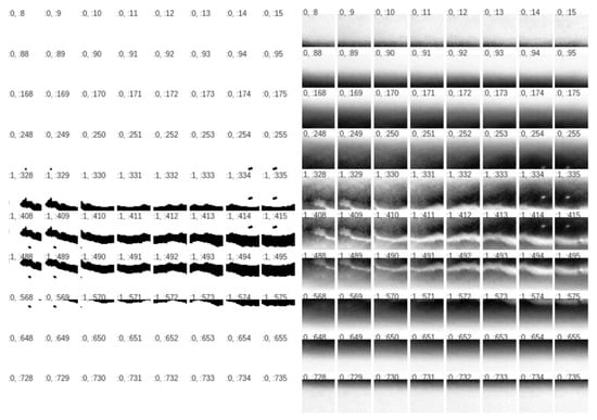
Figure 2.
Examples of ground truths (left) and extracted patches (right), which are denoted as Class:PatchIndex.
The proposed patch classifier is illustrated in Figure 3. It consists of the conventional -16 network backbone [27], as illustrated in Figure 4, to extract features and an additional two-layer multi-layer feed forward (MLFF) head to do binary classification. The two additional layers consist of the following in sequence: linear layer of 20 nodes; relu; batch normalization; dropout (); linear layer of 20 nodes; batch normalization; single output node with Sigmoid activation. The training image data set is thus fed to the patch classifier and trained features are extracted and then flattened and put through two dense layers and a Sigmoid activation function of the binary classification exercise. The cross-entropy loss function (denoted as L) is used in the proposed approach as
where is an averaging function over all patches, is the label class of n-th patch, is the prediction of n-th patch, and and are the weights assigned to class 1 (Defect) and class 0 (Non-Defect) respectively.
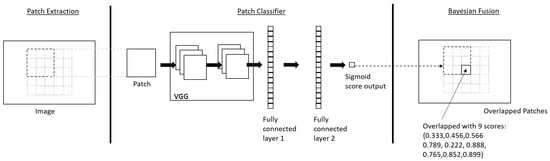
Figure 3.
The architecture of the proposed defect detection approach.
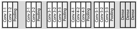
Figure 4.
The details of the VGG-16 backbone model [27] used in the proposed approach.
3.2. Bayesian Data Fusion of Overlapping Patch Classifiers
The patch classifier described in the previous section is applied on the image so that each overlapping region of the image will have multiple scores, which are obtained from the patch classifier, as illustrated in Figure 5. Given these multiple scores, a Bayesian data fusion approach is proposed in this section to obtain the single final probability of the patch being Defect or Non-Defect.
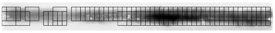
Figure 5.
An illustration of overlapping patches that are classified as defects. Each patch is highlighted using the black color rectangular bounding box.
First, the histogram and the probability density function (PDF) of the classifier scores are collected for the Non-Defect and the Defect classes from the training image datasets. Figure 6 shows the PDFs of and , where is the classification score of patch i and is the Defect class and is the Non-Defect class.
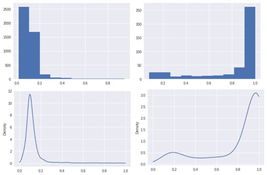
Figure 6.
Histograms (top) and PDFs (bottom) for Non-Defect class (left) and Defect class (right).
Then, the overlapping region is determined as Defect subject to the following condition
where controls the sensitivity of decision making, and is the classification score for the overlapping patch over the same region. Taking Log function on both sides of (2) we have
which can be further rewritten as
which can be simplified as
where i is the number of overlapping patch in a region, and are likelihood functions, is the prediction of the i-th overlapping patch, is Defect and is Non-Defect. and can be ignored since contains them. The region will be determined as Defect if the left-hand side of (5) is bigger than ; otherwise, it is determined as Non-Defect. The PDFs of the Defect and the Non-Defect Classes are estimated using non-parametric kernel density estimation (KDE) method.
Finally, after each region is determined as Defect or Non-Defect, an external bounding box is applied to contain the connected defect regions. An example is shown in Figure 7.
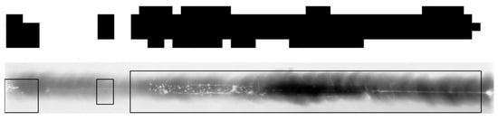
Figure 7.
The detected defect regions, which are illustrated as black regions in the binary image (top photo) and illustrated using the bounding boxes and overlaid on the original image (bottom photo).
To summarize, the PDF of the scores given Defect class and the PDF of the scores given Non-Defect class are collected from the training image dataset. A test image is also extracted into patches and each test image patch is incorporated into the trained patch classifier. The test image patches are then overlayed in the original spatial arrangements and each overlapped region will have multiple scores. Given the scores of each region, the probability of being Defect or Non-Defect could be established using Naive Bayes Theorem [22]. As such, each overlapping region could be determined as Defect or Non-Defect if the probability of being Defect is greater than the probability of being Non-Defect by a user-controlled threshold. Lastly, bounding boxes are used to contain the connected defect regions.
4. Experimental Results
4.1. Experimental Setup and Implementation Details
Three publicly available benchmark datasets are used in this paper for performance evaluation.
- The dataset I is the GDXray dataset [24]. It consists of 10 radiography images of metal pipes. Each image is approximately in resolution and is provided with pixel-wise ground truth. The first 5 images are used as training images and the last 5 images are used as the testing images.
- The dataset II is the Type-I RSDDs data set [25] that contains 67 express rails defect images. Each image is in resolution and is provided with pixel-wise ground truth. 47 images are randomly chosen as training images and the left-over 20 images are used as testing images.
- The dataset III is the NEU steel surface defect dataset [26] that consists of scratch defects from hot-rolled steel strip. There are 300 images in this dataset, each image has a resolution of pixels, with the coordinates of the ground truth bounding boxes provided. The area of ground truth bounding boxes are taken as the pixel-wise ground truth for this dataset. 200 images are randomly chosen as training images and the left-over 100 images are used testing images.
For each dataset, two kinds of experiments are conducted, including (i) classifying individual patch, and (ii) detecting defect regions in the whole image. For the first experiment, various defect patch classification approaches are evaluated in terms of accuracy and Receiver operating characteristic (ROC) curve. For the second experiment, ground truth bounding boxes are generated by first applying a Gaussian filter and then a connected-components algorithm on each pixel-wise ground truth to find connected components. Ground truth bounding boxes are put on top of the connected components by finding the maximum x, y and minimum x, y coordinates of each connected component. The areas of bounded ground truth regions are then compared with the areas of the final predicted bounding boxes results to obtain pixel-wise accuracy, mean Intersection Over Union (IOU), sensitivity, specificity, and precision. For each dataset, the proposed approach is only compared with the state-of-the-art deep learning-based approach for a fair performance evaluation. The stochastic gradient descent (SGD) is used to optimize the patch classifiers networks at a learning rate of . The threshold parameter for the binarization of Defect pixels and Non-Defect pixels used is percentile of the Bayesian fused scores.
4.2. Experimental Results
4.2.1. Dataset I: GDXray Dataset
Defect patch classification: The patch size used to extract the patches is . The proposed patch classifier is trained on 1405 Defect patches and 5445 Non-Defect patches, and is validated on 624 unseen Defect patches and 2312 unseen Non-Defect patches. The proposed patch classifier has achieved an accuracy of and an area under ROC curve of , which is higher than the benchmark reference [23]. The benchmark reference has used Decaf model for transfer learning and a patch size of instead. Figure 8 shows the histograms and PDFs of the classification scores from the validation set.
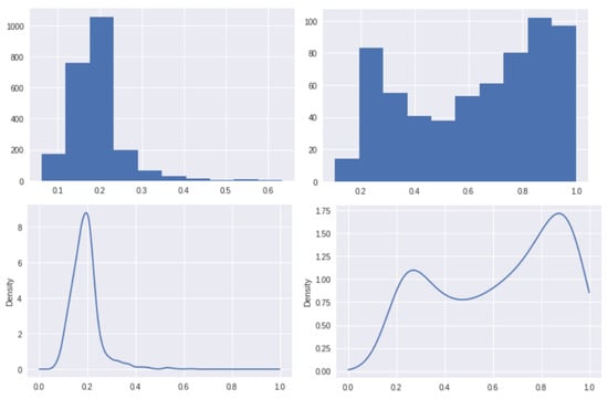
Figure 8.
The histograms (top row) and PDFs (bottom row) for Non-Defect class (left column) and Defect class (right column) of GDXray dataset [24].
Defect detection in the whole image:Table 1 and Table 2 show the accuracy, mean IOU and various scores of each test image. The results of all the five test images are shown in Figure 9.

Table 1.
The performance comparison (defect patch classifier) of various defect detection approaches using all three datasets. In this table, - indicates that there is no result available in the reference work.
Table 2.
The performance comparison (defect detection in whole image) of various defect detection approaches using all three datasets. In this table, - indicates that there is no result available in the reference work.
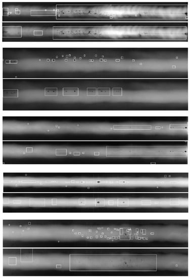
Figure 9.
Five pairs of defect detection results of the proposed approach (GDXray dataset [24]). Each pair of results consists of the ground truth bounding boxes (top) and detected bounding boxes (bottom).
Discussion: As seen from the results, the patch classifier could not differentiate some defect patches from Non-Defect patches as the defects are too small and similar in some images. A smaller patch size may have helped the patch classifier to achieve a better performance.
4.2.2. Dataset II: Type-I RSDDs Dataset
Defect patch classification: The patch size that is used to extract patches is . The proposed patch classifier is trained on 1098 Defect patches and 10523 Non-Defect patches, and is validated on 420 unseen Defect patches and 4561 unseen Non-Defect patches. The proposed patch classifier has reached an accuracy of and an area under ROC curve of . Table 1 and Table 2 show the comparison of the classification results. Figure 10 shows the histograms and PDFs of the classification scores from the validation set.
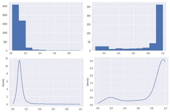
Figure 10.
The histograms (top row) and PDFs (bottom row) for Non-Defect class (left column) and Defect class (right column) of Type-I RSDDs data set [25].
Defect detection in the whole image:Table 1 and Table 2 show the overall accuracy, mean IOU and various scores of this dataset. The results of the sample test images are shown in Figure 11.
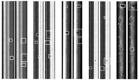
Figure 11.
Five pairs of defect detection results of the proposed approach (Type-I RSDDs data set [25]). Each pair of results consists of the ground truth bounding boxes (left) and detected bounding boxes (right).
Discussion: As seen from the results, the proposed model can detect all ground truths defect correctly. The proposed model also identified similar patterns as defects although they are not ground truths and are considered false positives.
4.2.3. Dataset III: NEU Steel Surface Defect Dataset
Defect patch classification: The patch size that is used for extraction is . The proposed patch classifier is trained on 5703 Defect patches and 8297 Non-Defect patches, and is validated on 3555 unseen Defect patches and 2445 unseen Non-Defect patches. The proposed patch classifier has achieved an accuracy of and an area under ROC curve of . Figure 12 presents the histograms and PDFs of the classification scores of the validation set.
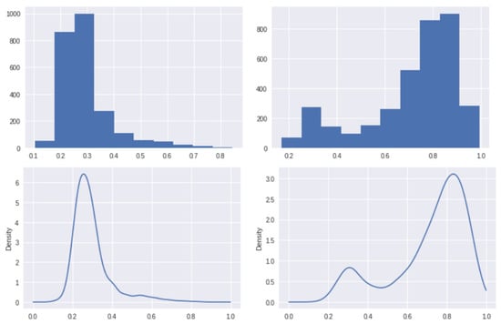
Figure 12.
The histograms (top row) and PDFs (bottom row) for Non-Defect class (left column) and Defect class (right column) of NEU steel surface defect dataset [26].
Defect detection in the whole image:Table 1 and Table 2 show the overall accuracy, mean IOU and various scores of this dataset. The results of sample test images are shown in Figure 13.
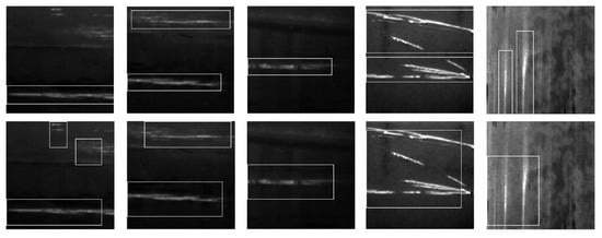
Figure 13.
Five pairs of defect detection results of the proposed approach (NEU steel surface defect dataset [26]). Each pair of results consists of the ground truth bounding boxes (top) and detected bounding boxes (bottom).
Discussion: As seen from the results, some defects are too close together and Bayesian fusion has fused separate defects together to form one bounding box that encompass the separate defects instead of bounding each defect separately. A smaller patch size may help the Bayesian fusion to separate the bounding boxes for defects that are close together.
4.3. Evaluation on Parameter Setting
Two key parameters of the proposed approach are the patch size and the threshold parameter (defined in (2)), which can affect the performance of the proposed approach. In view of this, the following two experiments have been conducted to evaluate the performance of the parameter setting of the proposed approach.
4.3.1. Patch Size of the Proposed Approach
First, the patch size can affect the performance of the patch classifier and the performance of the defect detection. Figure 14 shows the histograms and PDFs of the classification scores from the validation set of GDXray dataset [24] trained on patch size of 180. They are different from the results of patch size 120 shown in Figure 8. An experiment is conducted to evaluate the mean accuracy of defect detections on all five images of GDXray dataset [24] using patch sizes 180 and 120, respectively. Figure 15 shows difference in the final detection of defects in Image 2 of GDXray dataset [24]. A smaller patch size of 120 produces a much better result (mean accuracy score ) than using patch size 180 (mean accuracy score ).
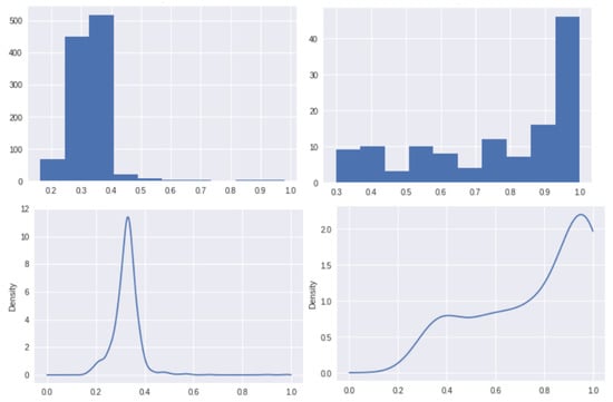
Figure 14.
Histograms (top) and PDFs (bottom) of the classification scores from the validation set of GDXray dataset [24] trained with a patch size of 180.

Figure 15.
The comparison of the proposed approach with different patch sizes 120 (top) and 180 (bottom) based on Image 2 of GDXray dataset [24].
4.3.2. Threshold Parameter of the Proposed Approach
The threshold parameter (defined in (2)) affects the binarization of Defect pixels and Non-Defect pixels after performing fusion of overlapped classification scores. A higher gets lesser defect pixels but makes it more precise. A lower gets more defect pixels but makes it less precise. Figure 16 shows results on Image 1 of GDXray dataset [24] by adjusting the threshold parameter to (top), (middle), and (bottom) percentile of the Bayes fused scores, respectively.
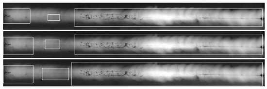
Figure 16.
The comparison of detected defects in Image 1 of GDXray dataset [24] by adjusting the threshold parameter (defined in (2)) to be (top row), (middle row), and (bottom row).
4.4. Evaluation on Computational Complexity
An experiment is conducted to evaluate the computational complexity (run-time) performance of the proposed approach, particularly in terms of the additional computational complexity introduced by the proposed statistical fusion module on the conventional deep learning-based framework. The proposed approach is implemented in a PC with CPU i7-8700K, 32GB RAM, GTX 2070Ti, Tensorflow 1.9. Two test images with different resolutions are used in this experiment, including (GDXray dataset [24]) and (Type-I RSDDs data set [25]. As seen from Table 3, the proposed approach indeed introduces additional complexity and takes more time in inference.
Table 3.
The run-time (seconds) performance of the proposed approach.
5. Conclusions
A defect detection in images approach has been proposed in this paper, by breaking a large image that contains multiple separate defects into small overlapping patches to detect the existence of defect in each patch using the convolutional neural network classifier, and then re-combines the patches back to form the final defect decision using a statistical data fusion approach. Compared with other detection or segmentation frameworks used in this research area, the proposed approach requires less defect labelling efforts in the model training, since it only needs patch-based labelling, not the region-based labelling (for defect object detection) or pixel-based labelling (for defect region segmentation). The proposed approach uses a fairly big box to cover small defects, it is less accurate compared with other segmentation framework that can provide accurate pixel-level defect labels.
The limitations of the proposed approach are acknowledged as follows. First, the proposed approach is more suitable to the defect datasets with noisy defect in images. In this scenario, some defects are surrounded by noisy patterns, while some are hardly visible in low contrast image. Second, the choice of the convolutional neural network backbone used in the proposed approach is not well justified, since we provide a flexible framework that can exploits the other types of recently developed convolutional neural network backbone instead of the -16 used in the current proposed approach. Third, it is interesting to study how to handle conflicting data to achieve more reliable decision fusion by combining decisions from individual patches [28,29].
Author Contributions
Conceptualization, Y.T.E.C., J.T.; Data curation, Y.T.E.C., J.T.; Formal analysis, Y.T.E.C., J.T.; Investigation, Y.T.E.C., J.T.; Methodology, Y.T.E.C., J.T.; Project administration, J.T.; Software, Y.T.E.C.; Supervision, J.T.; Validation, Y.T.E.C., J.T.; Visualization, Y.T.E.C., J.T.; Writing–original draft, Y.T.E.C., J.T.; Writing–review & editing, Y.T.E.C., J.T. All authors have read and agreed to the published version of the manuscript.
Funding
This research received no external funding.
Conflicts of Interest
The authors declare no conflict of interest.
References
- Luo, Q.; Fang, X.; Su, J.; Zhou, J.; Zhou, B.; Yang, C.; Liu, L.; Gui, W.; Tian, L. Automated Visual Defect Classification for Flat Steel Surface: A Survey. IEEE Trans. Instrum. Meas. 2020, 69, 9329–9349. [Google Scholar] [CrossRef]
- Luo, Q.; Fang, X.; Liu, L.; Yang, C.; Sun, Y. Automated Visual Defect Detection for Flat Steel Surface: A Survey. IEEE Trans. Instrum. Meas. 2020, 69, 626–644. [Google Scholar] [CrossRef]
- Czimmermann, T.; Ciuti, G.; Milazzo, M.; Chiurazzi, M.; Roccella, S.; Oddo, C.M.; Dario, P. Visual-based defect detection and classification approaches for industrial applications—A survey. Sensors 2020, 20, 1459. [Google Scholar] [CrossRef] [PubMed]
- Wang, J.; Ma, Y.; Zhang, L.; Gao, R.X.; Wu, D. Deep learning for smart manufacturing: Methods and applications. J. Manuf. Syst. 2018, 48, 144–156. [Google Scholar] [CrossRef]
- Yu, H.; Li, Q.; Tan, Y.; Gan, J.; Wang, J.; Geng, Y.; Jia, L. A Coarse-to-Fine Model for Rail Surface Defect Detection. IEEE Trans. Instrum. Meas. 2018, 68, 656–666. [Google Scholar] [CrossRef]
- Cha, Y.J.; Choi, W.; Oral, B. Deep Learning-Based Crack Damage Detection Using Convolutional Neural Networks. Comput. Aided Civ. Infrastruct. Eng. 2017, 32, 361–378. [Google Scholar] [CrossRef]
- Makantasis, K.; Protopapadakis, E.; Doulamis, A.; Doulamis, N.; Loupos, C. Deep Convolutional Neural Networks for efficient vision based tunnel inspection. In Proceedings of the 2015 IEEE International Conference on Intelligent Computer Communication and Processing (ICCP), Cluj-Napoca, Romania, 3–5 September 2015; pp. 335–342. [Google Scholar]
- Jahanshahi, M.R.; Masri, S.F.; Padgett, C.W.; Sukhatme, G.S. An innovative methodology for detection and quantification of cracks through incorporation of depth perception. Mach. Vis. Appl. 2013, 24, 227–241. [Google Scholar] [CrossRef]
- Zalama, E.; Gómez-García-Bermejo, J.; Medina, R.; Llamas, J. Road Crack Detection Using Visual Features Extracted by Gabor Filters. Comput. Aided Civ. Infrastruct. Eng. 2014, 29, 342–358. [Google Scholar] [CrossRef]
- Bu, G.; Chanda, S.; Guan, H.; Jo, J.; Blumenstein, M.; Loo, Y. Crack detection using a texture analysis-based technique for visual bridge inspection. J. Struct. Eng. 2015, 14, 41–48. [Google Scholar]
- Huangpeng, Q.; Zhang, H.; Zeng, X.; Huang, W. Automatic Visual Defect Detection Using Texture Prior and Low-Rank Representation. IEEE Access 2018, 6, 37965–37976. [Google Scholar] [CrossRef]
- He, K.; Zhang, X.; Ren, S.; Sun, J. Deep Residual Learning for Image Recognition. In Proceedings of the IEEE Conference on Computer Vision and Pattern Recognition, Las Vegas, NV, USA, 27–30 June 2016; pp. 770–778. [Google Scholar]
- Redmon, J.; Divvala, S.; Girshick, R.; Farhadi, A. You Only Look Once: Unified, Real-Time Object Detection. In Proceedings of the IEEE Conference on Computer Vision and Pattern Recognition, Las Vegas, NV, USA, 27–30 June 2016; pp. 779–788. [Google Scholar]
- He, K.; Gkioxari, G.; Dollár, P.; Girshick, R. Mask R-CNN. In Proceedings of the IEEE International Conference on Computer Vision, Venice, Italy, 22–29 October 2017; pp. 2980–2988. [Google Scholar]
- Zhang, L.; Yang, F.; Zhang, Y.D.; Zhu, Y.J. Road crack detection using deep convolutional neural network. In Proceedings of the 2016 IEEE International Conference on Image Processing (ICIP), Phoenix, AZ, USA, 25–28 September 2016; pp. 3708–3712. [Google Scholar]
- Ferguson, M.; Ak, R.; Lee, Y.T.; Law, K.H. Automatic localization of casting defects with convolutional neural networks. In Proceedings of the 2017 IEEE International Conference on Big Data (Big Data), Boston, MA, USA, 11–14 December 2017; pp. 1726–1735. [Google Scholar]
- Wang, B.; Zhao, W.; Gao, P.; Zhang, Y.; Wang, Z. Crack Damage Detection Method via Multiple Visual Features and Efficient Multi-Task Learning Model. Sensors 2018, 18, 1796. [Google Scholar] [CrossRef] [PubMed]
- Chen, F.C.; Jahanshahi, M.R.; Wu, R.T.; Joffe, C. A texture-Based Video Processing Methodology Using Bayesian Data Fusion for Autonomous Crack Detection on Metallic Surfaces. Comput. Aided Civ. Infrastruct. Eng. 2017, 32, 271–287. [Google Scholar] [CrossRef]
- Zhu, Z.; Wei, H.; Hu, G.; Li, Y.; Qi, G.; Mazur, N. A Novel Fast Single Image Dehazing Algorithm Based on Artificial Multiexposure Image Fusion. IEEE Trans. Instrum. Meas. 2021, 70, 1–23. [Google Scholar]
- Li, H.; Wang, Y.; Yang, Z.; Wang, R.; Li, X.; Tao, D. Discriminative Dictionary Learning-Based Multiple Component Decomposition for Detail-Preserving Noisy Image Fusion. IEEE Trans. Instrum. Meas. 2020, 69, 1082–1102. [Google Scholar] [CrossRef]
- Zheng, M.; Qi, G.; Zhu, Z.; Li, Y.; Wei, H.; Liu, Y. Image Dehazing by an Artificial Image Fusion Method Based on Adaptive Structure Decomposition. IEEE Sens. J. 2020, 20, 8062–8072. [Google Scholar] [CrossRef]
- Chen, F.; Jahanshahi, M.R. NB-CNN: Deep Learning-Based Crack Detection Using Convolutional Neural Network and Naive Bayes Data Fusion. IEEE Trans. Ind. Electron. 2018, 65, 4392–4400. [Google Scholar] [CrossRef]
- Ren, R.; Hung, T.; Tan, K.C. A generic deep-learning-based approach for automated surface inspection. IEEE Trans. Cybern. 2018, 48, 929–940. [Google Scholar] [CrossRef]
- Mery, D.; Riffo, V.; Zscherpel, U.; Mondragón, G.; Lillo, I.; Zuccar, I.; Lobel, H.; Carrasco, M. GDXray: The Database of X-ray Images for Nondestructive Testing. J. Nondestruct. Eval. 2015, 34, 42. [Google Scholar] [CrossRef]
- Gan, J.; Li, Q.; Wang, J.; Yu, H. A Hierarchical Extractor-Based Visual Rail Surface Inspection System. IEEE Sens. J. 2017, 17, 7935–7944. [Google Scholar] [CrossRef]
- Song, K.; Yan, Y. A noise robust method based on completed local binary patterns for hot-rolled steel strip surface defects. Appl. Surf. Sci. 2013, 285, 858–864. [Google Scholar] [CrossRef]
- Simonyan, K.; Zisserman, A. Very Deep Convolutional Networks for Large-Scale Image Recognition. arXiv 2014, arXiv:1409.1556. [Google Scholar]
- Jing, M.; Tang, Y. A new base basic probability assignment approach for conflict data fusion in the evidence theory. Appl. Intell. 2020. [Google Scholar] [CrossRef]
- Wu, D.; Liu, Z.; Tang, Y. A new classification method based on the negation of a basic probability assignment in the evidence theory. Eng. Appl. Artif. Intell. 2020, 96, 103985. [Google Scholar] [CrossRef]
Publisher’s Note: MDPI stays neutral with regard to jurisdictional claims in published maps and institutional affiliations. |
© 2021 by the authors. Licensee MDPI, Basel, Switzerland. This article is an open access article distributed under the terms and conditions of the Creative Commons Attribution (CC BY) license (http://creativecommons.org/licenses/by/4.0/).