Abstract
A prototype of an autonomous system for the retrieval of oceanographic, wave, and meteorologic data was installed and tested in May 2021 on a Portuguese research vessel navigating on the Atlantic Ocean. The system was designed to be installed in fishing vessels that could operate as a distributed network of ocean data collection. It consists of an automatic weather station, a ferrybox with a water pumping system, an inertial measurement unit, a GNSS unit, an onboard desktop computer, and a wave estimator algorithm for wave spectra estimation. Among several parameters collected by this system’s sensors are the air temperature, barometric pressure, humidity, wind speed and direction, sea water temperature, pH, dissolved oxygen, salinity, chlorophyll-a, roll, pitch, heave, true heading, and geolocation of the ship. This paper’s objectives are the following: (1) describe the autonomous prototype; and (2) present the data obtained during a full-scale trial; (3) discuss the results, advantages, and limitations of the system and future developments. Meteorologic measurements were validated by a second weather station onboard. The estimated wave parameters and wave spectra showed good agreement with forecasted data from the Copernicus database. The results are promising, and the system can be a cost-effective solution for voluntary observing ships.
1. Introduction
The knowledge and understanding of surface and deeper ocean dynamics, climate dynamics, and interactions between the oceans and atmosphere rely in quantitative observations and measurements, which have been increasing over time, most specifically due to recent observational capabilities, driven by technological advances in measuring systems, and are of key importance for ocean research, forecasting, and the services and management of sustainable development.
Despite global-scale autonomous and satellite measurements having started in the 1970s [1], and even if, nowadays, remote sensing and numerical modelling are important for ocean-related research, the fact is that, for example, satellite remote sensing observations just deliver data from the surface layers of the ocean, and around 98.8% of the ocean volume remains unobservable [2], and numerical models provide most of the derived and predicted data [3]. Consequently, both approaches need to be complemented by key high-quality in situ measurements, which ships still provide from their ocean-wide observations, delivering calibration and context for developmental, autonomous, and satellite measurements, as well as for initialization, validation, or assimilation [1,3].
Ocean studies require continuous monitoring, and there is an increasing need to perform ocean observations reliably and in a cost-effective manner, ensuring high density in space and time [2]. Nowadays, oceanographic research vessels play a crucial role in conducting a wide spectrum of observations encompassing atmospheric, oceanographic, chemical, biological, and other parameters. However, constrained by limited budgets, research vessels often face challenges in maintaining regular and systematic observations at specific locations, leading to potential seasonal and spatial biases. High-latitude areas are infrequently visited during wintertime [4]. In contrast, conventional vessels traverse the oceans under adverse weather conditions, often navigating inhospitable waters. For example, commercial vessels adhere to traditional ocean routes, facilitating the repetition of observations in specific local regions and contributing to extensive time series data; fishing vessels, operating in coastal seas all year-round and under almost all-weather conditions [3], are able to contribute with crucial data, even in unfavourable weather and remote regions. So, whether commercial or otherwise, these vessels may function as versatile sampling platforms, providing valuable insights into biological, physical, chemical, and geological ocean parameters, and they are called vessels of opportunity (VOO).
The use of VOO is a complementary alternative for long-term and spatially wide-spread sustainable scientific measurements and can comprehend merchant and research vessels, fishing vessels, cruise liners, ferries, military vessels, and yachts, among others [4].
The ultimate success of VOO observing systems relies, at its final stage, on the quality of data generated and subsequently made accessible to end users through databases. This, in turn, strongly depends on the initial design of the measuring system, installed on each of the VOO.
The use of self-contained, low-maintenance sensor systems installed in VOO is progressively emerging as a vital scientific tool across various global regions. These systems usually integrate data from meteorologic and oceanographic data sensors, along with global navigation satellite system (GNSS) data, often transmitted in real-time from the vessel to onshore facilities. The data collected serve diverse purposes, encompassing safety navigation conditions, the selection of optimized routes for both safety and economic considerations, and scientific research objectives.
While there have been numerous successful implementations of these observing systems in VOO (e.g., [3]), their integration still poses challenges. This is attributed not only to the distinct configurations of each vessel but also to the specific requirements of the systems, which include the proper installation of measuring devices, the operational conditions, sensor calibration, and the use of appropriate data communication platforms.
Moreover, there is still a need to improve instrument technology for autonomous sampling, particularly for the cloud cover, cloud type, and sea state [4].
The present paper describes the main key components of an autonomous observation system (AOS) prototype installed onboard a Portuguese research vessel, along with its outcomes observed during a sea full-scale trial. It consists of underway measurements of air temperature and humidity, barometric pressure, and wind speed and direction from an automatic weather station (AWS); sea water temperature, pH, dissolved oxygen, total dissolved solids (TDS), salinity, conductivity, turbidity, chlorophyll-a, and phycocyanin from a Ferrybox coupled with a water pumping system; roll, pitch, heave, and yaw (true heading) from an inertial measurement unit (IMU); and geolocation from a global navigation satellite system (GNSS) unit.
By integrating AOS technology into VOO operations, this paper aims to demonstrate the feasibility and practicality of this approach for acquiring high-quality environmental data. This objective is achieved through the presentation of a prototype system that allows for the collecting and integration of meteorological and ocean data and was developed to be installed, in the near future, mainly in fishing vessels operating as VOO.
The characteristics of the prototype are fully described, and the primary focus is on the integrated atmospheric and wave information obtained during a full-scale trial, conducted in May 2021, on a research vessel operating as VOO. These data are analysed and discussed, considering both the advantages and limitations of the developed AOS, in order to provide potential future enhancements aimed at optimizing the system performance and functionality.
2. Brief Overview on AOS Initiatives
The initial scientific ocean observations were based on single-ship expeditions aiming to chart ocean geology, biology, chemistry, and circulation.
The period spanning the end of the nineteenth century to the onset of World War I (WWI) witnessed the first global ocean expeditions extending to high latitudes. Simultaneously, there was a substantial advancement in the study of ocean thermodynamics, with a specific focus on salinity, temperature, and density phenomena, alongside an evolution on the study of oceanic dynamics. Furthermore, there was notable progress in the understanding of fluid dynamics and atmospheric processes, which contributed to the enhancement of knowledge of the ocean–atmosphere interaction processes.
Following World War I, the 1920s and early 1930s witnessed a significant surge in oceanographic data collection, characterized by major expeditions covering all the oceans. These led to research outcomes which paved the way for mid-century developments in ocean dynamics. In turn, with World War II (WWII) came oceanographic explorations which relied on technologies and observing systems, such as ocean weather stations (OWSs), developed by navies to assist the aviation industry.
Within a decade, comprehensive surveys of the Atlantic and Pacific oceans, among others, were conducted, contributing significantly to the modernization of measurements and the understanding of ocean chemistry and biogeochemistry. Furthermore, substantial technological advancements were made in instrumentation. Regarding surface meteorology and air–sea fluxes, over the last 100 years, estimations have been based on observations made by commercial ships and surface buoys but also from research vessels and VOO.
Gridded surface meteorology and air–sea flux products have been derived from observations, numerical models, satellite observations, and a combination of all of these [1].
Next, we describe several vessels of opportunity (VOO) initiatives, providing details on the employed observing systems whenever feasible.
The shipboard automated meteorological and oceanographic system (SAMOS) initiative collected, quality-evaluated, distributed and archived underway navigational, meteorological, and oceanographic observations sampled since 2005 at 1 min intervals from VOO research vessels operating in both coastal and open-ocean environments well out-side the shipping routes of merchant vessels. This initiative has been designed to answer the data needs within the air–sea interaction, satellite and remote sensing, numerical modelling, and geoscience informatics communities. The data have also been used to validate satellite data products and to define the set of conditions needed to develop new satellite retrieval algorithms [5].
Each autonomous observing system (AOS) within the SAMOS project consists of fully automated instrumentation, such as a computerized data acquisition system, one or more pieces of navigational equipment, electronic meteorological instrumentation, and oceanographic sensors, providing measurements of a set of parameters, which include a subset of essential climate/ocean variables (ECV/EOVs). These devices are purchased, deployed, maintained, and operated by the research vessel home institution. Moreover, the observations’ data records follow a processing workflow from each VOO to the Marine Data Centre (MDC) at Florida State University, firstly being sent over via an e-mail protocol by an operator in the ship. Then, in the MDC, the files undergo two fully automated quality controls (QCs), and for selected vessels, a visual QC by a data-quality analyst is conducted. Preliminary, intermediate, and research-quality netCDF files are made available to users via the Web, for example [5]. For instance, ref. [6] uses several atmospheric and ocean variables, such as air temperature, sea-surface temperature, relative humidity, and wind speed from SAMOS netCDF files to calculate bulk turbulent heat and momentum fluxes. These SAMOS data come from a quality-controlled archive of underway observations from research vessels.
The International Comprehensive Ocean–Atmosphere Data Set (ICOADS) hosted by the United States National Oceanic and Atmospheric Administration (NOAA) stands out as one of the most extensive and diverse freely accessible archives of global surface marine data. It encompasses the evolution of measurement technology over the past three centuries, which, by the year 2017, had over 455 million individual marine reports, each containing surface meteorological observations and metadata reported from voluntary observing ships (VOSs), buoys, coastal platforms, or other in situ ocean data acquisition systems (ODASs). The ICOADS contains observations of many global climate observing system (GCOS) essential climate variables (ECVs) for both atmospheric and oceanic domains [7].
The voluntary observing ship’s (VOS) scheme is the main program of the ship observations team (SOT) of the Joint Technical Commission for Oceanography and Marine Meteorology (JCOMM) of the World Meteorological Organization (WMO) and of the Inter-governmental Oceanographic Commission (IOC) of the United Nations Educational, Scientific, and Cultural Organization (UNESCO) [8]. The VOS activities, i.e., the WMO marine activities and those of the IOC, have been coordinated since 1999 by the Observation Coordination Group (OCG) for the global ocean observing system (GOOS) [9]. At the international level, these activities are undertaken through the JCOMM in situ of the Observing Programme Support (JCOMMOPS) Centre [8]. The VOS scheme international program involves member countries of the WMO [9], providing the governance by which ships are recruited by the National Meteorological and Hydrographic Services (NMHSs) for making, recording, and transmitting meteorological observations whilst at sea [4,9]. The most critical data are air pressure, wind speed and direction, sea state, humidity, visibility, and air and sea-surface temperature [10]. For near real-time applications and once ashore, the observations are shared internationally with the users (e.g., meteorologists, numerical weather prediction models, ship routing services) through the WMO global telecommunication system (GTS) [4,8,10].
This scheme involves a fleet of more than 3000 VOSs operating worldwide [8]. The meteorological services of most maritime countries within the VOS scheme set agreements with ships regularly crossing their coasts to take and transmit marine meteorological observations to shore at no cost to the ships. By providing the instrumentation plus forecasting and warnings to ships, the meteorological services are generally provided with free-of-charge observations from the shipping companies [11].
Presently, numerous observations are still taken manually and are subsequently inserted into an electronic logbook software (e.g., TurboWin+ V4.4, OBSJMA for WIN Version 3.00) which then calculates and corrects some variables (e.g., true wind, sea level pressure). This software can also perform quality control, coding data for immediate transmissions to shore, and format the observation for digitization. Many observations are sent via INMARSAT C. However, numerous NMHSs are increasingly equipping ships with an automatic weather station (AWS) that may either operate automatically or accept the manual input of visual parameters (clouds, weather, sea, and swell) entered into a computer [11]. The advantage of AWS systems is the automation of the measurements and transmissions of several meteorological parameters by satellite at hourly intervals without the need for human intervention. Moreover, several tools have been developed to monitor the quantity, quality, and timeliness of the observational data, thus helping in identifying those ships whose data are of poorer quality, and consequently to take corrective measures to address observing errors or device calibration issues [8].
The JCOMM is also responsible for the VOS Climate Fleet (VOSClim) program and Ships of Opportunity Program (SOOP). The VOSClim provides a high-quality subset of VOS data in real-time and delayed mode, supplemented by a broad set of metadata to support global climate studies and research. The VOSClim ships, like other VOS vessels, work with electronic logbook software, but they also input other variables such as the ship’s ground course and speed, the ship’s heading, the maximum height of the cargo above the summer load line, and the difference between the summer load line and the waterline. By adding information of the location of the instruments within the ship, researchers can model the wind flow over a ship. The fleet comprised more than 450 ships, as of 2015, reporting observations from world oceans. The SOOP is mainly dedicated to collecting oceanographic data, like upper ocean thermal (UOT) measurements and, from time to time, atmospheric and ocean carbon, fluorescence and pigments, subsurface temperature, and salinity data. The UOT measurements are made on the top 1000 m of the oceans by bathythermographs probes dropped mostly by volunteer ships, like merchant, research, and naval vessels [10]. The SOOP has data management-related activities undertaken in collaboration with the Global Temperature–Salinity Profile Program (GTSPP), which is a joint program of the International Oceanographic Data and Information Exchange (IODE) committee and the JCOMM [12].
3. Materials and Methods
3.1. AOS Prototype Implementation
An array of sensors of the AOS prototype was installed onboard the multidisciplinary research vessel (RV) Mário Ruivo shown in Figure 1 to collect meteorological, oceanographic, and ship motions data. Owned and managed by the Portuguese Institute for the Sea and Atmosphere (IPMA), the key characteristics of this vessel are outlined in Table 1.
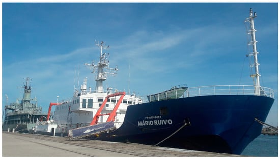
Figure 1.
Mário Ruivo research vessel.

Table 1.
Mário Ruivo main characteristics [13,14,15].
The layout of the AOS prototype is shown in Figure 2. A GNSS antenna plus an automatic weather station (AWS), which includes an anemometer, were placed on the highest deck right above the bridge. The Ferrybox equipped with a water pumping system and its own GNSS system was positioned just outside of the survey room. The onboard desktop computer (ODC) and monitor display, GNSS receiver, IMU and the indoor console of the AWS were installed in the survey room. All data were recorded in the ODC, serving as the central hub to which all sensors were connected, each with its dedicated software application and user interface. This system is based on the one installed by [3] and is totally autonomous (no human action) once initiated.
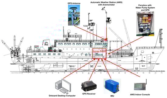
Figure 2.
AOS prototype layout onboard RV Mário Ruivo.
3.2. AOS Sensors and Ocean Waves Estimator Description
In this section, all the sensors and an ocean waves estimator [16] of the AOS prototype are described.
- Meteorological Unit: The AWS installed onboard the RV and shown in Figure 3a consists of three main systems: the integrated sensor suite (ISS) which houses and manages the external sensor array, the anemometer, and the indoor console data receiver and display. The wireless ISS is powered by a battery and a solar panel and acquires weather data from its array of sensors and anemometer, sending them via radio (Federal Communications Commission (FCC)-certified communication, license-free, spread-spectrum frequency hopping) to the wireless indoor console which is connected to the ODC using a data logger.
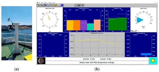 Figure 3. (a) AWS; (b) WeatherLink® user interface (weather bulletin).The ISS is equipped with a rain collector to measure the rainfall, the air temperature, and humidity sensors are mounted in a passive radiation shield to minimize the influence of solar radiation on sensor readings, and a barometric sensor. The anemometer measures the wind speed and direction [17,18].The AWS WeatherLink® software version 6.0.5 installed on the ODC allows for the configuration of the AWS sensors and records the collected weather data through the functionalities displayed in the user interface [19]. It uses the archive memory and a database to store weather data. The archive memory stores data records at each archive interval. When downloaded, all the weather data are transferred from the software’s archive memory to the database stored in the ODC disk. The software estimates the data for each weather function to arrive at an entry for the archive memory or database. The archive interval was set to 10 min and downloaded automatically every 5 min. The sampling rates and calculations are given in Table 2 for 10 min intervals. Additionally, specific technical data of the AWS are shown in Table 3.
Table 2. Sampling rates and calculations of weather functions for 10 min archive interval [19].Table 2. Sampling rates and calculations of weather functions for 10 min archive interval [19].
Figure 3. (a) AWS; (b) WeatherLink® user interface (weather bulletin).The ISS is equipped with a rain collector to measure the rainfall, the air temperature, and humidity sensors are mounted in a passive radiation shield to minimize the influence of solar radiation on sensor readings, and a barometric sensor. The anemometer measures the wind speed and direction [17,18].The AWS WeatherLink® software version 6.0.5 installed on the ODC allows for the configuration of the AWS sensors and records the collected weather data through the functionalities displayed in the user interface [19]. It uses the archive memory and a database to store weather data. The archive memory stores data records at each archive interval. When downloaded, all the weather data are transferred from the software’s archive memory to the database stored in the ODC disk. The software estimates the data for each weather function to arrive at an entry for the archive memory or database. The archive interval was set to 10 min and downloaded automatically every 5 min. The sampling rates and calculations are given in Table 2 for 10 min intervals. Additionally, specific technical data of the AWS are shown in Table 3.
Table 2. Sampling rates and calculations of weather functions for 10 min archive interval [19].Table 2. Sampling rates and calculations of weather functions for 10 min archive interval [19].Weather Function Sample Rate (Every) Temperature (average) 5 s Barometric pressure (1 reading) 10 min Wind speed (average) 5 s Wind direction (dominant) 5 s Relative humidity (average) Not specified
Table 3. Specific technical data of the AWS [17].Table 3. Specific technical data of the AWS [17].Weather Variables Resolution Accuracy Range Temperature 1 °C ±0.3 °C [−40, +65] °C Barometric Pressure 0.1 mmHg ±0.8 mmHg [410, 820] mmHg Wind Speed 1 knot 2 knots or 5% [0, 173] knots Wind Direction 22.5° ±3° 1–360° Humidity 1% ±2% 1–100% RH The software’s user interface displays the current and dominant wind directions on a compass rose and several measures of the wind speed, such as current and averaged values, as can be seen in Figure 3b. However, the AWS does not have inputs from a gyrocompass nor GNSS, and thus the wind speed and direction readings are relative to the vessel. Hence, the true wind speed and direction are estimated taking also into consideration the ship’s speed over ground (SOG) and course over ground (COG), obtained from GNSS data. To successfully ensure the correct estimation of the wind speed and direction values, the arm of the anemometer points to the bow of the vessel to set a reference, meaning that when the wind vane is pointing to the same direction of the arm, it is known that the reading is 0° or 360°. It is important to distinguish between true heading and COG, as the terms course and heading are used interchangeably, for example, in much of the literature on guidance, navigation, and control of marine craft, which leads to confusion [20].By definition, a ship’s heading at any given moment in time is the angle, expressed in degrees clockwise from north (0 degrees) of the ship’s fore-and-aft line relative to the true meridian or the magnetic meridian. In other words, it is the direction in which a vessel (its bow) is pointing at, being expressed as the angular distance relative to north, generally 0 degrees at north, clockwise through 359 degrees, of either true, magnetic, or compass direction. Therefore, true heading is when this angle is referred to the true meridian or geographical north. Generally, the heading estimation can be given by an IMU. In turn, the course is the intended direction of travel, which ideally (but seldom) is equal to the heading. As the heading, it is also expressed as the angular distance from north (0 degrees), clockwise. Additionally, the actual direction of the vessel’s motion or progress between two points, with respect to the surface of the earth, is named course over ground (COG), which can be provided by a GNSS receiver [21,22,23]. - Motion sensor unit: It is both a fibre-optic survey-grade IMO (International Maritime Organization)-certified gyrocompass and a motion reference unit for marine applications. It delivers true heading, roll, pitch, heave, surge, sway, rates of turn, and accelerations. Its core is a compact strapdown IMU containing three accelerometers, three fibre-optic gyrometers, and a real-time computer. The gyrometer has no moving parts, requiring neither maintenance nor recalibration. It provides a broad dynamic range and tolerates extremely demanding mechanical environments without compromise to its performances. Strapdown equation processing ensures that the system finds North in less than 5 min under any sea conditions. The IMU outputs directly binary data to the National Marine Electronics Association (NMEA) 0183 standard, which can be reconfigurable [24]. A short technical description is given in Table 4.
Table 4. Short technical description of the OCTANS IMU [24,25].Table 4. Short technical description of the OCTANS IMU [24,25].
Heading Values Dynamic accuracy ±0.2° Secant latitude Settle point error ±0.1° Secant latitude Repeatability ±0.025° Secant latitude Resolution 0.01° Settling time (static conditions) <1 min (full accuracy) Settling time at sea 1 <3 min (full accuracy) Speed compensation No limitation Latitude range No limitation Heave/Surge/Sway Values Accuracy 5 cm or 5% (highest of) Resolution 1 cm Heave motion periods 0.03 to 1000 s (tuneable) Roll/Pitch/Yaw Values Dynamic accuracy 0.01° (ind. from attitude) Range No limitation (±180°) Follow-up speed Up to 500°/s 1 Whatever sea-state (Secant lat. = 1/cos lat.).The unit is connected to the ODC via a USB to RS232 converter. The IMU was installed on the floor of the survey room, as seen in Figure 4a, as near as possible to the centre of gravity of the ship, and its relative position to the centre was recorded for the wave estimator calculations and correction of ship motions.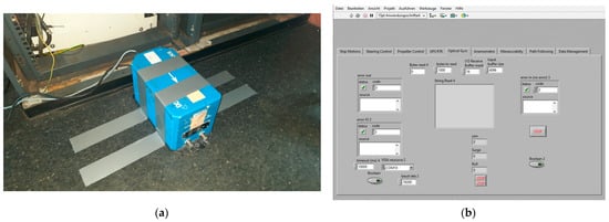 Figure 4. (a) IMU motion sensor in the survey room; (b) LabVIEW™ user interface for the IMU.The LabVIEW™ software 2018 version from National Instruments© installed on the ODC was programmed for acquiring and saving data automatically from the IMU and to provide a user interface, as shown in Figure 4b.
 - GNSS unit: This set has a next-generation receiver with high-performance global navigation satellite system (GNSS) positioning, and in the field, it is software-upgradable to provide the custom performance needed for application demands [26]. It provides scalable high precision positioning with ethernet, serial, USB, and controller area network (CAN) bus interfaces together with an application program interface (API) option to support custom applications. It can track all current and upcoming GNSS constellations and satellite signals, such as GPS, GLONASS, Galileo, and BeiDou [27]. A short technical description is given in Table 5. The receiver was installed in the survey room, as seen in Figure 5a, and the antenna was installed on the deck above the bridge. The software user interface installed on the ODC is shown in Figure 5b.
Table 5. Short technical description of the GNSS receiver [26].
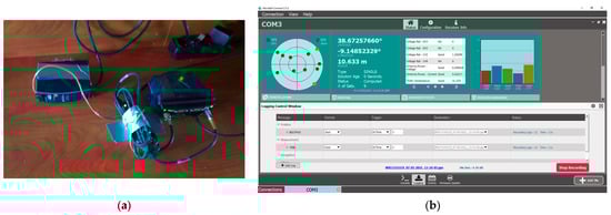 Figure 5. (a) GNSS receiver and power supply; (b) GNSS software (NovAtel Connect 2.3.2) user interface.
 - Ferrybox system: The surface oceanographic measurements were performed by a multi-sensor Ferrybox with a water pumping system and a GNSS system for geolocation. The measurements were obtained continuously during the full-scale trial route, and the core parameters were sea water temperature, pH, dissolved oxygen, total dissolved solids (TDS), conductivity, salinity, turbidity, chlorophyll-a, and phycocyanin. Having an in situ acquisition system provided real-time water surface oceanic data transmitted in real-time to the cloud platform through a 3G connection and antenna. Additionally, it integrated a GNSS receiver and antenna for accessing positional information. There was a screen on top of the box to control its operation. Being compact, the Ferrybox was small-sized (30 cm × 30 cm × 25 cm) and light-weighted (<6 kg), enabling its easy installation in a ship (e.g., VOO), which is an advantage over heavier Ferrybox-type devices. It was powered by the vessels’ electric grid and used an external water pump for sea water input and output having the inflow controlled through a flowmeter. Every time the Ferrybox was turned on, a clean freshwater inlet was activated to clean the sensors, preventing them from getting dirty [3]. The Ferrybox was installed in a box/enclosure/cabinet set right outside the survey room along with the connection to the power supply, water pump, installation pipes, and flowmeters for sea and freshwater inputs and output discharges (see Figure 2).
- Ocean Waves Estimator: This estimator algorithm was part of the AOS, and it ran on the ODC through a MATLAB® script and data from the IMU. The algorithm estimated the ship wave spectrum every 20 min using three ship motions data recorded with a 20 Hz frequency by the IMU, namely, heave, roll, and pitch. The estimator was based on the work by [28] and employed the pre-estimated vessel’s response amplitude operators (RAOs), which depends on the vessel hull’s geometry, ship SOG as well as on the measured ship motions to estimate the wave spectrum using genetic algorithms.Several assumptions are considered to simplify the estimation process, i.e., the ship responses are linear with the incident waves, the waves formulation considers deep water, the fixed position is taken coincident to the ship axis, and the ship motions can be estimated following the equation [29]where Sij are the ship responses, Φ the ship’s RAO, E the wave spectrum, ωe the wave encounter frequency, and β the wave direction. As a general statement, the wave spectrum is convoluted with certain response functions.Equation (2) can represent Equation (1) in a matrix form, where b is the cross-spectrum vector composed of real and imaginary parts of the cross-spectrum responses, A is the coefficient or system matrix of the products of the complex transfer functions, and w the Gaussian white noise sequence vector, with zero mean and variance.Essentially, the relationship between the measured response spectra and the directional wave spectrum is provided by Equation (2), as well as the information on the equivalence of energy. Without introducing white noise, no assumption is made on the error between the measured and the calculated response spectra, meaning that the directional wave spectrum can be sought in the least square sense by solving Equation (3).This optimization problem is solved by code based on genetic algorithms (GAs). The floating-point representation was chosen for all variables. The parameters that were problem-specific are shown in Table 6, as presented by [30].
Table 6. Considered genetic algorithm parameters.
- Onboard Desktop Computer (ODC): where all measured data are automatically collected and recorded in separate files for each sensor. It also provides the user interfaces and live readings of each sensor. The AOS is totally autonomous (no human intervention) after beginning to run. The ODC operates with a Microsoft Windows® 10 license, has an Intel® Core™ i3-2100 CPU at 3.1 GHz, 2 cores, 4 logical processors, a 64-bit operating system, 8 GB RAM, and a 250 GB solid-state drive (SSD).
3.3. AOS Tests Onboard the RV Mário Ruivo Description
Using the RV Mário Ruivo as a VOO, the AOS prototype installed onboard was tested during an oceanographic research campaign that took place between 23 and 26 of May 2021 (EMSO—European Multidisciplinary Seafloor and Water Column Observatory), along the southwest Portuguese coast. The aim was to collect meteorological, oceanographic, and ship motions data during the research campaign based on the AOS installed onboard.
The start and end of the ship route were in the Naval base of Alfeite in Lisbon. The ship sailed south along the Portugal coast down to Algarve’s coast, collecting data in that area and returning afterwards to Lisbon along the coast.
Figure 6a shows a plot of a section of the vessel’s route when returning to Lisbon during the campaign. Data were acquired over a duration of around 28.5 h between 09:14:03 on 25 May 2021 and 13:49:00 on 26 May 2021 from a location with latitude ≈ 36.95° N and longitude ≈ 9.70° W to a location with latitude ≈ 38.40° N and longitude ≈ 9.27° W. GNSS data were validated using a second GNSS receiver installed onboard. The plot was generated after the development of a Python script using the folium package and the GNSS data.
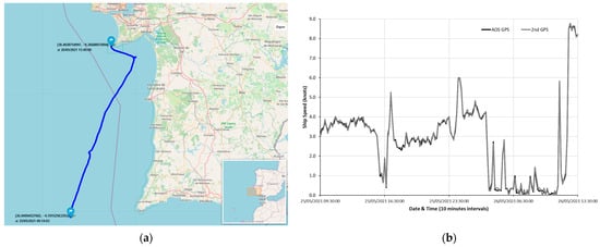
Figure 6.
(a) Section of the RV route along the southwest coast of Portugal; (b) RV’s speed estimated from the AOS GNSS and second GNSS data.
The RV’s SOG validation was made by comparing speed estimations from both GNSS data, which are represented in the plot of Figure 6b. The difference between the speed values estimated from the AOS GNSS and the second GNSS has a mean value of only 0.09 knots and a standard deviation of 0.06 knots.
This validation is important, not only for determining the vessel’s route but also for calculating the true wind speed and for the wave spectrum estimator. The speed estimation involved GNSS data collected from 09:20:00, on 25 May 2021, to 13:30:00, on 26 May 2021, with intervals of 10 min resolution. Data were processed using a developed MATLAB® script, which transforms the geodetic data coordinates (latitude, longitude, altitude) into the Earth-centered, Earth-fixed (ECEF) coordinate system, also known as geocentric coordinate system. These transformations are based on the equations outlined in Section 10.2 of reference [31].
4. Results of the Full-Scale Trial
In this section, the results related to the meteorological and wave and parameters are presented and analysed. The results derived from the Ferrybox system will be addressed in a forthcoming paper.
The meteorologic experimental results were obtained from the readings of the AWS. The true wind speed and direction estimates were derived from the anemometer data complemented by measurements from the motion sensor and GNSS units. These results were validated through a comparison with data obtained from a second set of sensors installed onboard the RV.
4.1. Meteorological Parameters
The meteorological parameters measured by the AWS include air temperature, relative humidity, barometric pressure, and wind speed and direction. The measurements cover the period from 09:20:00 on 25 May 2021 to 13:30:00 on 26 May 2021, corresponding to the selected route section of the research campaign, as depicted in Figure 6a.
The AWS is configured to measure all the parameters with 10 min intervals, with the software outputting their averaged values, except for the barometric pressure and wind direction. The pressure data are sampled once at the end of each interval, while wind direction measurements, although taken as frequently as wind speed within the sampling interval, are categorized by the software into the respective “bins”. These bins correspond to the sixteen compass points, each spanning a range of 22.50°. This categorization occurs if the wind speed exceeds zero. At the end of the 10 min interval, the software identifies the predominant wind direction bin by determining which bin contains the highest number of values [19].
Figure 7a–d shows the plots of 10 min intervals data measured by the AOS automatic weather station and the second weather station for the following meteorologic parameters, respectively: average air temperature; average relative humidity; barometric pressure; and true wind speed.
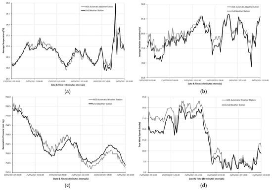
Figure 7.
Data of the following meteorologic parameters from both weather stations: (a) average air temperature; (b) average relative humidity; (c) barometric pressure; (d) true wind speed.
The differences between both weather stations’ values for these parameters are given in Table 7. The means and standard deviations values are acceptably low, which validates the readings. It should be mentioned that the true wind speed parameter has the highest mean difference and standard deviation, considering the range of its measured values. Upon observing Figure 7d, the curves have a similar behaviour, and although differences between their values are larger in the first half of the plot, they converge approximately to the same values afterwards. This might have to do with the fact that both weather stations were placed around 5 m apart of each other and fixed into different structures of the deck above the bridge, which may differently affect locally the wind readings. Indeed, proper locations for wind sensors are particularly difficult to find as most sites for an anemometer to be placed will be affected by wind flow distortion over the superstructure [11].
Table 7.
Differences between both weather stations values for the four parameters.
Figure 7 and Table 7 show the performance of two sets of sensors. The data were collected to allow the assessment of the uncertainties than can be expected when using such types of equipment.
It is worth noting that the AWS’s anemometer automatically gives the apparent wind only, i.e., the wind relative to the anemometer’s arm (vessel framework). Thus, to obtain the true wind speed, the following was performed:
- The anemometer’s arm was pointed to the bow of the ship upon its installation. This way, when the measured value of the apparent wind direction was 0° or 360°, the direction of the wind was known to be aligned with the ship’s bow.
- The ship’s speed was estimated from the AOS GNSS data.
- The true wind speed was obtained by subtracting the vessel’s SOG vector to the apparent wind speed vector given by the AWS anemometer, taking into account that the apparent wind direction was known, i.e., the angle of this vector relative to the ship’s bow.
4.2. Oceanographic Waves Parameters
The oceanographic wave parameters and wave spectrum were estimated by the ocean wave estimator using genetic algorithms for a set of three selected locations along the RV’s route, as indicated in Figure 8. The estimations make use of the pre-estimated vessel’s RAO, which depends on the ship hull’s geometry, the ship’s SOG at the locations, and ship motions (heave, roll, and pitch) for 20 min of the IMU data in and near the locations, considering the correction due to the distance from where the IMU was placed in the bridge to the RV’s centre of gravity. The locations were chosen for the highest ship motions’ amplitudes. The estimation procedure is based on the method presented in [16] and detailed in point 4 of Section 3.2 of the current paper.
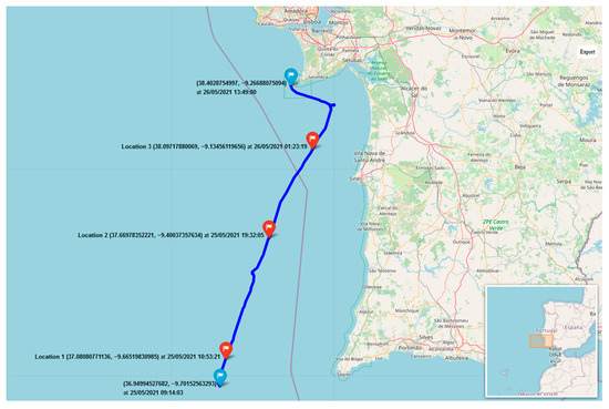
Figure 8.
Three locations along the vessel’s route.
The estimator outputted the wave spectra, in polar form, and the following wave parameters: significant wave height (Hs in meters); peak wave period (Tp in seconds); peak intensification factor (γ); mean wave direction relative to the vessel’s stern (β in degrees); and wave spreading factor.
The estimations are validated against the forecasted data from the Copernicus’ ERA5 database containing hourly data on single levels from 1959 to the present [32]. This ERA5 database is the fifth generation of the European Centre for Medium-Range Weather Forecasts (ECMWF) reanalysis for global climate and weather for the past decades, providing hourly estimates for a considerable set of atmospheric, ocean-wave, and land-surface parameters. The reanalysis product combines model data with worldwide observations into a globally complete and consistent dataset using the laws of physics, a principle named data assimilation, based on the method employed by numerical weather prediction centres. The dataset is a regridded subset of the complete ERA5 dataset on native resolution [33]. The selected forecasted parameters for our case are the significant height of combined wind waves and swell (Hs), peak wave period (Tp), and true north mean wave direction (β). A short description of these ERA5 parameters is given [33]:
- Significant height of combined wind waves and swell (Hs): This represents the mean height in meters of the highest third of surface ocean/sea waves produced by local winds and the related swell (this parameter takes both into account), meaning the vertical distance between the wave crest and wave trough. It is a parameter which is four times the square root of the integral over all directions and frequencies of the 2D wave spectrum.
- Peak wave period (Tp): This represents the period in seconds of the most energetic oceans waves produced by local winds and the related swell (this parameter takes both into account), being calculated from the reciprocal of the frequency associated with the largest value (peak) of the frequency wave spectrum.
- (True) mean wave direction (β): This represents the mean direction in degrees true of the ocean/sea surface waves generated by local winds and swell (this parameter takes both into account), consisting in the mean over all frequencies and directions of the 2D wave spectrum. The degrees true mean the direction relatively to the North Pole geographic location. It is the direction that waves are coming from. Thus, 0 and 90 degrees mean “coming from the North” and “coming from the East”, respectively.
These three parameters’ NetCDF data files were downloaded from the aforementioned database containing hourly data and using the reanalysis product. The chosen dates and times (UTC—universal time coordinated) for the data were based on the closest ones to each location in Figure 8. It is important to refer that the time zone at the locations in May is UTC + 1. So, for example, location 1 AOS GNSS and IMU data are from 10:53:21 AM UTC + 1, which led to selecting Copernicus ERA5 data from 10:00 AM UTC, i.e., meaning 11:00 AM in UTC + 1 time zone of location 1.
The NetCDF files of these parameters have a latitude-longitude grid of 0.5 × 0.5 degrees for the reanalysis. Afterwards, climate data operators (CDOs) commands were used in a Windows® Cygwin64© terminal for regridding to 0.01 × 0.01 degrees.
Figure 9 shows the ship motions, heave, roll, and pitch for a period of 20 min IMU readings when the RV was passing through location 1. These ship motions were based on the IMU’s data and corrected by considering the distance from the IMU to the vessel’s centre of gravity. This approach is also used for ship motions at locations 2 and 3.
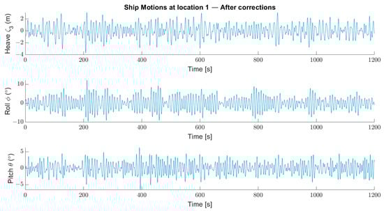
Figure 9.
Ship motions, heave, roll, and pitch for 20 min IMU readings in and near location 1 corrected by considering the distance of the IMU relatively to the vessel’s centre of gravity.
The recorded ship motions are high. The highest roll values are over 10 degrees at locations 1 and 2, and the heave motions reach values higher than 3 m at location 1, all due to the bad weather experienced at that time. The length of the time series is 20 min, which can be considered a constant sea state.
Figure 10a presents the estimated wave spectrum in polar form for location 1 considering the 20 min corrected ship motions, whereas Figure 10b shows the forecasted significant height of the combined wind waves and swell at the same location obtained from data from the Copernicus database and using the Panoply netCDF, HDF and GRIB Data Viewer running on Windows® platform [34]. This approach is also used for data of locations 2 and 3.
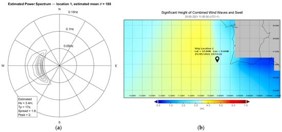
Figure 10.
For location 1: (a) estimated wave spectrum over 20 min of corrected ship motions; (b) forecasted significant height of combined wind waves and swell based on data from Copernicus.
At location 1 and looking to Figure 10a, the estimated wave spectrum has a significant wave height Hs = 3.4 m, wave period Tp = 16.8 s, and mean wave direction θ = 188° (with respect to the ship stern). The estimated wave spectra have good agreement for the significant wave height as they are approximately the same as the forecasted ones (see Figure 10b), as can be seen in Table 8. But, in the estimation of the wave period and mean wave direction, some errors arise since the minimization function depends on the energy content below the power curve. The directional spectra not only consider the three parameters discussed before but also depend on the spreading function and peak enhancement factor γ. The estimated wave direction is 188° which indicates the ship encountered head waves, thus meaning predominant heave and pitch ship motions as can be observed in the corrected IMU measurements in Figure 9.
Table 8.
Set of forecasted and estimated wave parameters for the three vessel’s locations.
At location 2, the estimated mean wave direction is close to 180°, which indicates the ship encountered head waves, thus meaning predominant heave and pitch ship motions occurred, as can be observed in the corrected IMU measurements in Figure 11. Looking to Figure 12a, the estimated wave spectrum has a significant wave height Hs = 2.9 m, wave period Tp = 17 s, and mean wave direction θ = 171° (with respect to the ship stern). The estimated wave spectra have good agreement for the significant wave height when compared to the forecasted ones (see Figure 12b), but in the estimation of the wave period, the errors are high (see Table 8), since the minimization function depends on the energy content below the power curve.
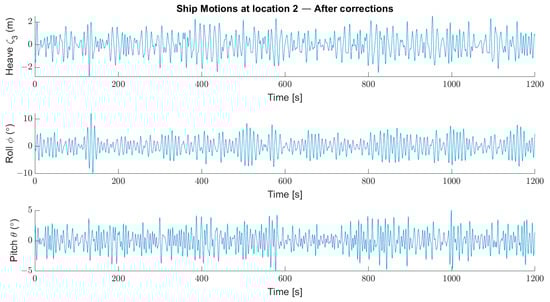
Figure 11.
Ship motions, heave, roll, and pitch for 20 min IMU readings in and near location 2 corrected by considering the distance of the IMU relatively to the vessel’s centre of gravity.
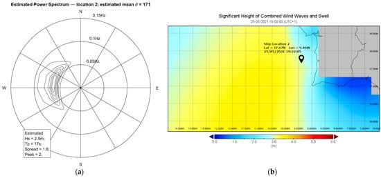
Figure 12.
For location 2: (a) estimated wave spectrum over 20 min of corrected ship motions; (b) forecasted significant height of combined wind waves and swell based on data from Copernicus.
At location 3, the estimated mean wave direction is 285°, which indicates the ship encountered beam waves, thus meaning the roll motions are higher than the heave and pitch motions, as can be observed in the corrected IMU measurements in Figure 13. Looking at Figure 14a, the estimated wave spectrum has a significant wave height Hs = 2.3 m, Tp = 15 s and mean wave direction θ = 285° (with respect to the ship stern). The estimated wave spectra have good agreement for the significant wave height and wave period (see Table 8).
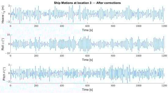
Figure 13.
Ship motions, heave, roll, and pitch for 20 min IMU readings in and near location 3 corrected by considering the distance of the IMU relatively to the vessel’s centre of gravity.
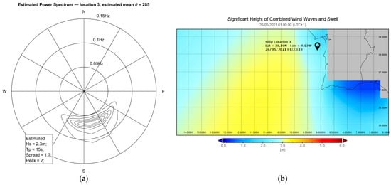
Figure 14.
For location 3: (a) estimated wave spectrum over 20 min of corrected ship motions; (b) forecasted significant height of combined wind waves and swell based on data from Copernicus.
Table 8 presents, for all three locations, the estimated results from the wave spectrum estimator and forecasted values from the Copernicus database for several wave parameters, namely, significant wave height, peak wave period, peak intensification factor, mean wave direction, and wave spreading factor. The wave estimation algorithm considers combined wind waves and swell.
The method that estimates the wave spectrum, which basically estimates the spectrum energy, depends on the assumption of a parametric representation of the wave spectrum. In this study, the model used is the well-known JONSWAP spectrum. This model has five parameters, namely, the significant wave height, wave period, wave direction, spread function, and peak factor. The errors related to the estimation of one of those parameters are subjected to the estimation of the others. Thus, in our estimations, the errors obtained for the significant wave height are low, which affects the estimations in the wave period.
The wave spectrum estimator has, as a reference frame, the ship axis coordinates, where the positive x-direction is equivalent to head waves (180°). The Copernicus database reference frame axis is based on true north (north is equivalent to 0°).
The errors given in Table 8 for significant wave height and wave period are calculated by
The error in wave direction is the difference between the forecasted and estimated data (θ in Figure 10a, Figure 12a and Figure 14a). From Table 8, it is possible to see errors around 30° for locations 1 and 2. These errors are acceptable considering that the estimation algorithm and the vessel’s RAO have a 20 degrees grid. The following is an example of the error calculation for the wave direction:
- Location 1: 188° relatively to the vessel’s stern, as seen in Figure 10a (equivalent to 172° due to ship symmetry), and 14° true heading (from IMU). So, the wave direction is 180° − 172° = 8° starboard relatively to the bow, and we must add it to the 14° true heading, giving 14° − 8° = 6° true wave direction. Therefore, the error is (|Forecasted − Estimated|) = |336° − (360° + 6°)| = 30°.
5. Discussion
The data and results obtained from the full-scale trial have shown that the presented AOS prototype can be a feasible approach to collect and integrate meteorological and oceanographic data obtained onboard a VOO.
The meteorological parameters measured by the AWS over 10 min archive intervals were validated against the readings of a second weather station. The differences between the mean values of both stations were 0.11 °C, 1.63%, 0.22 mmHg, and 2.96 knots for the average temperature, average relative humidity, barometric pressure, and true wind speed, respectively. The standard deviations were of the same order of magnitude. These values are reasonably low, thus validating the readings.
Oceanographic wave parameters and wave spectra were estimated by an ocean wave estimator, using genetic algorithms for optimization and a short computational time, for three selected locations along the RV’s route. The estimator outputted the wave spectra, in polar form, and wave parameters such as the significant wave height, peak wave period, peak intensification factor, mean wave direction, and wave spreading factor. Estimations relied, at each location, on the ship’s SOG and on 20 min of IMU ship motions data (heave, roll, and pitch), corrected due to the distance of the IMU to the RV’s centre of gravity. These estimations were validated with forecasted wave data from the Copernicus’ ERA5 database.
The results of the wave estimator for the significant wave height have good agreement with the forecasted ones from the Copernicus database as the errors are below 3%. The errors for the wave period are around 16–28%, which is reasonable for one of the locations, but in the other two, the errors are higher since the minimization function depends on the energy content below the power curve. Moreover, the errors associated with the estimation of one of these parameters are subjected to the estimation of the others. Consequently, the errors obtained in the estimations for the significant wave height are low, which affects the estimations in the wave period. Concerning the mean waves directions, the errors are between 30° and 45°, but for two of the locations, the errors are acceptable, given that the estimation algorithm and the vessel’s RAO have a 20 degrees grid. Additionally, the estimated mean waves directions are in accordance with the effects of the waves in the ship motions (heave, pitch, roll) observed in the corrected measurements of the IMU. An improvement would involve developing an algorithm to conduct online validations with the NOAA database.
6. Conclusions
The current paper describes an AOS prototype consisting of an AWS, IMU, and a GNSS unit installed onboard a Portuguese RV and shows the respective underway measurements obtained during a full-scale trial off the coast of Portugal along with wave parameters estimated with an ocean wave estimator.
The presented AOS prototype demonstrated its potential as a feasible approach for collecting quality environmental data, integrating meteorological and oceanographic data collected onboard VOO. The system has been designed to be installed in fishing vessels that will operate as VOO and as a distributed network of ocean data collection.
While data such as wind speed and wave height can be obtained from weather satellites, the information collected by VOO plays a crucial role in not only confirming the accuracy of remotely acquired data but also in validating and enhancing the results of computer numerical models [35], such as the ones used in larger and mesoscale scientific climate studies, and also in smaller coastal scale projects, such as the ones related to coastal ocean engineering works (e.g., ports construction, renewable offshore winds, and waves energy).
The AWS and the anemometer are self-contained pieces of equipment powered by a lithium battery and a solar panel, with large autonomy lasting around two years with the same battery [18]. Additionally, the communication between the AWS and its indoor console connected to the ODC is wireless, simplifying the installation and maintenance, given that there is no need for cabling.
The wave estimator using an IMU can be a cost-effective alternative solution to wave radars, as the IMUs can be cheaper and be installed indoors in the ship’s bridge away from the harsh maritime environment, reducing the need for difficult installations of a radar on top of the mast or on the ship’s bow plus long cablings, reducing maintenance time and costs and acquisition costs, given that wave radars are quite expensive. Improvements of the wave estimator algorithm for enhanced accuracy can be possible with more testing of the AOS after its installation in fishing vessels working as VOO for ocean data collection.
Author Contributions
The autonomous observing system was designed by A.M.P.-S. and C.G.S.; the implementation of the observing system and field work was performed by A.M.P.-S., F.P.S., T.L.R. and R.V.; tests onboard RV Mário Ruivo were carried by T.L.R.; data processing was carried out by F.P.S. and M.A.H.; original draft writing, preparation, and editing was carried by all authors, namely, Introduction: F.P.S. and T.L.R.; Materials and Methods: F.P.S., T.L.R., M.A.H., R.V. and A.M.P.-S.; Results: F.P.S. and M.A.H.; Discussion: F.P.S., T.L.R., M.A.H. and C.G.S. All authors have read and agreed to the published version of the manuscript.
Funding
This research was funded by the EU FEDER/FEMP and Portuguese Foundation for Science and Technology (FCT) under the Portugal2020 (Lisboa2020, Algarve2020 and MAR2020) Programme through projects OBSERVA.FISH (PTDC/CTA-AMB/31141/2017) and OBSERVA.PT (MAR-01.04.02-FEAMP-0002). This work contributes to the Strategic Research Plan of the Centre for Marine Technology and Ocean Engineering (CENTEC) and of the Centre of Marine Sciences of the University of Algarve (CCMAR) which are financed by the Portuguese Foundation for Science and Technology (FCT) under contract UIDB/UIDP/00134/2020, and UIDB/04326/2020 (DOI:10.54499/UIDB/04326/2020), UIDP/04326/2020 (DOI:10.54499/UIDP/04326/2020) and LA/P/0101/2020 (DOI:10.54499/LA/P/0101/2020).
Institutional Review Board Statement
Not applicable.
Informed Consent Statement
Not applicable.
Data Availability Statement
Data are contained in the article.
Acknowledgments
The authors would like to express their appreciation to Shan Wang of the Centre for Marine Technology and Ocean Engineering (CENTEC) for the support in the estimations of the RAOs and to the RV Mário Ruivo crew for all the support in the installation of the sensors in the vessel as well as for supplying the structural drawings of the ship.
Conflicts of Interest
The authors declare no conflicts of interest.
Acronym/Abbreviation
| AOS | Autonomous Observing System |
| API | Application Program Interface |
| AWS | Automatic Weather Station |
| CAN | Controller Area Network |
| CDO | Climate Data Operator |
| CENTEC | Centre for Marine Technology and Ocean Engineering |
| COG | Course Over Ground |
| ECEF | Earth-Centred, Earth-Fixed |
| ECMWF | European Centre for Medium-Range Weather Forecasts |
| ECV | Essential Climate Variable |
| EMSO | European Multidisciplinary Seafloor and Water Column Observatory |
| EOV | Essential Ocean Variable |
| FCC | Federal Communications Commission, A United States (US) Federal Government Agency to Regulate All Forms of Telecommunications Inside of the US |
| GA | Genetic Algorithms |
| GCOS | Global Climate Observing System |
| GNSS | Global Navigation Satellite System |
| GOOS | Global Ocean Observing System |
| GPS | Global Positioning System |
| GSM | Global System for Mobile Communications |
| GTS | Global Telecommunication System of WMO |
| GTSPP | Global Temperature–-Salinity Profile Program |
| ICOADS | International Comprehensive Ocean–Atmosphere Data Set |
| IMO | International Maritime Organization |
| IMU | Inertial Measurement Unit |
| IOC | Intergovernmental Oceanographic Commission |
| IODE | International Oceanographic Data and Information Exchange |
| IoT | Internet of Things |
| IPMA | Portuguese Institute for Sea and Atmosphere |
| ISS | Integrated Sensor Suite |
| JCOMM | Joint Technical Commission for Oceanography and Marine Meteorology |
| JCOMMOPS | Jcomm Observing Programme Support |
| LoRa | Long Range |
| MDC | Marine Data Centre of Florida State University |
| NMEA | National Marine Electronics Association |
| NMHS | National Meteorological and Hydrographic Service |
| NOAA | National Oceanic and Atmospheric Administration |
| OCG | Observation Coordination Group |
| ODAS | Ocean Data Acquisition System |
| ODC | Onboard Desktop Computer |
| OWS | Ocean Weather Station |
| QC | Quality Control at MDC |
| RAO | Response Amplitude Operator |
| RV | Research Vessel |
| SAMOS | Shipboard Automated Meteorological and Oceanographic System |
| SOG | Speed Over Ground |
| SOOP | Ships of Opportunity Program |
| SOT | Ship Observations Team |
| SSD | Solid-State Drive |
| TDS | Total Dissolved Solids |
| UNESCO | United Nations Educational, Scientific, and Cultural Organization |
| UOT | Upper Ocean Thermal |
| UTC | Universal Time Coordinated |
| VOO | Vessels of Opportunity |
| VOS | Voluntary Observing Ship |
| VOSClim | Vos Climate Fleet |
| WMO | World Meteorological Organization |
| WWI | World War I |
| WWII | World War Ii |
References
- Davis, R.E.; Talley, L.D.; Roemmich, D.; Owens, W.B.; Rudnick, D.L.; Toole, J.; Weller, R.; McPhaden, M.J.; Barth, J.A. 100 Years of Progress in Ocean Observing Systems. Meteorol. Monogr. 2019, 59, 3.1–3.46. [Google Scholar] [CrossRef]
- Allen, S.; Wild-Allen, K. Ocean In Situ Sampling and Interfaces with other Environmental Monitoring Capabilities. In Challenges and Innovations in Ocean In Situ Sensors. Measuring Inner Ocean Processes and Health in the Digital Age; Delory, E., Pearlman, J., Eds.; Elsevier: Amsterdam, The Netherlands, 2019; pp. 1–26. [Google Scholar]
- Rosa, T.L.; Piecho-Santos, A.M.; Vettor, R.; Guedes Soares, C. Review and Prospects for Autonomous Observing Systems in Vessels of Opportunity. J. Mar. Sci. Eng. 2021, 9, 366. [Google Scholar] [CrossRef]
- Smith, S.; Alory, G.; Andersson, A.; Asher, W.; Baker, A.; Berry, D.; Schuster, U.; Steventon, E.; Vinogradova-shiffer, N. Ship-based contributions to global ocean, weather, and climate observing systems. Front. Mar. Sci. 2019, 6, 434. [Google Scholar] [CrossRef]
- Smith, R.S.; Briggs, K.; Bourassa, M.A.; Elya, J.; Paver, C.R. Shipboard automated meteorological and oceanographic system data archive: 2005–2017. Geosci. Data J. 2018, 5, 73–86. [Google Scholar] [CrossRef]
- Smith, R.S.; Lopez, N.; Bourassa, M.A. Samos air-sea fluxes: 2005–2014. Geosci. Data J. 2016, 3, 9–19. [Google Scholar] [CrossRef]
- Freeman, E.; Woodruff, S.D.; Worley, S.J.; Lubker, S.J.; Kent, E.C.; Angel, W.E.; Berry, D.I.; Brohan, P.; Eastman, R.; Gates, L.; et al. ICOADS Release 3.0: A major update to the historical marine climate record. Int. J. Climatol. (CLIMAR-IV Spec. Issue) 2017, 37, 2211–2237. [Google Scholar] [CrossRef]
- JCOMM. Voluntary Observing Ship Scheme. Ship Observations Team JCOMM. 2015. Available online: http://sot.jcommops.org/vos/documents/VOS-Poster-2015.pdf (accessed on 1 January 2023).
- VOS. Voluntary Observing Ship Scheme. 2022. Available online: http://sot.jcommops.org/vos/index.html (accessed on 1 January 2023).
- VOS. The JCOMM Voluntary Observing Ship Scheme, and Enduring Partnership. 2015. Available online: http://sot.jcommops.org/vos/documents/VOS-Brochure-2015.pdf (accessed on 1 January 2023).
- JCOOM VOS. International VOS Scheme. 2021. Available online: http://sot.jcommops.org/vos/vos.html (accessed on 1 January 2023).
- Goni, G.; Roemmich, D.; Molinari, R.; Meyers, G.; Sun, C.; Boyer, T.; Baringer, M.; Gouretski, V.; DiNezio, P.; Reseghetti, F.; et al. The Ship of Opportunity Program. Proceedings of OceanObs09’: Sustained Ocean Observations and Information for Society, Vol. 2, Venice, Italy, 21–25 September 2009; Hall, J., Harrison, D.E., Stammer, D., Eds.; ESA Publication WPP-306. European Space Agency (ESA): Roma, Italy, 2010. [Google Scholar] [CrossRef]
- IPMA. “Mario Ruivo”—Arranjo Geral Final. 2018. Available online: https://marioruivo.ipma.pt/wp-content/uploads/2021/10/Arranjo_Geral_Mario-Ruivo.pdf (accessed on 8 May 2021).
- IPMA. Mário Ruivo. 2022. Available online: https://marioruivo.ipma.pt/ (accessed on 2 August 2022).
- IPMA. R.V. Mário Ruivo Infographic. 2022. Available online: https://www.ipma.pt/export/sites/ipma/bin/docs/publicacoes/pescas.mar/navios/RV_MarioRuivo_Infographic.pdf (accessed on 2 August 2022).
- Hinostroza, M.A.; Santos, F.P.; Vettor, R.; Rodrigues, M. Preliminary results of a real-time weather and ship motion onboard monitoring system and data recording for a container ship. In Trends in Maritime Technology and Engineering; Guedes Soares, C., Santos, T.A., Eds.; Taylor & Francis Group: London, UK, 2022; Volume 1, pp. 583–592. [Google Scholar]
- Davis. Wireless Vantage Pro2 & Vantage Pro2 Plus Stations. DS6152_62_53_63 (Rev DD 4/14/20). 2020. Available online: https://cdn.shopify.com/s/files/1/0515/5992/3873/files/6152_62_53_63_ss.pdf?v=1623783718 (accessed on 30 April 2021).
- Davis. Integrated Sensor Suite—User Manual. Document Part Number: 7395.333 Rev J (7/27/20). 2020. Available online: https://cdn.shopify.com/s/files/1/0515/5992/3873/files/07395-333_IM-6322C-6334.pdf (accessed on 5 May 2021).
- Davis. Weatherlink for Windows—Software User’s Guide. Version 4.0, Product Number: 7862, Davis Instruments Part Number: 7395-121, Rev. C Manual. 1999. Available online: http://www.davis-tr.com/Downloads/WeatherLink_for_Windows_4.0_7862_Instruction_Manual.pdf (accessed on 5 May 2021).
- Fossen, T.I. Kinematics. In Handbook of Marine Craft Hydrodynamics and Motion Control, 1st ed.; John Wiley & Sons Ltd.: Chichester, West Sussex, UK, 2011; pp. 15–44. [Google Scholar]
- Bowditch, N. Compasses. In American Practical Navigator—An Epitome of Navigation, 54th ed.; Clifford, G.J., Ed.; National Geospatial—Intelligence Agency: Springfield, VA, USA, 2017; Volume I, pp. 133–152. [Google Scholar]
- Trimble Applanix. Course, Heading, and Bearing. News/Blog. 2024. Available online: https://www.applanix.com/news/blog-course-heading-bearing/ (accessed on 1 February 2024).
- Garmin. GPS Heading and Heading on a Garmin Marine Device. Support Center. 2024. Available online: https://support.garmin.com/sv-SE/?faq=kmZQtYAFUS32zpC08OIIcA. (accessed on 1 February 2024).
- IXSEA. User guide—OCTANS SURFACE, A ed.; ISXEA: Marly-le-Roi, France, 2004; pp. 35–38. [Google Scholar]
- IXSEA. OCTANS (Gyrocompass and Motion Sensor)—Navigation and Positioning. 2003. Available online: http://www.oceandata.co.kr/GroupWare/Home/product/brochure/ixsea/Octans.pdf (accessed on 19 August 2021).
- NovAtel. Enclosures FlexPak6™. D15802 May 2014. 2014. Available online: https://hexagondownloads.blob.core.windows.net/public/Novatel/assets/Documents/Papers/FlexPak6/FlexPak6.pdf (accessed on 1 May 2021).
- NovAtel. OEM6® Family—Installation and Operation User Manual. Publication Number OM-20000128, Revision Level 12, Revision Date October 2016. 2016. Available online: https://hexagondownloads.blob.core.windows.net/public/Novatel/assets/Documents/Manuals/om-20000128/om-20000128.pdf (accessed on 19 May 2021).
- Hinostroza, M.A.; Guedes Soares, C. Parametric estimation of the directional wave spectrum from ship motions. Int. J. Marit. Eng. 2016, 2, 121–130. [Google Scholar] [CrossRef]
- Bhattacharyya, R. Dynamics of Marine Vehicles; Wiley: New York, NY, USA, 1978. [Google Scholar]
- Pascoal, R.; Guedes Soares, C.; Sørensen, A.J. Ocean wave spectral estimation using vessel wave frequency motions. J. Offshore Mech. Arct. Eng. 2007, 129, 90–96. [Google Scholar] [CrossRef]
- Hofmann-Wellenhof, B.; Lichtenegger, H.; Collins, J. Global Positioning System—Theory and Practice, 5th ed.; Springer: Vienna, Austria, 2001; pp. 279–280. [Google Scholar] [CrossRef]
- Copernicus. Copernicus ERA5 Hourly Data on Single Levels from 1959 to Present—Download Data. 2022. Available online: https://cds.climate.copernicus.eu/cdsapp#!/dataset/reanalysis-era5-single-levels?tab=form (accessed on 12 October 2022).
- Copernicus. Copernicus ERA5 Hourly Data on Single Levels from 1959 to Present—Overview. 2022. Available online: https://cds.climate.copernicus.eu/cdsapp#!/dataset/reanalysis-era5-single-levels?tab=overview (accessed on 12 October 2022).
- Nasa. Panoply netCDF, HDF and GRIB Data Viewer. 2022. Available online: https://www.giss.nasa.gov/tools/panoply/ (accessed on 12 October 2022).
- Meteorological. All Aboard. In Meteorological Technology International—The International Review of Weather, Climate and Hydrology Technologies and Services; Norman, H., Symonds, D., Baker, E., Eds.; UKI Media & Events: Surrey, UK, 2020; pp. 42–44. Available online: https://www.ukimediaevents.com/publication/b853e52b/1 (accessed on 1 February 2024).
Disclaimer/Publisher’s Note: The statements, opinions and data contained in all publications are solely those of the individual author(s) and contributor(s) and not of MDPI and/or the editor(s). MDPI and/or the editor(s) disclaim responsibility for any injury to people or property resulting from any ideas, methods, instructions or products referred to in the content. |
© 2024 by the authors. Licensee MDPI, Basel, Switzerland. This article is an open access article distributed under the terms and conditions of the Creative Commons Attribution (CC BY) license (https://creativecommons.org/licenses/by/4.0/).