
Continuous Zonal Gradients Characterize Epipelagic Plankton Assemblages and Hydrography in the Subtropical North Atlantic


Abstract
1. Introduction
2. Materials and Methods
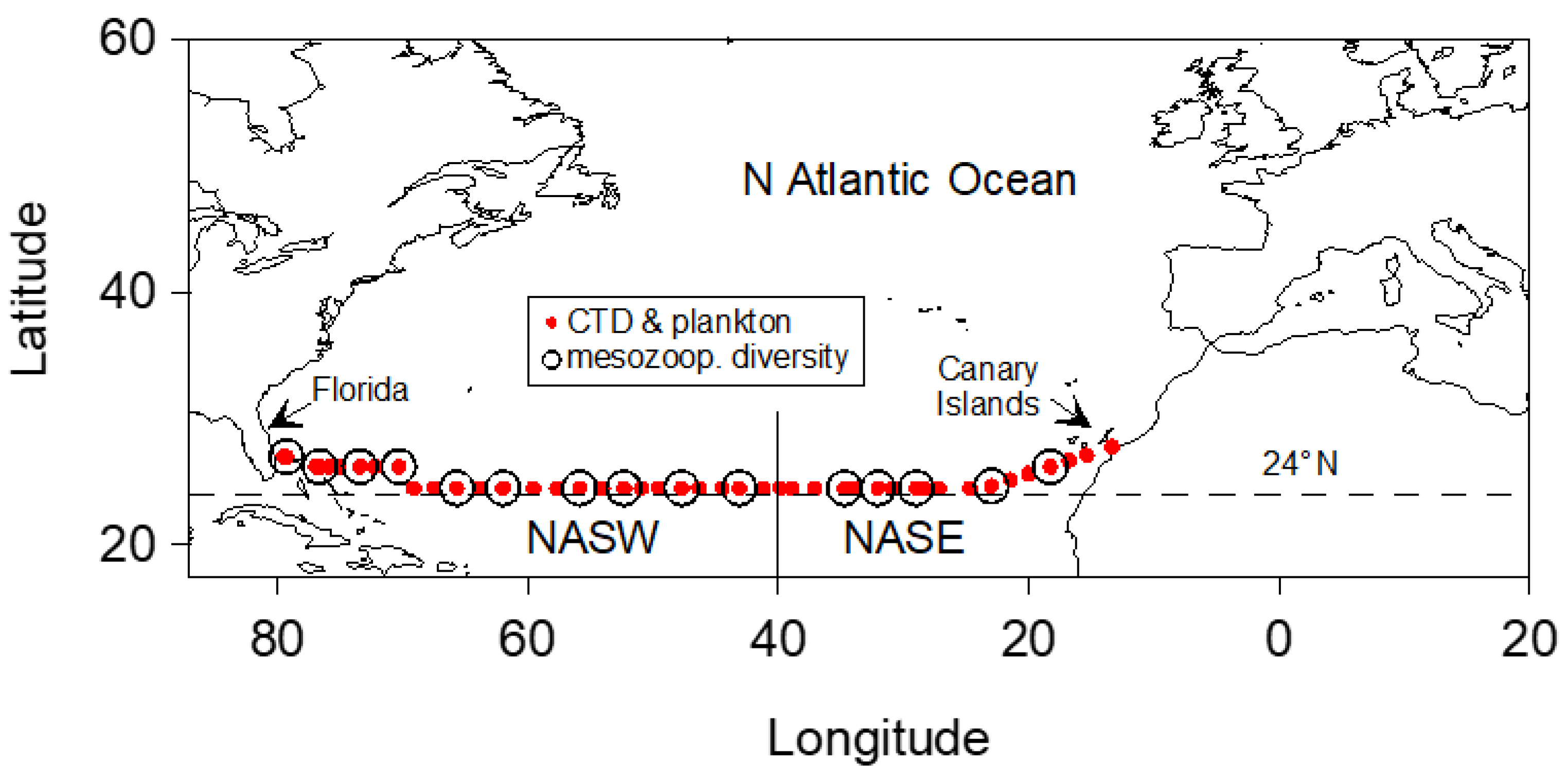
2.1. Sampling and Hydrographic Observations
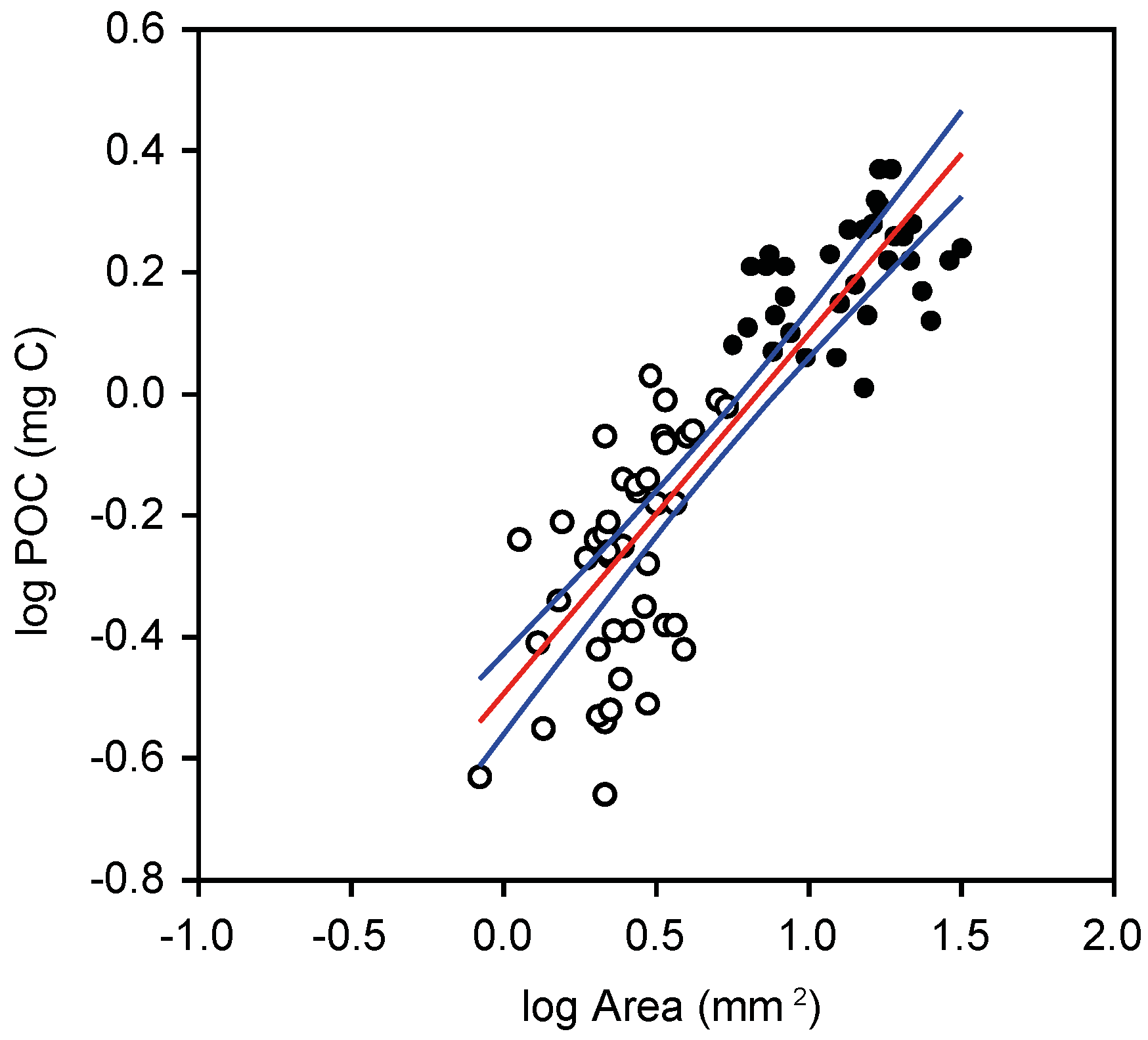
2.2. Plankton Abundance, Individual Size, and Composition
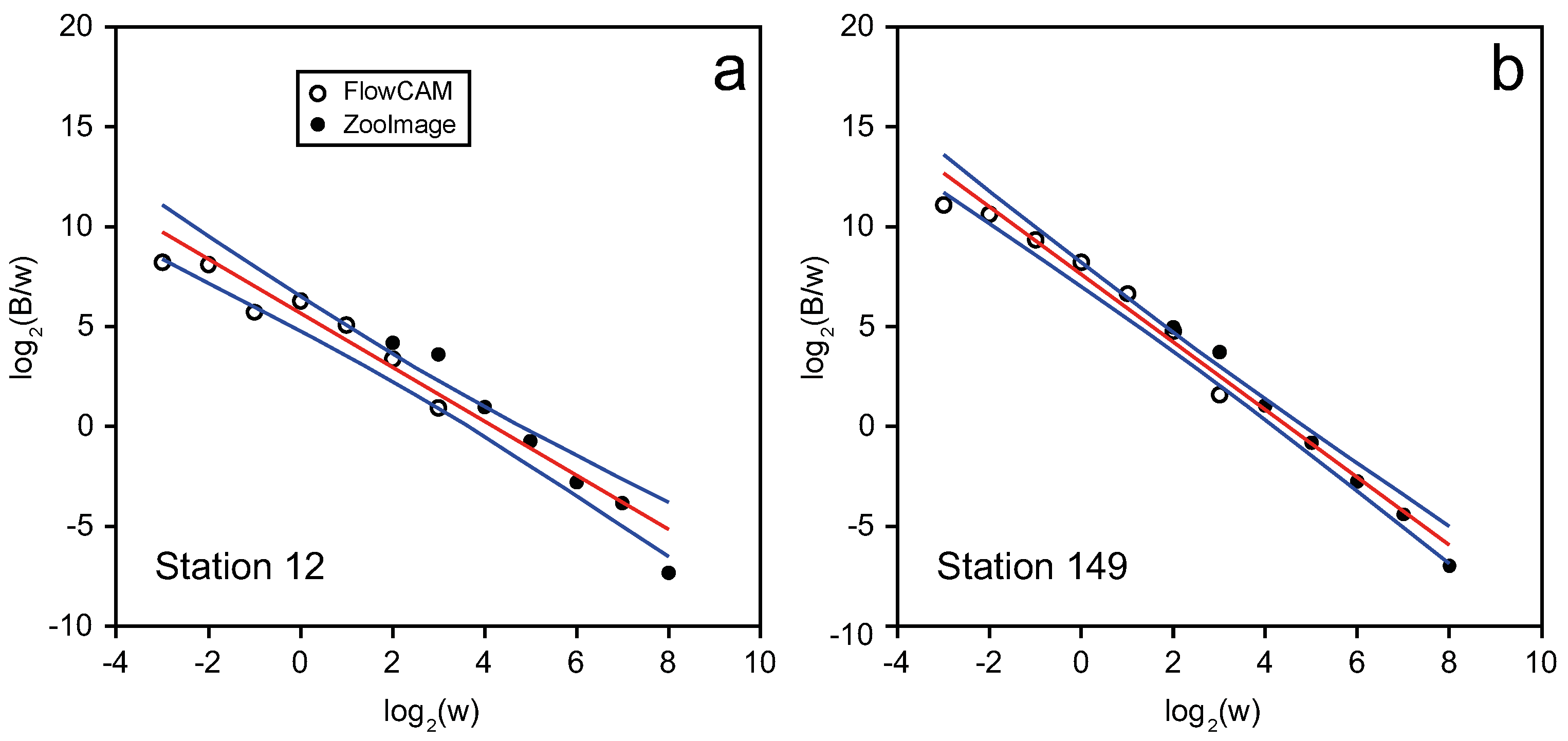
2.3. Abundance Size Spectra
2.4. Statistical Analyses
3. Results
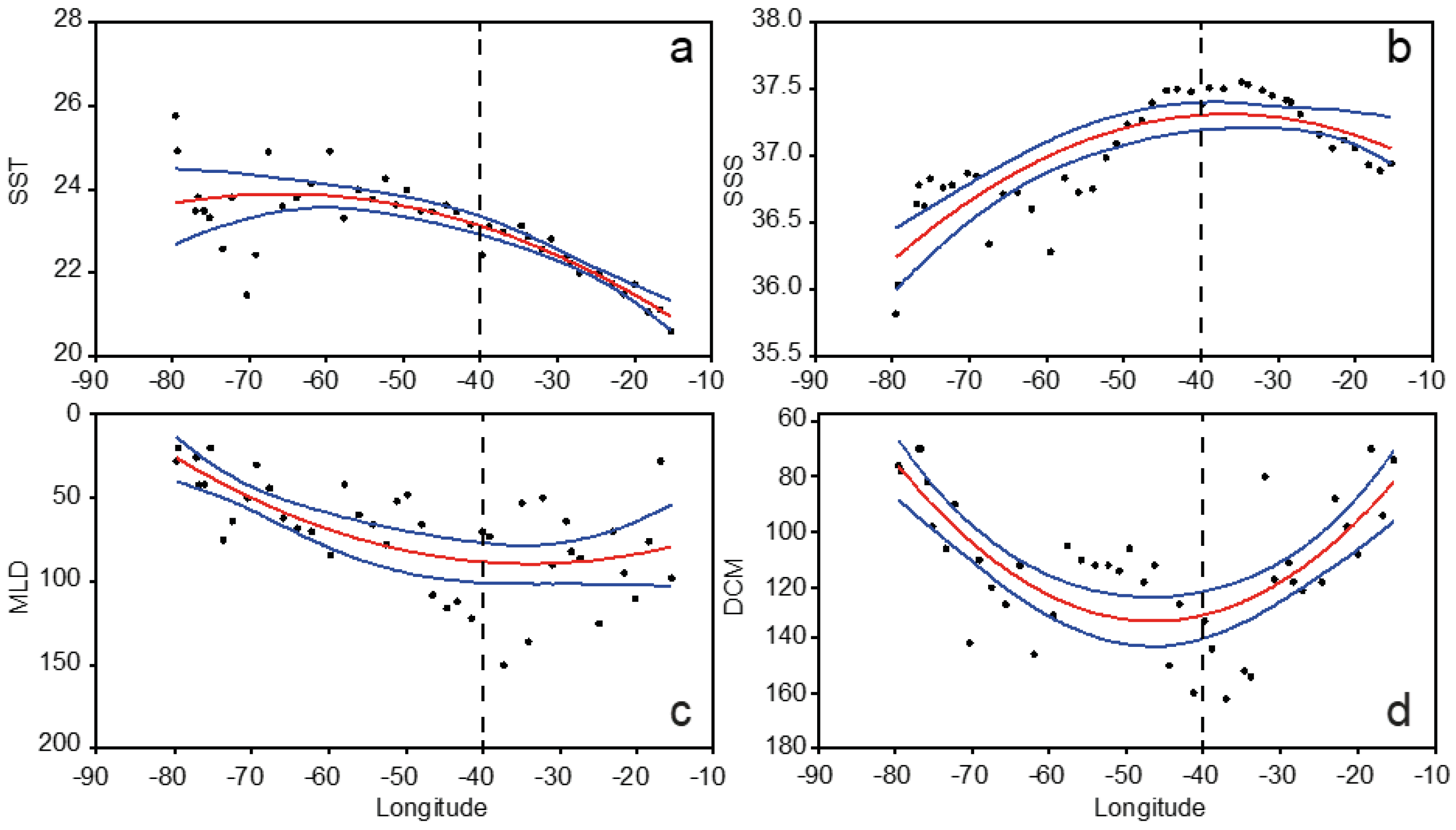
3.1. Hydrography
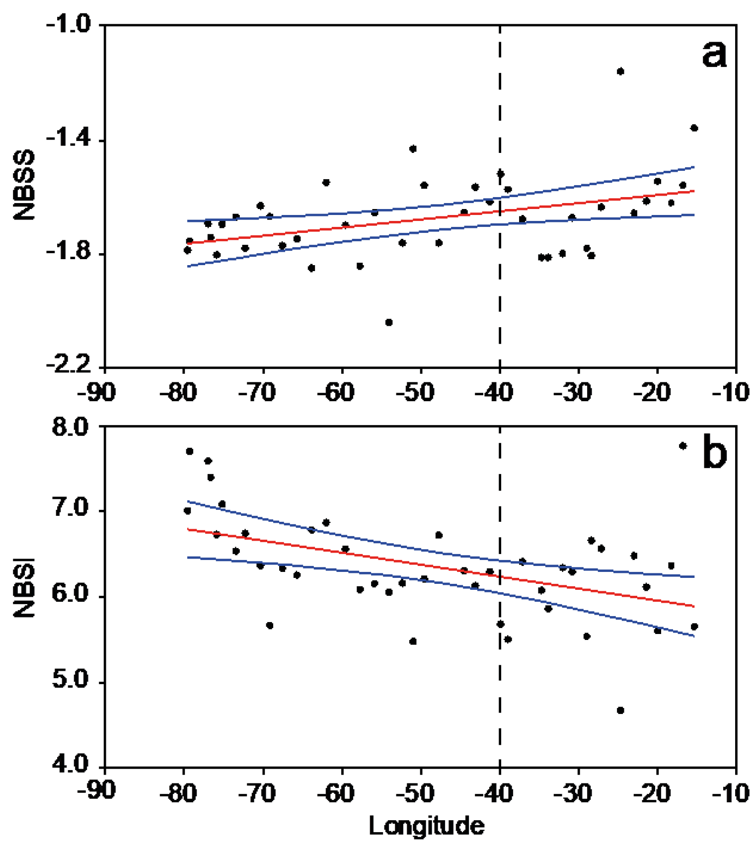
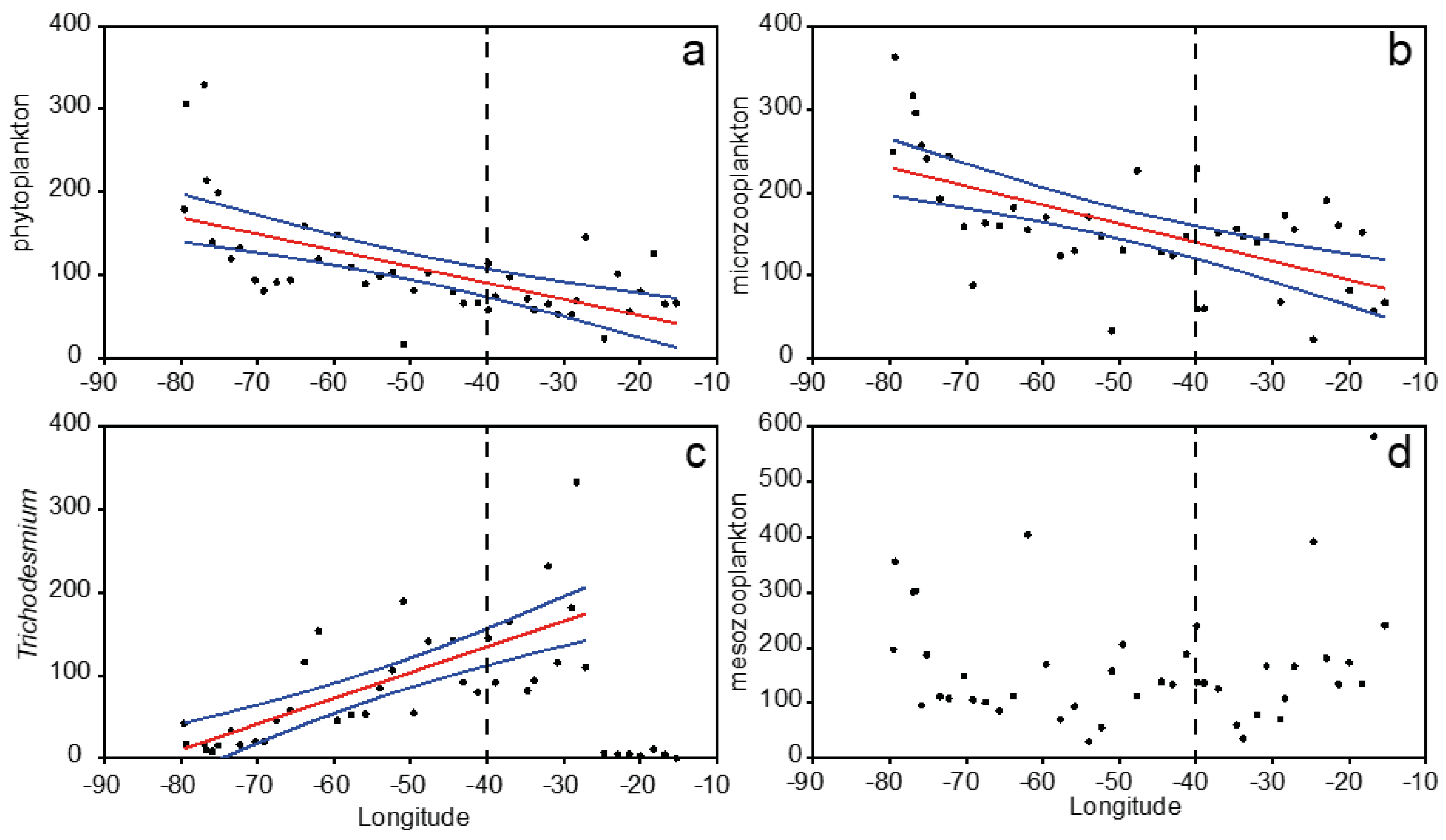
3.2. Plankton Size-Spectra and Abundance
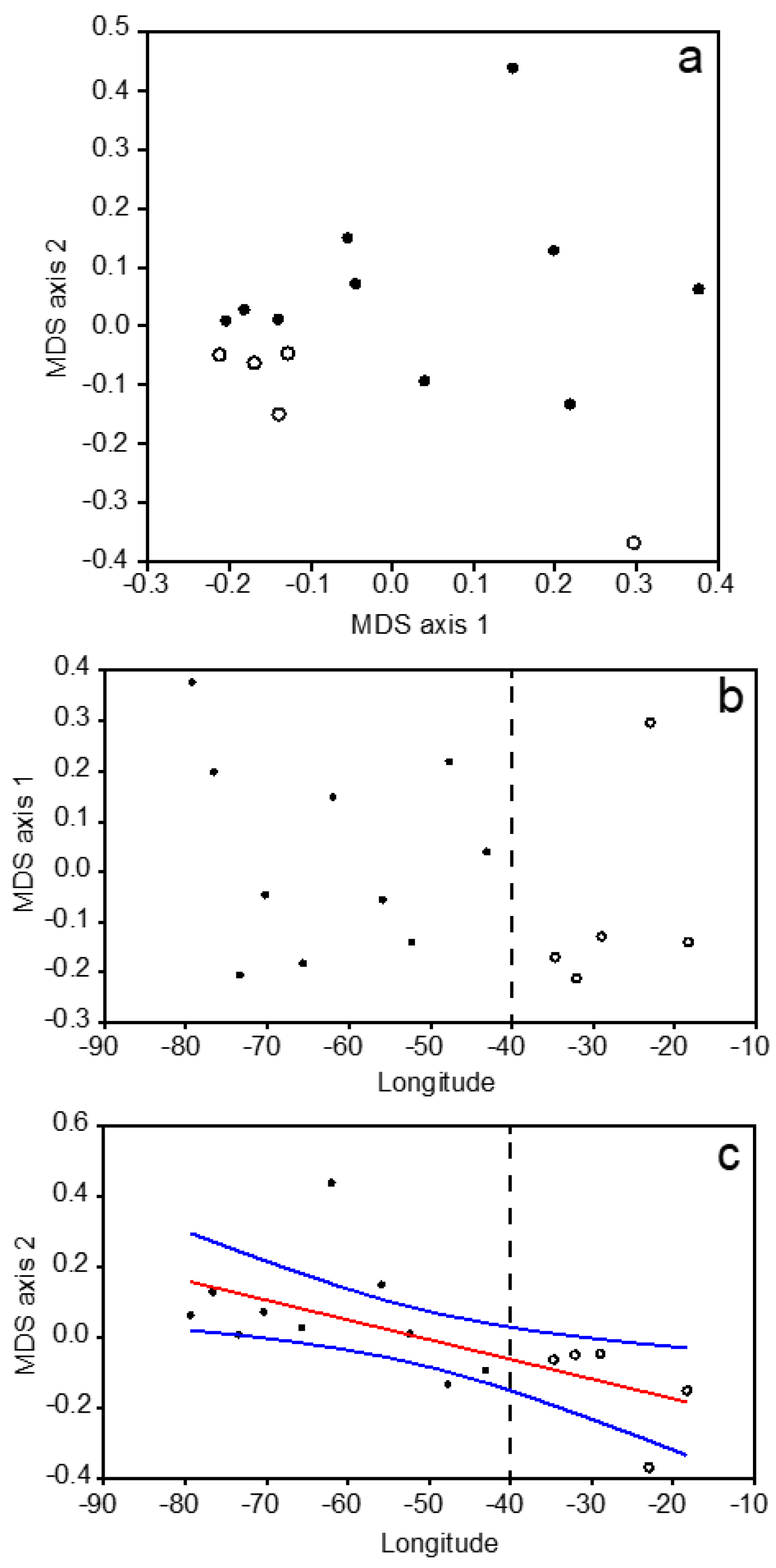
3.3. Mesozooplankton Taxonomic Assemblages
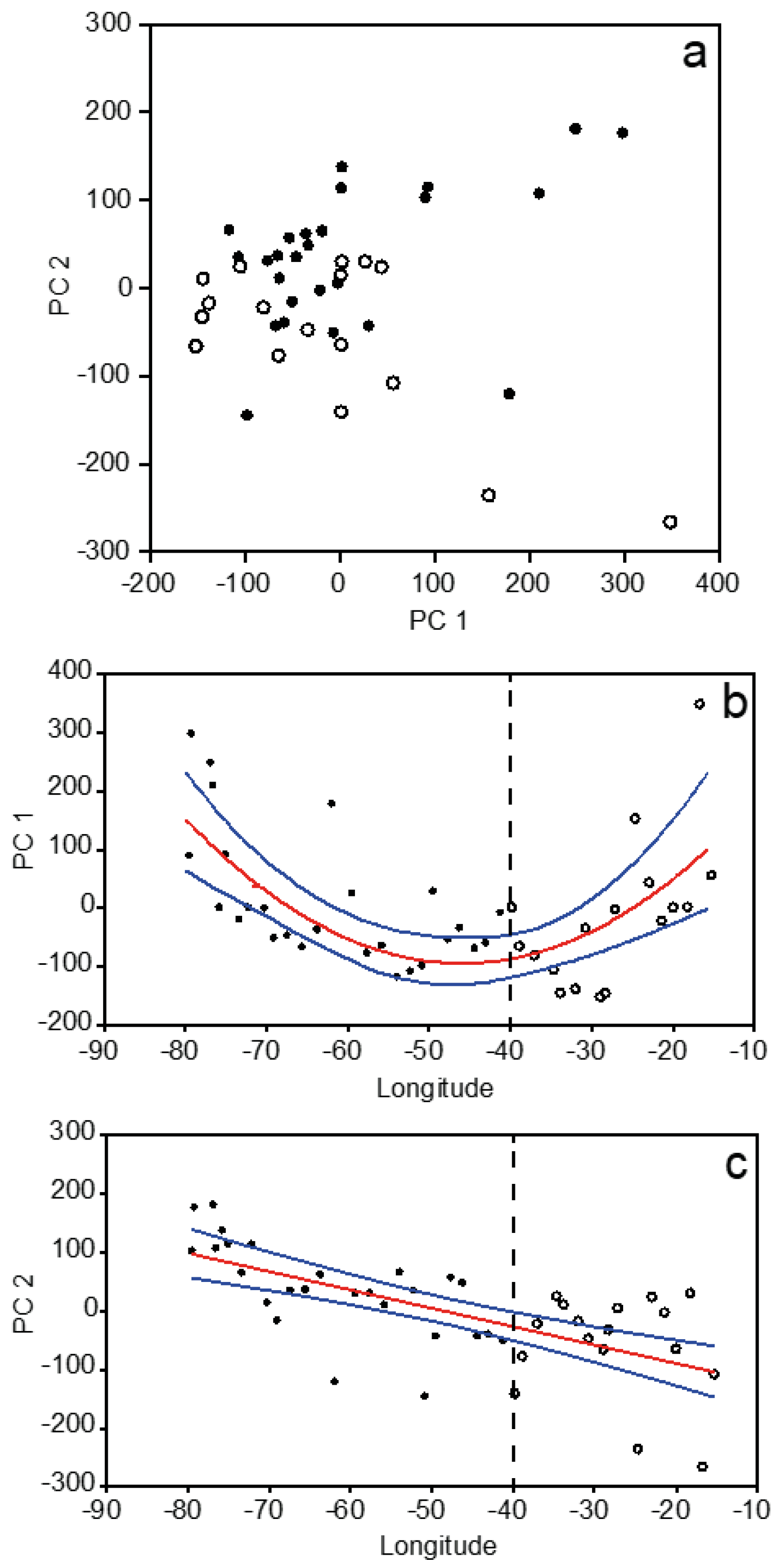
3.4. Overall Zonal Patterns
4. Discussion
4.1. Zonal Variability of the North Atlantic Subtropical Gyre
4.2. Continuous Gradients vs. Discrete Biogeographic Provinces
4.3. Implications for Modelling and Forecasting Subtropical Plankton
5. Conclusions
Supplementary Materials
Author Contributions
Funding
Institutional Review Board Statement
Informed Consent Statement
Data Availability Statement
Acknowledgments
Conflicts of Interest
References
- IPCC. Climate Change 2023: Synthesis Report. In Contribution of Working Groups I, II and III to the Sixth Assessment Report of the Intergovernmental Panel on Climate Change; IPCC: Geneva, Switzerland, 2023; p. 115. [Google Scholar]
- Parrilla, G.; Lavín, A.; Bryden, H.; García, M.; Millard, R. Rising temperatures in the subtropical North Atlantic Ocean over the past 35 years. Nature 1994, 369, 48–51. [Google Scholar] [CrossRef]
- Lavin, A.M.; Bryden, H.L.; Parrilla, G. Mechanisms of heat, freshwater, oxygen and nutrient transports and budgets at 24.5° N in the subtropical North Atlantic. Deep Sea Res. 2003, 50, 1099–1128. [Google Scholar] [CrossRef]
- Bryden, H.L.; Longworth, H.R.; Cunningham, S.A. Slowing of the Atlantic meridional overturning circulation at 25° N. Nature 2005, 438, 655–657. [Google Scholar] [CrossRef] [PubMed]
- Behrenfeld, M.J.; O’Malley, R.T.; Siegel, D.A.; McClain, C.L.; Sarmiento, J.L.; Feldman, G.C.; Milligan, A.J.; Falkowski, P.G.; Letelier, R.M.; Boss, E.S. Climate-driven trends in contemporary ocean productivity. Nature 2006, 444, 752–755. [Google Scholar] [CrossRef] [PubMed]
- Polovina, J.J.; Howell, E.A.; Abecassis, M. Ocean’s least productive waters are expanding. Geophys. Res. Lett. 2008, 35, L03618. [Google Scholar] [CrossRef]
- Signorini, S.R.; Franz, B.A.; McClain, C.R. Chlorophyll variability in the oligotrophic gyres: Mechanisms, seasonality and trends. Front. Mar. Sci. 2015, 2, 1. [Google Scholar] [CrossRef]
- San Martin, E.; Harris, R.P.; Irigoien, X. Latitudinal variation in plankton size spectra in the Atlantic Ocean. Deep Sea Res. II 2006, 53, 1560–1572. [Google Scholar] [CrossRef]
- Armengol, L.; Calbet, A.; Franchy, G.; Rodríguez-Santos, A.; Hernández-León, S. Planktonic food web structure and trophic transfer efficiency along a productivity gradient in the tropical and subtropical Atlantic Ocean. Sci. Rep. 2019, 9, 2044. [Google Scholar] [CrossRef]
- Fernández, A.; Mouriño-Carballido, B.; Bode, A.; Varela, M.; Marañón, E. Latitudinal distribution of Trichodesmium spp. and N2 fixation in the Atlantic Ocean. Biogeosciences 2010, 7, 3167–3176. [Google Scholar] [CrossRef]
- Shao, Z.; Xu, Y.; Wang, H.; Luo, W.; Wang, L.; Huang, Y.; Agawin, N.S.R.; Ahmed, A.; Benavides, M.; Bentzon-Tilia, M.; et al. Global oceanic diazotroph database version 2 and elevated estimate of global oceanic N2 fixation. Earth Syst. Sci. Data 2023, 15, 3673–3709. [Google Scholar] [CrossRef]
- Décima, M. Zooplankton trophic structure and ecosystem productivity. Mar. Ecol. Prog. Ser. 2022, 692, 23–42. [Google Scholar] [CrossRef]
- Longhurst, A.R. Ecological Geography of the Sea, 2nd ed.; Elsevier: Amsterdam, The Netherlands, 2007; p. 542. [Google Scholar]
- Hofmann Elizondo, U.; Righetti, D.; Benedetti, F.; Vogt, M. Biome partitioning of the global ocean based on phytoplankton biogeography. Prog. Oceanogr. 2021, 194, 102530. [Google Scholar] [CrossRef]
- Fernández-Castro, B.; Pahlow, M.; Mouriño-Carballido, B.; Marañón, E.; Oschlies, A. Optimality-based Trichodesmium diazotrophy in the North Atlantic subtropical gyre. J. Plankton Res. 2016, 38, 946–963. [Google Scholar] [CrossRef]
- Pérez, F.F.; Mercier, H.; Vazquez-Rodriguez, M.; Lherminier, P.; Velo, A.; Pardo, P.C.; Roson, G.; Rios, A.F. Atlantic Ocean CO2 uptake reduced by weakening of the meridional overturning circulation. Nat. Geosci. 2013, 6, 146–152. [Google Scholar] [CrossRef]
- Guallart, E.F.; Fajar, N.M.; Padín, X.A.; Vázquez-Rodríguez, M.; Calvo, E.; Ríos, A.F.; Hernández-Guerra, A.; Pelejero, C.; Pérez, F.F. Ocean acidification along the 24.5° N section in the subtropical North Atlantic. Geophys. Res. Lett. 2015, 42, 450–458. [Google Scholar] [CrossRef]
- Marañón, E.; Holligan, P.M.; Varela, M.; Mouriño, B.; Bale, A.J. Basin-scale variability of phytoplankton biomass, production and growth in the Atlantic Ocean. Deep Sea Res. 2000, 47, 825–857. [Google Scholar] [CrossRef]
- Mompeán, C.; Bode, A.; Benítez-Barrios, V.M.; Domínguez-Yanes, J.F.; Escánez, J.; Fraile-Nuez, E. Spatial patterns of plankton biomass and stable isotopes reflect the influence of the nitrogen-fixer Trichodesmium along the subtropical North Atlantic. J. Plankton Res. 2013, 35, 513–525. [Google Scholar] [CrossRef]
- Fernández, A.; Marañón, E.; Bode, A. Large-scale meridional and zonal variability in the nitrogen isotopic composition of plankton in the Atlantic Ocean. J. Plankton Res. 2014, 36, 1060–1073. [Google Scholar] [CrossRef]
- Moreno-Ostos, E.; Blanco, J.M.; Agustí, S.; Lubián, L.M.; Rodríguez, V.; Palomino, R.L.; Llabrés, M.; Rodríguez, J. Phytoplankton biovolume is independent from the slope of the size spectrum in the oligotrophic Atlantic Ocean. J. Mar. Syst. 2015, 152, 42–50. [Google Scholar] [CrossRef]
- Benavides, M.; Moisander, P.H.; Daley, M.C.; Bode, A.; Arístegui, J. Longitudinal variability of diazotroph abundances in the subtropical North Atlantic Ocean. J. Plankton Res. 2016, 38, 662–672. [Google Scholar] [CrossRef]
- Hernández-Guerra, A.; Pelegrí, J.L.; Fraile-Nuez, E.; Benítez-Barrios, V.; Emelianov, M.; Pérez-Hernández, M.D.; Vélez-Belchí, P. Meridional overturning transports at 7.5° N and 24.5° N in the Atlantic Ocean during 1992–1993 and 2010–2011. Prog. Oceanogr. 2014, 128, 98–114. [Google Scholar] [CrossRef]
- Harrison, W.G.; Arístegui, J.; Head, E.J.H.; Li, W.K.W.; Longhurst, A.R.; Sameoto, D.D. Basin-scale variability in plankton biomass and community metabolism in the sub-tropical North Atlantic Ocean. Deep Sea Res. II 2001, 48, 2241–2270. [Google Scholar] [CrossRef]
- Fernández, A.; Graña, R.; Mouriño-Carballido, B.; Bode, A.; Varela, M.; Domínguez, J.F.; Escánez, J.; de Armas, D.; Marañón, E. Community N2 fixation and Trichodesmium spp. abundance along longitudinal gradients in the eastern subtropical North Atlantic. ICES J. Mar. Sci. 2013, 70, 223–231. [Google Scholar] [CrossRef]
- Grasshoff, K.; Ehrhardt, M.; Kremling, K. Methods of Seawater Analysis, 2nd. ed.; Verlag Chemie: Weinheim, Germany, 1983; p. 419. [Google Scholar]
- de Boyer Montégut, C.; Madec, G.; Fischer, A.S.; Lazar, A.; Iudicone, D. Mixed layer depth over the global ocean: An examination of profile data and a profile-based climatology. J. Geophys. Res. C Ocean. 2004, 109, C12003. [Google Scholar] [CrossRef]
- Pérez, F.F.; Hernández Guerra, A. CTD Data from Cruise 29AH20110128, Exchange Version. 2015. Available online: https://cchdo.ucsd.edu/cruise/29AH20110128 (accessed on 1 June 2015).
- Mompeán, C.; Bode, A.; Gier, E.; McCarthy, M.D. Bulk vs. aminoacid stable N isotope estimations of metabolic status and contributions of nitrogen fixation to size-fractionated zooplankton biomass in the subtropical N Atlantic. Deep Sea Res. 2016, 114, 137–148. [Google Scholar] [CrossRef]
- Álvarez, E.; Moyano, M.; López-Urrutia, A.; Nogueira, E.; Scharek, R. Routine determination of plankton community composition and size structure: A comparison between FlowCAM and light microscopy. J. Plankton Res. 2014, 36, 170–184. [Google Scholar] [CrossRef]
- Fluid Imaging Technologies. FlowCAM® Manual. Version 3.2; Fluid Imaging Technologies Inc.: Yarmouth, MA, USA, 2012; 162p, Available online: https://www.fluidimaging.com/ (accessed on 20 June 2014).
- Bachiller, E.; Fernandes, J.A. Zooplankton image analysis manual: Automated identification by means of scanner and digital camera as imaging devices. Rev. Investig. Mar. 2011, 18, 17–37. [Google Scholar]
- WoRMS Editorial Board. World Register of Marine Species. 2023. Available online: https://www.marinespecies.org (accessed on 22 September 2023).
- Shao, Z.; Xu, Y.; Wang, H.; Luo, W.; Wang, L.; Huang, Y.; Luo, Y.-W. Version 2 of the Global Oceanic Diazotroph Database. 2022. Available online: https://figshare.com/ndownloader/articles/21677687/versions/3 (accessed on 26 February 2024).
- Platt, T.; Denman, K. The structure of pelagic marine ecosystems. Rapp. P.-V. Réun. Cons. Int. Explor. Mer. 1978, 173, 60–65. [Google Scholar]
- Blanco, J.M.; Echevarria, F.; Garcia, C.M. Dealing with size spectra: Some conceptual and mathematical problems. Sci. Mar. (Barc.) 1994, 58, 17–29. [Google Scholar]
- Working, H.; Hotelling, H. Applications of the theory of error to the interpretation of trends. J. Am. Stat. Assoc. 1929, 24, 73–85. [Google Scholar] [CrossRef]
- Magurran, A.E. Measuring Biological Diversity; Blackwell Science Ltd.: Oxford, UK, 2004; p. 215. [Google Scholar]
- Hammer, Ø.; Harper, D.A.T.; Ryan, P.D. PAST: Paleontological Statistics Software Package for Education and Data Analysis. Palaeontologia Electronica. 2001. Available online: https://palaeo-electronica.org/2001_1/past/issue1_01.htm (accessed on 6 March 2020).
- Mouriño-Carballido, B.; Neuer, S.C. Regional differences in the role of eddy pumping in the North Atlantic subtropical gyre. Oceanography 2008, 21, 52–61. [Google Scholar] [CrossRef]
- Smith, R.D.; Maltrud, M.E.; Bryan, F.O.; Hecht, M.W. Numerical simulation of the North Atlantic Ocean at 1/10°. J. Phys. Oceanogr. 2000, 30, 1532–1561. [Google Scholar] [CrossRef]
- McGillicuddy, D.J.; Anderson, L.A.; Bates, N.R.; Bibby, T.; Buesseler, K.O.; Carlson, C.A.; Davis, C.S.; Ewart, C.; Falkowski, P.G.; Goldthwait, S.A.; et al. Eddy/wind interactions stimulate extraordinary mid-ocean plankton blooms. Science 2007, 316, 1021–1026. [Google Scholar] [CrossRef]
- Cianca, A.; Helmke, P.; Mouriño, B.; Rueda, M.J.; Llinás, O.; Neuer, S. Decadal analysis of hydrography and in situ nutrient budgets in the western and eastern North Atlantic subtropical gyre. J. Geophys. Res. C Ocean. 2007, 112, C07025. [Google Scholar] [CrossRef]
- Pelegrí, J.L.; Arístegui, J.; Cana, L.; González-Dávila, M.; Hernández-Guerra, A.; Hernández-León, S.; Marrero-Díaz, A.; Montero, M.F.; Sangrá, P.; Santana-Casiano, M. Coupling between the open ocean and the coastal upwelling region off northwest Africa: Water recirculation and offshore pumping of organic matter. J. Mar. Syst. 2005, 54, 3–37. [Google Scholar] [CrossRef]
- Capone, D.G.; Burns, J.A.; Montoya, J.P.; Subramaniam, A.; Mahaffey, C.; Gunderson, T.; Michaels, A.F.; Carpenter, E.J. Nitrogen fixation by Trichodesmium spp.: An important source of new nitrogen to the tropical and subtropical North Atlantic Ocean. Glob. Biogeochem. Cycles 2005, 19, GB2024. [Google Scholar] [CrossRef]
- Olson, E.M.; McGillicuddy, D.J.J.; Dyhrman, S.T.; Waterbury, J.B.; Davis, C.S.; Solow, A.R. The depth-distribution of nitrogen fixation by Trichodesmium spp. colonies in the tropical–subtropical North Atlantic. Deep Sea Res. 2015, 104, 72–91. [Google Scholar] [CrossRef]
- Schmitz Jr, W.J.; Richardson, P.L. On the sources of the Florida Current. Deep Sea Res. 1991, 38, S379–S409. [Google Scholar] [CrossRef]
- Devred, E.; Sathyendranath, S.; Platt, T. Delineation of ecological provinces using ocean colour radiometry. Mar. Ecol. Prog. Ser. 2007, 346, 07149. [Google Scholar] [CrossRef]
- Kavanaugh, M.T.; Hales, B.; Saraceno, M.; Spitz, Y.H.; White, A.E.; Letelier, R.M. Hierarchical and dynamic seascapes: A quantitative framework for scaling pelagic biogeochemistry and ecology. Prog. Oceanogr. 2014, 120, 291–304. [Google Scholar] [CrossRef]
- Foster, D.; Gagne, D.J.; Whitt, D.B. Probabilistic machine learning estimation of ocean mixed layer depth from dense satellite and sparse in situ observations. J. Adv. Model. Earth Syst. 2021, 13, e2021MS002474. [Google Scholar] [CrossRef]
- Druon, J.-N.; Hëlaouét, P.; Beaugrand, G.; Fromentin, J.-M.; Palialexis, A.; Hoepffner, N. Satellite-based indicator of zooplankton distribution for global monitoring. Sci. Rep. 2021, 9, 4732. [Google Scholar] [CrossRef] [PubMed]
- Beaugrand, G. Theoretical basis for predicting climate-induced abrupt shifts in the oceans. Phil. Trans. R. Soc. B 2015, 370, 20130264. [Google Scholar] [CrossRef]
- Kléparski, L.; Beaugrand, G.; Kirby, R.R. How do plankton species coexist in an apparently unstructured environment? Biol. Lett. 2022, 18, 20220207. [Google Scholar] [CrossRef] [PubMed]
- Acevedo-Trejos, E.; Brandt, G.; Bruggeman, J.; Merico, A. Mechanisms shaping size structure and functional diversity of phytoplankton communities in the ocean. Sci. Rep. 2015, 5, 08918. [Google Scholar] [CrossRef] [PubMed]
- González-García, C.; Agustí, S.; Aiken, J.; Bertrand, A.; Bittencourt Farias, G.; Bode, A.; Carré, C.; Gonçalves-Araujo, R.; Harbour, D.S.; Huete-Ortega, M.; et al. Basin-scale variability in phytoplankton size-abundance spectra across the Atlantic Ocean. Prog. Oceanogr. 2023, 217, 103104. [Google Scholar] [CrossRef]
- Quiñones, R.A.; Platt, T.; Rodríguez, J. Patterns of biomass-size spectra from oligotrophic waters of the Northwest Atlantic. Prog. Oceanogr. 2003, 57, 405–427. [Google Scholar] [CrossRef]
- Zhou, M. What determines the slope of a plankton biomass spectrum? J. Plankton Res. 2006, 28, 437–448. [Google Scholar] [CrossRef]
- Rayner, D.; Hirschi, J.J.M.; Kanzow, T.; Johns, W.E.; Wright, P.G.; Frajka-Williams, E.; Bryden, H.L.; Meinen, C.S.; Baringer, M.O.; Marotzke, J.; et al. Monitoring the Atlantic meridional overturning circulation. Deep Sea Res. II 2011, 58, 1744–1753. [Google Scholar] [CrossRef]
- Lozier, M.S. Overturning in the North Atlantic. Ann. Rev. Mar. Sci. 2012, 4, 291–315. [Google Scholar] [CrossRef]
- Sathyendranath, S.; Longhurst, A.; Caverhill, C.M.; Platt, T. Regionally and seasonally differentiated primary production in the North Atlantic. Deep Sea Res. 1995, 42, 1773–1802. [Google Scholar] [CrossRef]
- McClain, C.R.; Signorini, S.R.; Christian, J.R. Subtropical gyre variability observed by ocean-color satellites. Deep Sea Res. II 2004, 51, 281–301. [Google Scholar] [CrossRef]
- Siemer, J.P.; Machín, F.; González-Vega, A.; Arrieta, J.M.; Gutiérrez-Guerra, M.A.; Pérez-Hernández, M.D.; Vélez-Belchí, P.; Hernández-Guerra, A.; Fraile-Nuez, E. Recent trends in SST, Chl-a, productivity and wind stress in upwelling and open ocean areas in the upper Eastern North Atlantic subtropical gyre. J. Geophys. Res. C Ocean. 2021, 126, e2021JC017268. [Google Scholar] [CrossRef]
- Armengol, L.; Franchy, G.; Ojeda, A.; Hernández-León, S. Plankton community changes from warm to cold winters in the oligotrophic subtropical ocean. Front. Mar. Sci. 2020, 7, 677. [Google Scholar] [CrossRef]
- Couret, M.; Landeira, J.M.; Santana del Pino, Á.; Hernández-León, S. A 50-year (1971–2021) mesozooplankton biomass data collection in the Canary Current System: Base line, gaps, trends, and future prospect. Prog. Oceanogr. 2023, 216, 103073. [Google Scholar] [CrossRef]
- Steinberg, D.K.; Lomas, M.W.; Cope, J.S. Long-term increase in mesozooplankton biomass in the Sargasso Sea: Linkage to climate and implications for food web dynamics and biogeochemical cycling. Glob. Biogeochem. Cycles 2012, 26, GB1004. [Google Scholar] [CrossRef]
- Ivory, J.A.; Steinberg, D.K.; Latour, R.J. Diel, seasonal, and interannual patterns in mesozooplankton abundance in the Sargasso Sea. ICES J. Mar. Sci. 2019, 76, 217–231. [Google Scholar] [CrossRef]


| NASW | NASE | ||
|---|---|---|---|
| Variable | Mean ± SD (n) | Mean ± SD (n) | p |
| SST | 23.63 ± 0.76 (25) | 22.13 ± 0.76 (17) | 0.000 |
| SSS | 36.86 ± 0.38 (25) | 37.28 ± 0.24 (17) | 0.000 |
| SFluor | 0.11 ± 0.04 (25) | 0.20 ± 0.13 (17) | 0.014 |
| DCM | 113.88 ± 22.76 (25) | 115.71 ± 27.52 (17) | 0.816 |
| MLD | 75.72 ± 25.25 (25) | 97.12 ± 27.78 (17) | 0.013 |
| MLO2 | 4.83 ± 0.07 (24) | 4.89 ± 0.08 (17) | 0.029 |
| MLNO3 | 0.13 ± 0.08 (17) | 0.21 ± 0.22 (16) | 0.178 |
| MLSiO2 | 0.30 ± 0.33 (17) | 0.73 ± 0.17 (16) | 0.000 |
| MLPO4 | 0.35 ± 0.27 (17) | 0.57 ± 0.14 (16) | 0.007 |
| MLFluor | 0.13 ± 0.05 (25) | 0.20 ± 0.09 (17) | 0.003 |
| NBSS | −2.71 ± 0.12 (25) | −2.62 ± 0.17 (17) | 0.066 |
| NBSI | 6.53 ± 0.55 (25) | 6.10 ± 0.67 (17) | 0.025 |
| Tricho | 59.84 ± 46.56 (25) | 81.00 ± 83.69 (17) | 0.300 |
| phyto | 128.38 ± 70.48 (26) | 74.37 ± 29.37 (17) | 0.001 |
| microz | 185.92 ± 73.83 (26) | 147.95 ± 121.24 (17) | 0.208 |
| mesoz | 156.46 ± 93.45 (25) | 178.04 ± 133.63 (17) | 0.541 |
| Cope | 175.34 ± 187.66 (9) | 112.82 ± 132.09 (6) | 0.494 |
| Tuni | 35.50 ± 35.07 (9) | 23.57 ± 23.74 (6) | 0.481 |
| Cnid | 4.43 ± 3.18 (9) | 5.53 ± 5.87 (6) | 0.644 |
| Other | 29.56 ± 22.23 (9) | 23.28 ± 31.62 (6) | 0.657 |
| Species/Group | MDS 1 | Species/Group | MDS 2 |
|---|---|---|---|
| Calanoida (other) | 0.911 | Oithona plumífera | 0.533 |
| Oncaea spp. | 0.495 | Oithona spp. | 0.220 |
| Conchoecia spp. | 0.484 | Foraminifera | 0.176 |
| Lucicutia spp. | 0.317 | Haloptilus sp. | 0.099 |
| Calocalanus spp. | 0.207 | Lubbockia sp. | 0.091 |
| Lubbockia sp. | −0.154 | Acartia negligens | −0.105 |
| Euphausiacea | −0.170 | Oncaea spp. | −0.158 |
| Decapoda (larvae) | −0.278 | Acartia spp. | −0.225 |
| Paracalanus spp. | −0.356 | Calanoida (other) | −0.298 |
| Mesocalanus tenuicornis | −0.453 | Haloptilus longicornis | −0.302 |
| Long | SST | SSS | SFluor | DCM | MLD | NBSS | NBSI | Tricho | Phyto | Microz | Mesoz | Cope | Tuni | Cnid | Other | |
|---|---|---|---|---|---|---|---|---|---|---|---|---|---|---|---|---|
| Long | 0.000 | 0.000 | 0.001 | 0.303 | 0.000 | 0.010 | 0.003 | 0.144 | 0.000 | 0.000 | 0.695 | 0.330 | 0.205 | 0.617 | 0.444 | |
| SST | −0.710 | 0.001 | 0.000 | 0.676 | 0.073 | 0.005 | 0.047 | 0.582 | 0.005 | 0.001 | 0.394 | 0.127 | 0.115 | 0.499 | 0.469 | |
| SSS | 0.661 | −0.485 | 0.270 | 0.001 | 0.000 | 0.206 | 0.001 | 0.001 | 0.000 | 0.001 | 0.113 | 0.020 | 0.060 | 0.155 | 0.078 | |
| SFluor | 0.498 | −0.521 | 0.172 | 0.033 | 0.506 | 0.166 | 0.625 | 0.531 | 0.707 | 0.321 | 0.521 | 0.464 | 0.364 | 0.060 | 0.457 | |
| DCM | 0.161 | 0.066 | 0.491 | −0.326 | 0.000 | 0.711 | 0.012 | 0.009 | 0.001 | 0.007 | 0.146 | 0.559 | 0.556 | 0.020 | 0.292 | |
| MLD | 0.559 | −0.276 | 0.585 | 0.104 | 0.551 | 0.043 | 0.001 | 0.112 | 0.001 | 0.017 | 0.247 | 0.314 | 0.484 | 0.726 | 0.432 | |
| NBSS | 0.393 | −0.424 | 0.199 | 0.218 | 0.059 | 0.314 | 0.007 | 0.226 | 0.031 | 0.000 | 0.000 | 0.215 | 0.140 | 0.136 | 0.230 | |
| NBSI | −0.453 | 0.308 | −0.478 | −0.078 | −0.383 | −0.496 | −0.413 | 0.370 | 0.000 | 0.000 | 0.014 | 0.004 | 0.004 | 0.061 | 0.012 | |
| Tricho | 0.227 | 0.086 | 0.499 | −0.098 | 0.396 | 0.246 | −0.191 | −0.142 | 0.032 | 0.201 | 0.067 | 0.425 | 0.434 | 0.012 | 0.124 | |
| phyto | −0.628 | 0.417 | −0.607 | −0.059 | −0.480 | −0.483 | −0.333 | 0.749 | −0.328 | 0.000 | 0.119 | 0.009 | 0.016 | 0.047 | 0.031 | |
| microz | −0.626 | 0.474 | −0.483 | −0.155 | −0.403 | −0.362 | −0.545 | 0.779 | −0.199 | 0.845 | 0.999 | 0.024 | 0.039 | 0.090 | 0.028 | |
| mesoz | 0.062 | −0.133 | −0.245 | 0.101 | −0.225 | −0.180 | 0.548 | 0.377 | −0.282 | 0.241 | 0.000 | 0.000 | 0.000 | 0.050 | 0.001 | |
| Cope | −0.270 | 0.412 | −0.592 | −0.205 | −0.164 | −0.279 | 0.340 | 0.699 | −0.223 | 0.648 | 0.578 | 0.892 | 0.000 | 0.025 | 0.000 | |
| Tuni | −0.347 | 0.424 | −0.496 | −0.253 | −0.165 | −0.196 | 0.400 | 0.690 | −0.218 | 0.609 | 0.538 | 0.924 | 0.928 | 0.035 | 0.000 | |
| Cnid | 0.141 | −0.189 | −0.386 | 0.496 | −0.593 | −0.099 | 0.403 | 0.494 | −0.630 | 0.521 | 0.452 | 0.514 | 0.575 | 0.547 | 0.005 | |
| Other | −0.214 | 0.203 | −0.469 | −0.208 | −0.291 | −0.220 | 0.330 | 0.631 | −0.415 | 0.558 | 0.565 | 0.756 | 0.881 | 0.883 | 0.684 |
| Variable | PC 1 | PC 2 |
|---|---|---|
| Longitude | −0.037 | −0.139 |
| SST | 0.000 | 0.006 |
| SSS | −0.002 | −0.002 |
| SFluor | 0.000 | 0.000 |
| DCM | −0.093 | −0.094 |
| MLD | −0.102 | −0.122 |
| NBSS | 0.000 | −0.001 |
| NBSI | 0.003 | 0.003 |
| Trichodesmium | −0.334 | −0.174 |
| Phytoplankton | 0.312 | 0.499 |
| Microzooplankton | 0.218 | 0.684 |
| Mesozooplankton | 0.851 | −0.458 |
Disclaimer/Publisher’s Note: The statements, opinions and data contained in all publications are solely those of the individual author(s) and contributor(s) and not of MDPI and/or the editor(s). MDPI and/or the editor(s) disclaim responsibility for any injury to people or property resulting from any ideas, methods, instructions or products referred to in the content. |
© 2024 by the authors. Licensee MDPI, Basel, Switzerland. This article is an open access article distributed under the terms and conditions of the Creative Commons Attribution (CC BY) license (https://creativecommons.org/licenses/by/4.0/).
Share and Cite
Bode, A.; Louro, M.Á.; Rey, E.; Lamas, A.F. Continuous Zonal Gradients Characterize Epipelagic Plankton Assemblages and Hydrography in the Subtropical North Atlantic. Oceans 2024, 5, 109-126. https://doi.org/10.3390/oceans5010007
Bode A, Louro MÁ, Rey E, Lamas AF. Continuous Zonal Gradients Characterize Epipelagic Plankton Assemblages and Hydrography in the Subtropical North Atlantic. Oceans. 2024; 5(1):109-126. https://doi.org/10.3390/oceans5010007
Chicago/Turabian StyleBode, Antonio, María Ángeles Louro, Elena Rey, and Angel F. Lamas. 2024. "Continuous Zonal Gradients Characterize Epipelagic Plankton Assemblages and Hydrography in the Subtropical North Atlantic" Oceans 5, no. 1: 109-126. https://doi.org/10.3390/oceans5010007
APA StyleBode, A., Louro, M. Á., Rey, E., & Lamas, A. F. (2024). Continuous Zonal Gradients Characterize Epipelagic Plankton Assemblages and Hydrography in the Subtropical North Atlantic. Oceans, 5(1), 109-126. https://doi.org/10.3390/oceans5010007