Efficient Encoding of the Traveling Salesperson Problem on a Quantum Computer

Abstract

We propose an amplitude encoding of the traveling salesperson problem along with a method for calculating the cost function using a probability distribution obtained on a quantum computer. Our encoding requires a number of qubits that grows logarithmically with the number of cities. We propose to calculate the cost function using a nonlinear function of expectation values of quantum operators. This is in contrast to the typical method of evaluating the cost function by summing expectation values of quantum operators. We demonstrate our method using a variational quantum eigensolver algorithm to find the shortest route for a given graph. We find that there is a broad range in the hyperparameters of the optimization procedure for which the best route is found.

1. Introduction

The traveling salesperson problem (TSP) is a famous computationally difficult problem in mathematics. The TSP involves a salesperson who wants to visit a number of cities to sell their goods. The salesperson knows the distance to each city and wants to make a travel itinerary that passes through each city following the shortest possible route. While the problem might appear simple, it is theorized to be in the complexity class of NP-hard problems. The challenge is that the number of possible routes grows as $N_C!$ where $N_C$ is the number of cities. Thus, the brute force method of calculating the distance of each route is intractable on a classical computer for even a relatively small set of cities. Many classical algorithms have been developed that approximately solve the TSP, such as branch and bound techniques [1,2,3,4] and other heuristic algorithms [5,6,7,8,9,10,11]; however, there is no known classical algorithm that solves the general TSP exactly with polynomial resources.

Quantum computing may provide improved algorithms for solving the TSP. Imagine a salesperson who can traverse each of the $N_C!$ routes simultaneously. If the salesperson also has a method for finding which of the simultaneously traveled routes is shortest then they could find the shortest route in a single check. This is similar to how a quantum computer operates. A quantum computer can be in a superposition of exponentially many states. If the routes of the TSP are somehow encoded onto the states of a quantum computer, then the quantum computer can simulate our salesperson who can travel all routes simultaneously. The question is, how do we use the quantum computer to find which of the simultaneously traveled routes is shortest?

If we want the quantum computer to return the distance of each route, we would have to take exponentially many measurements of the quantum computer. Therefore, we need a cost function that evaluates a metric for a given quantum superposition that (1) is minimized when the quantum computer is in the state that represents the shortest route and (2) is efficient in the number of required quantum measurements. A typical solution is to derive an operator whose expectation value is minimized for the quantum state that represents the shortest route. This method has been used in a variety of quantum computing algorithms.

There are many quantum algorithms that promise increased efficiency over corresponding classical algorithms. One such algorithm is Grover’s algorithm [12], which offers a polynomial speedup for database search problems. Grover’s algorithm was the first to be proposed as a quadratic speed up over classical algorithms for solving the TSP [13,14,15]. However, these algorithms only work when certain conditions are satisfied. Another quantum algorithm is the Quantum Phase Estimation (QPE) algorithm [16], which has been proposed as an addition to Grover’s algorithm in order to generalize to any TSP [17]. However, the QPE algorithm requires substantial quantum resources, far beyond those currently available. Similarly, the Quantum Adiabatic Algorithm (QAA) [18,19,20,21,22] requires a large amount of quantum resources but may exponentially outperform classical algorithms for solving the TSP. Quantum Annealing [23,24] has also been considered for solving the TSP [25,26,27,28]. While Quantum Annealing has the advantage that it does not require a universal quantum computer, it can be difficult to make precise statements about the efficiency. More contemporary algorithms include the Variational Quantum Eigensolver (VQE) [29,30,31,32] and the Quantum Approximate Optimization Algorithm (QAOA) [33]. Both VQE and QAOA are variational algorithms and both require less resources than QPE or QAA while still providing exponential improvements over classical algorithms for certain problems [31,33]. VQE and QAOA may be tractable on currently available quantum computers and are potentially more efficient at solving the TSP for certain classes of problems [34,35]. We focus on the VQE algorithm in this paper.

A critical part of all quantum algorithms is the encoding. We need an encoding that maps the TSP onto the quantum computer. To the best of our knowledge, the TSP has been exclusively encoded using basis encodings [17,35]. In a basis encoding, possible solutions of a given problem are mapped onto the basis states of the quantum register. For the TSP, for example, each route is mapped onto a basis state. An alternative to basis encoding is amplitude encoding [36]. In an amplitude encoding, the solutions are mapped onto linear combinations of basis states such that the amplitude of each basis state provides information about the solution. Amplitude encodings tend to require fewer qubits than basis encodings. However, for amplitude encoding, it can be difficult to derive a cost operator that can be efficiently implemented on a quantum computer. The process of converting a cost function to a cost operator is not trivial and there is no guarantee that it can be accomplished without exponential resources.

In this work, we present an amplitude encoding for the TSP along with a method to calculate the cost function. Our unique approach to calculating the cost function does not require the construction of a cost operator but instead evaluates the cost based on the probability distribution collected from measurements of the quantum computer. Our method for calculating the cost function allows us to use an amplitude encoding, which exponentially reduces the required number of qubits as compared to basis encodings. Because there is no efficient classical method for reproducing the probability distributions found using the quantum computer, our method may provide an advantage over classical TSP solvers. We demonstrate our method on a state vector simulator for a few small graphs and show that convergence can be found without fine tuning the hyperparameters of the method.

2. Method

2.1. Statement of the TSP

Let us formally define the TSP. We have a number of cities $N_C$ each with a unique label $C_i$ for $i\in \{1,2,\dots N_C\}$. Each pair of cities $C_i$ and $C_j$ is assigned a distance $d_{ij}$. We can define a graph $G=(V,E)$ where the vertices V correspond to the cities and the edges E correspond to the paths between the cities. There are at most $N_E=N_C^2-N_C$ edges for directed graphs and $N_E=(N_C^2-N_C)/2$ edges for undirected graphs. For our demonstration we confine ourselves to undirected graphs; however, we formalize the algorithm for the general case.

A route R is an ordered list of cities, e.g., $R=(C_3,C_2,C_4,C_1)$, that defines the cities that the salesman visits and the order in which each city is visited. Let $\mathrm{idx}\left(R_k\right)$ be the index of the $k^{\mathrm{th}}$ city in R. We define the distance of a route $D\left(R\right)$ as

$$D\left(R\right)=\sum _k{d}_{\mathrm{idx}\left(R_k\right),\mathrm{idx}\left(R_{k+1}\right)},$$

(1)

which is a function that maps routes to real numbers. A route represents a full tour if it contains every city exactly once. Solutions of the TSP are full tours.

2.2. Quantum Amplitude Encoding for the TSP

We now set up the problem for a quantum computer. We use an amplitude encoding to map the TSP routes to states of the quantum computer. This encoding saves resources as compared to basis encodings and is a major advantage of our method.

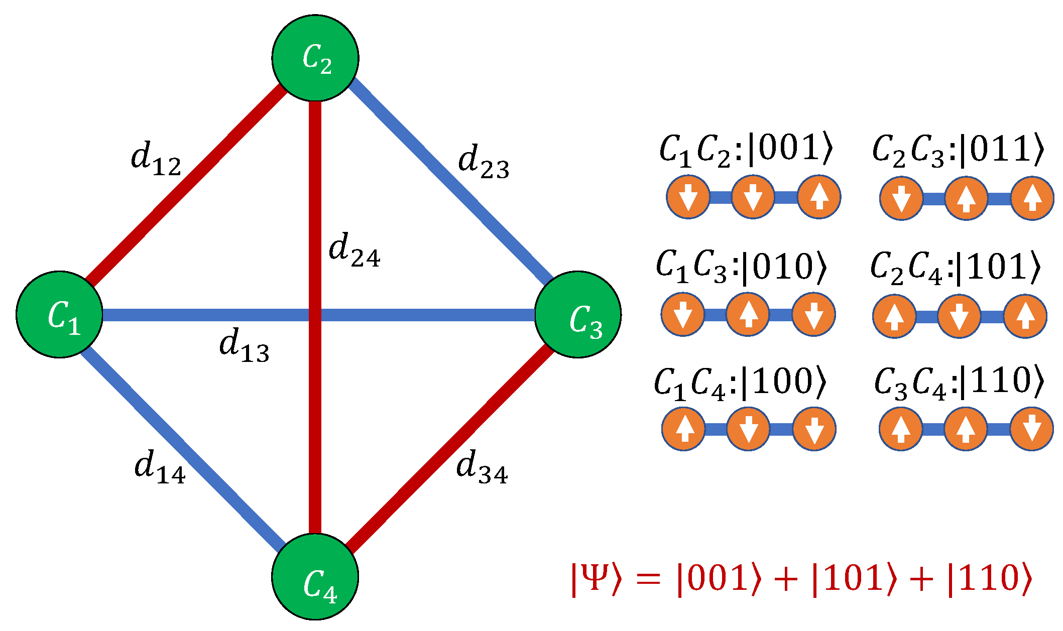
Figure 1 shows an example of our construction. We assign a quantum basis state for each path edge in the graph G. Let $e_{ij}$ be a binary index for the edge connecting cities $C_i$ and $C_j$. We encode this edge on the quantum basis state $|e_{ij}\rangle$, where the binary number describes the state of the qubits. For example $|e_{ij}\rangle =|011\rangle$ is a quantum state where the first qubit is off and the second and third qubits are on (we assume little endian ordering). For $N_E$ edges we need only $N_Q=\lceil {log}_2{N}_E\rceil$ qubits. A route on the quantum computer $|R\rangle$ is defined by a superposition of states:

$$|R\rangle ={\displaystyle \frac{1}{\sqrt{N_R}}}\sum _k|e_{\mathrm{idx}\left(R_k\right),\mathrm{idx}\left(R_{k+1}\right)}\rangle ,$$

(2)

where $N_R$ is the number of basis states in the summation. For example, the route $R=(C_3,C_2,C_5)$ is mapped to $|R\rangle ={\displaystyle \frac{1}{\sqrt{2}}}(|e_{32}\rangle +|e_{25}\rangle )$. Notice that $|R\rangle$ does not define an order for the paths $|e_{ij}\rangle$.

We define the order classically after the quantum computer is measured. Details are presented in Section 2.3.

It is straightforward to define a quantum distance operator:

$$\widehat{D}=\sum _{ij}{d}_{ij}|e_{ij}\rangle \langle e_{ij}|.$$

(3)

We can define the distance of an arbitrary quantum state $|\mathsf{\Psi }\rangle$ to be the expectation values of the quantum distance operator:

$$D_q\left(\mathsf{\Psi }\right)=\langle \mathsf{\Psi }|\widehat{D}|\mathsf{\Psi }\rangle .$$

(4)

This allows us to calculate the distance of a route R using the distance operator

$$D\left(R\right)=D_q(\mathsf{\Psi }=R).$$

(5)

However, the full cost function needs to do more than evaluate the distance of a quantum state. There must also be constraints in the cost function so that the cost is increased for quantum states that do not define true solutions of the TSP. We describe two methods for evaluating the full cost function.

2.3. Evaluating the Cost Function

The amplitude encoding offers a dense encoding of information onto the quantum register. The density of information is an advantage in that the required number of qubits is small. However, it presents a challenge when trying to evaluate the cost function. As seen in the previous section, the distance of a route can be promoted to a quantum operator. However, the cost function must also involve a constraint that only full tours should be considered as solutions. We refer to this constraint as the full-tour constraint. Typically, one would write a cost function that involves both the distance and the full tour constraint and promote this function to a quantum operator. However, it is far from obvious how one can obtain such an operator in this case. The main insight of our work is that we can evaluate the cost function without defining a corresponding quantum operator. Instead we use the probability distribution measured from the quantum computer.

In what follows, we will go into detail about how to use the measurement results of the quantum computer to determine a value for the cost function. It is important to remember that evaluating the cost function is not the same as finding a solution to the TSP. The cost function is simply a measure of how close the current state of the quantum computer is to the state that represents the solution. In order to find a solution, the quantum state must be varied. We will describe a variational quantum algorithm that can be used to find the solution in Section 2.4.

We describe two methods of evaluating the cost function given the probability distribution over the quantum basis states. Given the state of the quantum computer $|\mathsf{\Psi }\rangle$ the probability distribution is

$$w_{ij}={\left|\langle e_{ij}|\mathsf{\Psi }\rangle \right|}^2.$$

(6)

A fundamental aspect of quantum computation is that the probability distribution can be well approximated by repeated measurements of the quantum state. It is these measurement results that we use to evaluate the cost function.

2.3.1. Lagrange Multiplier Method

In this method, we evaluate the full tour constraint by extracting a route that represents a candidate for the full tour $|T\rangle$. We find the candidate tour $|T\rangle$ by consecutively evaluating the highest probability edges. The steps for finding $|T\rangle$ are as follows:

step 0

$T=\left(C_0\right)$

step 1

Find $j^{*}$ such that $w_{0j^{*}}\ge w_{0j}$ for all $j\ne 0$.

step 2

Append $C_{j^{*}}$ to the last entry in T.

step 3

Set $i^{*}=j^{*}$ and find a new $j^{*}$ such that $w_{i^{*}{j}^{*}}\ge w_{i^{*}j}$ for all j such that $C_j$ is not in T.

step 4

Append $C_{j^{*}}$ to the last entry in T.

step 5

Repeat step 3 and step 4 until all cities are reached.

To evaluate the cost function, we compare the candidate tour $|T\rangle$ to the state of the quantum computer $|\mathsf{\Psi }\rangle$

$$F\left(\mathsf{\Psi }\right)=(1-|\langle T|\mathsf{\Psi }\rangle {|}^2).$$

(7)

The full cost function is evaluated as

$$C_1(a,\mathsf{\Psi })=D_q\left(\mathsf{\Psi }\right)+aF\left(\mathsf{\Psi }\right)$$

(8)

where $D_q\left(\mathsf{\Psi }\right)$ is evaluated by taking the expectation value of the distance operator as in Equation (4) and a is a Lagrange multiplier.

There is no guarantee that the tour $|T\rangle$ found this way minimizes $F\left(\mathsf{\Psi }\right)$. However, it is guaranteed that $F\left(\mathsf{\Psi }\right)\to 0$ as $|\mathsf{\Psi }\rangle$ converges to a full tour. Therefore, minimizing $F\left(\mathsf{\Psi }\right)$ enforces the full-tour constraint.

2.3.2. Tour Averaging Method

In this method, we do not use the expectation value of the distance operator $D_q\left(\mathsf{\Psi }\right)$ in the cost function. Instead we take the average distance of a number of tours found probabilistically from the probability distribution of the quantum state.

The method for finding a tour is similar to that in the Lagrange multiplier method, except, we select each edge probabilistically. The steps to find a tour are as follows:

step 0

$T_x=\left(C_0\right)$

step 1

Select $j^{*}$ with probability $\left|\right|w_{0j^{*}}\left|\right|$.

step 2

Append $C_{j^{*}}$ to the last entry in $T_x$.

step 3

Set $i^{*}=j^{*}$ and select a new $j^{*}$ with probability $\left|\right|w_{i^{*}{j}^{*}}\left|\right|$ from any $j^{*}$ such that $C_{j^{*}}$ is not in $T_x$.

step 4

Append $C_{j^{*}}$ to the last entry in $T_x$.

step 5

Repeat step 3 and step 4 until all cities are reached.

where $\left|\right|w_{i^{*}{j}^{*}}\left|\right|=w_{i^{*}{j}^{*}}/{\sum }_j{w}_{i^{*}j}$ unless ${\sum }_j{w}_{i^{*}j}=0$ in which case $\left|\right|w_{i^{*}j}\left|\right|$ is equally distributed over all j.

We calculate the distance of the tour using Equation (1). We repeat this process to find a distribution of tours. The cost function is the average distance of all the tours

$$C_2\left(\mathsf{\Psi }\right)=\sum _x{n}_{x}D\left(T_x\right).$$

(9)

where $n_x$ is the number of times $T_x$ was found. Because every distance in the average is calculated based on a full tour, the full-tour constraint is automatically enforced.

2.3.3. Comparison of Lagrange Multiplier and Tour Averaging Methods

In the Lagrange multiplier method we interpret the quantum state as representing a single tour. We attempt to force the quantum state into an exact tour state using the Lagrange multiplier a. In the tour averaging method, we interpret the quantum state as representing a distribution of unique tours. We average over this distribution to calculate the distance. We see that while both methods use the same encoding, the interpretation of the quantum state is subtly different.

The Lagrange multiplier method gives us an extra control parameter a that may help expedite convergence. On the other hand, the evaluation of the cost function does not take full advantage of all of the information in the probability distribution as many different distributions can produce the same tour. Furthermore, there are switching points in the space of quantum states where the candidate tour changes. $F\left(\mathsf{\Psi }\right)$ is likely to be discontinuous across these switching points.

The tour averaging method does not suffer from switching points in the same way. Of course, the most probable tour will switch suddenly at certain points in the state space. However, the cost function is continuous across these points. It is unclear which method will ultimately be the most effective; however, the continuity of the cost function is a strong indication that tour averaging may be preferred.

2.4. Variational Quantum Algorithm for Solving the TSP

To demonstrate the encoding method, we perform a VQE-type algorithm. A flow chart for the algorithm is depicted in Figure 2, where the algorithm is compared to standard VQE. In both our algorithm and standard VQE, the quantum computer is used to generate a variational ansatz. The expectation value of the ansatz is then measured for a number of operators. Finally, a cost function is evaluated based on those expectation values. In standard VQE the cost function is simply a sum of expectation values. Our algorithm differs in that the cost function is a nonlinear function of expectation values. The variational parameters are then updated based on the value of the cost function using a classical optimization routine.

For the demonstration, we use the hardware-efficient ansatz [30] as the variational ansatz and we use Simultaneous Perturbations Stochastic Approximation (SPSA) as the classical optimization routine. During each iteration of the optimization routine, we evaluate the cost function based on one of the two methods described in Section 2.3.

Two layers of the hardware-efficient ansatz are shown in Figure 3. Each layer consist of a stack of Y-rotations followed by alternating CNOT gates. The Y-rotations are parameterized by the variational parameter ${\varphi }_{ql}$ where q indicates the qubit and l indicates the layer. Throughout our demonstration, we use a 2-layer ansatz.

2.5. Algorithm Complexity

The advantage of our encoding is that it requires a small number of qubits. To make that statement precise, let us analyze the method. Our method maps each path between pairs of cities onto a basis state. If there are $N_C$ cities, then there are $N_C^2$ ordered city pairs. Pairing a city with itself does not define an edge, thus, there are at most $N_E=N_C^2-N_C$ directed edges between city pairs. If we restrict the problem so that the return path has the same distance as the forward path then we only need to consider half of the total number of edges.

Given a number of qubits $N_Q$, the number of basis states is $N_B=2^{N_Q}$. We need a basis state for each edge. Therefore, we need a number of qubits equal to

$$N_Q=\lceil {log}_2(N_C^2-N_C)\rceil .$$

(10)

Another factor that contributes to the algorithm complexity is the required number of ansatz layers, known as the circuit depth. The depth of the quantum circuit required to optimize the route is an open problem. However, it has been demonstrated that VQE can solve complex problems with reasonably shallow circuits [30].

Another factor in the complexity of the algorithm is the number of shots required to achieve an accurate estimate of the cost function. The standard method of calculating expectation values of an operator on a quantum computer is to separate the operator into a sum of Pauli strings. Each set of commuting Pauli strings must be measured in a separate basis. As the distance operator $\widehat{D}$ can be constructed from Pauli-Z and identity operators, it requires only a single basis to be measured. Similarly, while we have to calculate $\mathcal{O}\left(N_C^2\right)$ different $w_{ij}$, they all can be calculated from the same measurement basis. Thus, the number of shots $N_S$ required to get an expectation value to an accuracy of $ϵ$ scales as [37,38]

$$N_S=\mathcal{O}\left(1/{ϵ}^2\right).$$

(11)

Finally, evaluating the cost function from the results of the quantum computer is achieved by a classical algorithm that scales as

$$N_V\le \sum _{i=1}^{N_C}\sum _{j=1}^{i}1<N_C^2.$$

(12)

Thus, assuming we do not need exponentially many ansatz layers, no part of the algorithm scales exponentially with the number of cities.

2.6. Comparison to Basis Encoding

The main advantage of our method is the use of amplitude encoding to reduce the required number of qubits. In the standard basis encoding [17,35], one must have a unique basis state for each possible route. In general, there are $N_p=(N_C-1)!$ unique routes. As stated previously, the number of basis states in the quantum computer is $N_B=2^{N_Q}$. Therefore, one needs at least $N_Q^{\mathrm{basis}}=\lceil {log}_2([N_C-1]!)\rceil$ qubits for a basis encoding. Often, the encoding is simplified if you associate each qubit with an edge so that $N_Q^{\prime \mathrm{basis}}=N_C^2-N_C$. In either case, both $N_Q^{\mathrm{basis}}$ and $N_Q^{{\prime }^{\mathrm{basis}}}$ are exponentially larger than the number of qubits required for the amplitude encoding $N_Q$. This improvement in qubit resources is due to the fact that, in the basis encoding, much of the quantum information that can be registered on a quantum computer is not used. In particular, in a basis encoding, different linear combinations of basis states do not carry unique information about the problem. The advantage of basis encoding is that the information about the problem is simple to read off of the quantum computer. For example, one may consider only the most probable basis state in the measured probability distribution to be relevant. This greatly simplifies the evaluation of the cost function. However, as we show, various strategies exist for evaluating costs functions for an amplitude encoding.

One open question is how the convergence of the variational method will compare between the basis and amplitude encodings. This question is beyond the scope of the current work. The small graphs that we consider will not be able to resolve the question of convergence as both encodings should converge quickly for small graphs. The real question is how the convergence will change as we increase the size of the graphs. For large graphs, the hardware-efficient ansatz is not likely to be useful for either encoding. A systematic exploration of various ansatzes is required to make any definite claims about scalability.

2.7. Quantum Advantage

Another open question is whether it is possible to obtain a quantum advantage using the our method. Because of the logarithmic scaling in the number of qubits, classical simulations of the quantum computing portion of the algorithm will be viable for even relatively large problems. However, there are still exponentially more basis states than the number of qubits and so the classical simulation still requires exponentially more resources than when using a quantum computer.

However, there are many other classical algorithms that can be used to address the TSP. A full comparison of each method to our own is beyond the scope of this work, but we will try to provide some insights. Firstly, our algorithm is certainly efficient in the number of qubits. In addition, the evaluation of the cost function scales with the number of measurement shots taken from the quantum computer. Thus, the question becomes, how many quantum operations are required in order to generate a probability distribution in which a good approximation of the cost function can be calculated using a small number of shots.

The number of required quantum operations is an open question for variational algorithms in general. The number of quantum operations depends on the ansatz that is used. For certain ansatzes, arguments have been made that a quantum advantage can be obtained for certain problems once we have fully error-corrected quantum computers [29]. However, other ansatzes are specifically designed for near-term quantum computers and they may not scale in the long term [30]. We have demonstrated our method with the hardware efficient ansatz. What other ansatzes are applicable is still an open question.

3. Demonstration of the Algorithm

We perform all of our calculations on error-free classical simulations of the quantum computer. The simulator is built in python and uses matrix multiplication to represent the action of quantum logic gates. The calculations demonstrate how the algorithm will function under ideal conditions, without quantum decoherence or readout errors.

We do not expect the effect of quantum errors to be worse for our method than for any other. The magnitude of the quantum errors will depend on the ansatz. For the hardware efficient that we use, quantum errors have been shown to be minimal [30].

3.1. Considerations for the Lagrange Multiplier a

The value of a in Equation (8) determines how strictly the algorithm demands that the quantum state represents a full tour. We treat a as a free parameter that can vary during optimization. In this way a acts as a Lagrange multiplier. Critically, cost functions should not be minimized when they involve Largrange multipliers. Instead, we search for a saddle point in the parameter space where the cost function is maximized with respect to a but minimized with respect to the other parameters. Because $F\left(\theta \right)$ is a positive-definite function, we know that a should monotonically increase during optimization. Therefore, we can choose, a priori, to increase a at a given rate during optimization.

Figure 4 shows the cost functions during each iteration k of the algorithm, where the parameter $a=k/500$ increases with the iterations. The cost function is separated into the distance portion $D_q\left(\mathsf{\Psi }\right)$ and the tour restriction portion $F\left(\mathsf{\Psi }\right)$. We find that the distance portion of the cost function is originally optimized past the point of a full tour. As a increases, the route restriction portion of the cost function begins to dominate the optimization and the quantum state is pushed into a full tour. The green vertical lines in Figure 4 divide the iterations into regions with different candidate tours. The candidate tour in a given iteration region is indicated on the figure by the route R, where the arrows point to the regions in which R is applicable. We see that $D_q\left(\mathsf{\Psi }\right)$ is smooth across these boundaries but $F\left(\mathsf{\Psi }\right)$ can be discontinuous. Despite these discontinuities, we find the optimal route within 100 iterations. Even after the optimal tour is found, the cost function continues to fluctuate until it converges around 1000 iterations.

3.2. Dealing with Non-Edge States

In general, there are basis states that do not correspond to any edge. If these states are in the linear combination that defines the quantum state, then they contribute to the cost function through $F\left(\mathsf{\Psi }\right)$. Additionally, one may decide to assign large distances to these non-edge basis states so that they also contribute to $D_q\left(\mathsf{\Psi }\right)$; however, adding distances to the non-edge basis states tends to make convergence worse. Figure 5 shows the cost function during the iterations of the algorithm. The cost function is separated into the distance portion $D_q\left(\mathsf{\Psi }\right)$ and the route restriction portion $F\left(\mathsf{\Psi }\right)$. In Figure 5, we assign a weight of $d_{\mathrm{off}}=0$ to basis states that do not represent an edge. In this case the optimal route is found within 70 iterations. In Figure 5b, we assign a weight of $d_{\mathrm{off}}=4$ to these states. In this case the optimal route is not found until over 90 iterations. We see that the algorithm takes longer to find the shortest distance route when $d_{\mathrm{off}}=4$. It appears that these non-edge states act as a catalyst to improve optimization times for the algorithm.

3.3. Parameter Searches

To study the effectiveness of our scheme we perform a search of its hyperparameters. The hyperparameters define the SPSA optimization scheme. Specifically, we investigated the effect of varying the perturbation size and the learning rate. We call $d\varphi$ the perturbation size and g the learning rate and they play the following role in the SPSA algorithm. At each iteration of the optimization procedure, the SPSA algorithm compares the current value of the cost function to the value of a nearby state where every parameter in the ansatz is adjusted by an amount $d{\overline{\varphi }}_{ql}=\pm d\varphi$ where ± is chosen randomly for every q and l. Based on the difference in the value of the cost function $dC$, the parameters for the next iteration are changed by an amount $d{\varphi }_{ql}=-g\times dC\times d{\overline{\varphi }}_{ql}$.

3.3.1. The Uniform Distribution

For a test case we consider the random selected graph shown in Figure 6. We create this graph from random symmetric $N\times N$ matrices. The matrix elements are generated from the uniform distribution between 0 and 1. The matrices are then symmetrized. The Python package NetworkX 3.5 is used to translate these random matrices into graphs. This randomly selected graph has the shortest route of length 1.66, following the path shown in red. This shortest route is found using brute force by looping over all routes and finding the one with the shortest length. The quantum algorithm described above is applied to this graph.

We define $D_{\mathrm{exact}}$ as the distance of the shortest route as computed by brute force methods. We define $\Delta D$ as the difference between the results of our algorithm and $D_{\mathrm{exact}}$. We will analyze the relative error $\Delta D/D_{\mathrm{exact}}$. In Figure 7, we plot the relative error after 400 iterations as a function of the hyperparameters. We performed this parameter search for several random seeds. As with many optimization routines there are optimal choices of parameters. Perturbation sizes and learning rates that are too small increase the convergence time; however, if these hyperparameters are too large, we may overshoot the target state. Overall, the convergence of the algorithm is acceptable over a broad range of parameters as shown by this search. We define the basin of convergence as the region in parameter space where the relative error is minimized. If this basin is smooth then fine tuning the hyperparameters is not necessary. In Figure 7, one finds a basin of convergence centered around a perturbation size $d\varphi \approx 0.4$ and a learning rate $g\approx 0.3$. The basin is nearly flat; however, the basin boundaries are sharp. The discontinuity in the relative error could make parameter searches difficult as we scale up the problem. As we will see, these discontinuities are removed for certain distributions and for the tour averaging method.

3.3.2. Alternative Distributions

Above, we generate the graphs by selecting matrix elements from the uniform distribution. This is far from the only option. The distribution used to generate the graph can have major consequences on the convergence of the algorithm.

We repeat the analysis for distances drawn from the normal Figure 8a, exponential Figure 8b, and gamma distributions Figure 8c. This is performed by drawing elements of our distance matrix, $d_{ij}$, from the specified distribution. Because the distance matrix is symmetric, we only need to compute elements above the diagonal where $j>i$. Elements below the diagonal are obtained through symmetry: $d_{ij}=d_{ji}$, and elements on the diagonal are zero. In the case of the normal distribution, draws that are negative are rejected. We find convergence for a broad range of hyperparameters for the normal and exponential distributions. For the normal distribution we find a basin of convergence centered around $d\varphi \approx 0.15$ and $g\approx 0.2$. For the exponential distribution the basin is shifted slightly in perturbation size, being centered closer to $d\varphi \approx 0.2$. In both cases, the basin is noisy, having sporadic points of non-convergence within the basin. Also, in both cases there is a relatively flat shelf for low learning rates $g\lesssim 0.1$ that extends across the perturbation size. Furthermore, the basin, in both cases, does not have sharp edges. The smoothness of the basin can help with finding optimal hyperparameters. However, the sporadic nature of the basin indicates that careful tuning of the hyperparameters may be necessary for these distributions.

Throughout the entire hyperparameter scan, the relative error was never larger than 0.25 for the gamma distribution. Furthermore we find that in the range centered around a perturbation size $d\varphi \approx 0.08$ with a learning rate $g\lesssim 0.25$, the relative error tends to be better. However, this basin is noisy. Thus, it may be necessary to fine-tune the hyperparameters in order to find good convergence.

3.3.3. Tour Averaging Method

As a test of the tour averaging procedure, we apply it to the same graph as shown in Figure 6 with distances taken from the normal distribution. Figure 9 shows the evolution of the cost function. We see that the cost function converges towards the optimal solution without discontinuous jumps due to tour switching. The small discontinuities in the data are due to the discontinuous parameter perturbations used in the SPSA optimizer.

We also perform a hyperparameter search for this alternative cost function, shown in Figure 10. Again, perturbation size and learning rate are varied and the deviation between the final value of the cost function and the optimal value is plotted. As in the Lagrange multiplier method, we find a broad basin of convergence for $d\varphi \lesssim 0.4$ and $g\lesssim 0.2$. Unlike in the Largrange multiplier method, the boundaries of the basin are smooth. The smoothness of the basin boundaries is a positive feature of the tour averaging method. It means that we can find the basin following the gradient of the cost function in the hyperparameter space. Additionally, the relative error is flat across the basin meaning that no fine tuning of the hyperparameters is necessary.

4. Conclusions

Our method has provided an exponential reduction in the number of qubits required to encode and solve the TSP on a quantum computer. We have demonstrated the efficacy of our method by simulating the quantum algorithm applied to four- and five-node graphs. The heart of our method is an amplitude encoding which is applicable to many different types of quantum algorithms. We have demonstrated that the encoding works particularly well for variational quantum algorithms. We have demonstrated the robustness of the encoding by considering two different evaluation methods for the cost function.

The robustness of our procedure is assessed by testing for many randomized graphs with different hyperparameters used for the variational part of the algorithm. We have found broad regions in the space of hyperparameters where exact convergence to the shortest route is found for most probability distributions. The work presented herein indicates that at least certain TSP graphs are efficiently solvable using amplitude encodings on a quantum computer.

References

1. Lawler, E.L.; Wood, D.E. Branch-and-Bound Methods: A Survey. Oper. Res. 1966, 14, 699–719. [Google Scholar] [CrossRef]
2. Padberg, M.; Rinaldi, G. Optimization of a 532-city symmetric traveling salesman problem by branch and cut. Oper. Res. Let. 1987, 6, 1–7. [Google Scholar] [CrossRef]
3. Little, J.D.C.; Murty, K.G.; Sweeney, D.W.; Karel, C. An Algorithm for the Traveling Salesman Problem. Oper. Res. 1963, 11, 972–989. [Google Scholar] [CrossRef]
4. Held, M.; Karp, R.M. The traveling-salesman problem and minimum spanning trees: Part II. Math. Program. 1971, 1, 6–25. [Google Scholar] [CrossRef]
5. Lin, S.; Kernighan, B.W. An Effective Heuristic Algorithm for the Traveling-Salesman Problem. Oper. Res. 1973, 21, 498–516. [Google Scholar] [CrossRef]
6. Geem, Z.W.; Kim, J.H.; Loganathan, G.V. A New Heuristic Optimization Algorithm: Harmony Search. Simulation 2001, 76, 60–68. [Google Scholar] [CrossRef]
7. Laporte, G.; Martello, S. The selective travelling salesman problem. Discret. Appl. Math. 1990, 26, 192–207. [Google Scholar] [CrossRef]
8. Karg, R.L.; Thompson, G.L. A Heuristic Approach to Solving Travelling Salesman Problems. Manag. Sci. 1964, 10, 225–248. [Google Scholar] [CrossRef]
9. Bhide, S.; John, N.; Kabuka, M.R. A real-time solution for the traveling salesman problem using a Boolean neural network. In Proceedings of the EEE International Conference on Neural Networks, San Francisco, CA, USA, 28 March 1993. [Google Scholar]
10. Golden, B.; Naji-Azimi, Z.; Raghavan, S.; Salari, M.; Toth, P. The Generalized Covering Salesman Problem. INFORMS J. Comput. 2012, 24, 534–553. [Google Scholar] [CrossRef]
11. Rana, S.; Srivastava, S. Solving Travelling Salesman Problem Using Improved Genetic Algorithm. Ind. J. Sci. Technol. 2017, 10, 1–6. [Google Scholar] [CrossRef]
12. Grover, L.K. A Fast Quantum Mechanical Algorithm for Database Search. In Proceedings of the Twenty-Eighth Annual ACM Symposium on Theory of Computing, Philadelphia, PA, USA, 22 May 1996. [Google Scholar]
13. Goswami, D.; Karnick, H.; Jain, P.; Maji, H.K. Towards Efficiently Solving Quantum Traveling Salesman Problem. arXiv 2004, arXiv:0411013. [Google Scholar] [CrossRef]
14. Bang, J.; Ryu, J.; Lee, C.; Yoo, S.; Lim, J.; Lee, J. A quantum heuristic algorithm for the traveling salesman problem. J. Korean Phys. Soc. 2012, 61, 1944–1949. [Google Scholar] [CrossRef]
15. Moylett, D.J.; Linden, N.; Montanaro, A. Quantum speedup of the traveling-salesman problem for bounded-degree graphs. Phys. Rev. A 2017, 95, 3. [Google Scholar] [CrossRef]
16. Kitaev, A.Y. Quantum measurements and the Abelian Stabilizer Problem. arXiv 1995, arXiv:9511026. [Google Scholar] [CrossRef]
17. Srinivasan, K.; Satyajit, S.; Behera, B.K.; Panigrahi, P.K. Efficient quantum algorithm for solving travelling salesman problem: An IBM quantum experience. arXiv 2018, arXiv:1805.10928. [Google Scholar] [CrossRef]
18. van Dam, W.; Mosca, M.; Vazirani, U. How powerful is adiabatic quantum computation? In Proceedings of the 42nd IEEE Symposium on Foundations of Computer Science, Washington, DC, USA, 14 October 2001. [Google Scholar]
19. Smelyanskiy, V.N.; Toussaint, U.V.; Timucin, D.A. Simulations of the adiabatic quantum optimization for the Set Partition Problem. arXiv 2001, arXiv:0112143. [Google Scholar]
20. Reichardt, B.W. The Quantum Adiabatic Optimization Algorithm and Local Minima. In Proceedings of the Thirty-Sixth Annual ACM Symposium on Theory of Computing, Chicago, IL, USA, 13 June 2004. [Google Scholar]
21. Farhi, E.; Goldstone, J.; Gutmann, S.; Lapan, J.; Lundgren, A.; Preda, D. A Quantum Adiabatic Evolution Algorithm Applied to Random Instances of an NP-Complete Problem. Science 2001, 292, 472–475. [Google Scholar] [CrossRef]
22. Kieu, T.D. The travelling salesman problem and adiabatic quantum computation: An algorithm. Quantum Inf. Process. 2019, 18, 3. [Google Scholar] [CrossRef]
23. Apolloni, B.; Carvalho, C.; de Falco, D. Quantum stochastic optimization. Stoch. Proc. Appl. 1989, 33, 233–244. [Google Scholar] [CrossRef]
24. Kadowaki, T.; Nishimori, H. Quantum annealing in the transverse Ising model. Phys. Rev. E 1998, 58, 5355–5363. [Google Scholar] [CrossRef]
25. Irie, H.; Wongpaisarnsin, G.; Terabe, M.; Miki, A.; Taguchi, S. Quantum Annealing of Vehicle Routing Problem with Time, State and Capacity. EPJ Quantum Technol. 2019, 145–156. [Google Scholar]
26. Crispin, A.; Syrichas, A. Quantum Annealing Algorithm for Vehicle Scheduling. In Proceedings of the 2013 IEEE International Conference on Systems, Man, and Cybernetics, Washington, DC, USA, 13 October 2013. [Google Scholar]
27. Sao, M.; Watanabe, H.; Musha, Y.; Utsunomiya, A. Application of digital annealer for faster combinatorial optimization. Fujitsu Sci. Tech. J. 2019, 55, 45–51. [Google Scholar]
28. Salehi, Ö.; Glos, A.; Miszczak, J.A. Unconstrained binary models of the travelling salesman problem variants for quantum optimization. Quantum Inf. Process. 2022, 21, 67. [Google Scholar] [CrossRef]
29. Peruzzo, A.; McClean, J.; Shadbolt, P.; Yung, M.-H.; Zhou, X.-Q.; Love, P.J.; Aspuru-Guzik, A.; O’Brien, J.L. A variational eigenvalue solver on a photonic quantum processor. Nat. Commun. 2014, 5, 1. [Google Scholar] [CrossRef] [PubMed]
30. Kandala, A.; Mezzacapo, A.; Temme, K.; Takita, M.; Brink, M.; Chow, J.M.; Gambetta, J.M. Hardware-efficient variational quantum eigensolver for small molecules and quantum magnets. Nature 2017, 549, 242–246. [Google Scholar] [CrossRef]
31. McClean, J.R.; Romero, J.; Babbush, R.; Aspuru-Guzik, A. The theory of variational hybrid quantum-classical algorithms. New J. Phys. 2016, 18, 023023. [Google Scholar] [CrossRef]
32. O’Malley, P.J.J.; Babbush, R.; Kivlichan, I.D.; Romero, J.; McClean, J.R.; Barends, R.; Kelly, J.; Roushan, P.; Tranter, A.; Ding, N.; et al. Scalable Quantum Simulation of Molecular Energies. Phys. Rev. X 2016, 13, 031007. [Google Scholar] [CrossRef]
33. Farhi, E.; Goldstone, J.; Gutmann, S. A Quantum Approximate Optimization Algorithm. arXiv 2014, arXiv:1411.4028. [Google Scholar] [CrossRef]
34. Mohanty, N.; Behera, B.K.; Ferrie, C. Analysis of The Vehicle Routing Problem Sovled via Hybrid Quantum Algorithms in Presence of Noisy Channels. IEEE Trans. Quantum Eng. 2023, 4, 3101514. [Google Scholar] [CrossRef]
35. Azad, U.; Behera, B.K.; Ahmed, E.A.; Panigrahi, P.K.; Farouk, A. Solving Vehicle Routing Problem Using Quantum Approximate Optimization Algorithm. IEEE Trans. Intel. Transp. Syst. 2022, 24, 7564–7573. [Google Scholar] [CrossRef]
36. Gonzalez-Conde, J.; Watts, T.W.; Rodriguez-Grasa, P.; Sanz, M. Efficient quantum amplitude encoding of polynomial functions. Quantum 2024, 8, 1297. [Google Scholar] [CrossRef]
37. Rubin, N.C.; Babbush, R.; McClean, J. Application of fermionic marginal constraints to hybrid quantum algorithms. New J. Phys. 2018, 20, 5. [Google Scholar] [CrossRef]
38. Wecker, D.; Hastings, M.B.; Troyer, M. Progress towards practical quantum variational algorithms. Phys. Rev. A 2015, 92, 10. [Google Scholar] [CrossRef]
Figure 1. A simple graph connecting four cities. The cities are depicted by green circles labeled C 1 , C 2 , C 3 , and C 4 . Each city is connected to all other cities as depicted by the blue and red lines. The distance between cities C i and C j is labeled d i j , which need not be proportional to the length of the line. We encode this graph onto qubits as shown on the right. Each qubit is depicted as an orange circle with an arrow representing the state of the qubit. Each pair of cities is encoded onto a basis state of the quantum computer. The route R = ( C 1 , C 2 , C 4 , C 3 ) is shown in red. This route corresponds to the quantum state | Ψ = ( | 001 + | 101 + | 110 ) / 3 as shown in the bottom right corner.
Quantumrep 07 00032 g001
Figure 2. Flow diagram for standard VQE (top) and our algorithm (bottom). Here, ϕ is a set of variational parameters, O ^ i are arbitrary operators, o i ( Ψ ) are expectation values, and f is an arbitrary function.
Quantumrep 07 00032 g002
Figure 3. Two layers of the hardware-efficient ansatz for four qubits. Each horizontal line represents a qubit. Each box represents a parameterized Y-rotation gate. The vertical lines connected to circles represent controlled not gates, where the filled circle is attached to the control qubit and the open circle, inscribed with an “X”, is attached to the target qubit.
Quantumrep 07 00032 g003
Figure 4. Plot of the costs as a function of optimization iteration for a four city graph. The path between each city is set to d i j = 1 except for d a c = d c d = 0.5 and d b d = 0.1 . The Lagrange multiplier changes during optimization. At iteration k of the optimization procedure, a = k / 500 . The thin orange line is the overlap cost F ( Ψ ) and the thick blue line is the distance cost D q ( Ψ ) . The vertical green lines show the points where the candidate tour changes.
Quantumrep 07 00032 g004
Figure 5. Plot of the costs as a function of time for a four city graph. The path between each city is set to d i j = 1 except for d a c = d c d = 0.5 and d b d = 0.1 . States which do not encode paths are artificially given a distance of (a) d off = 0 and (b) d off = 4 . At iteration k of the optimization procedure, a = k / 500 . The thin orange line is the overlap cost F ( Ψ ) and the thick blue line is the distance cost D q ( Ψ ) . The vertical green lines show the points where the candidate tour changes.
Quantumrep 07 00032 g005
Figure 6. Randomized city locations with the shortest route for visiting all of them shown in red and unused connections shown in blue. This route starts at city “ C 1 ” and ends at city “ C 3 ”. This shortest route has a length of 1.66. Distances for this map are drawn from the set 0 , 1 with a uniform probability distribution. Values of distances between cities are printed at midpoints.
Quantumrep 07 00032 g006
Figure 7. Relative error Δ D / D exact as a function of the optimization hyperparameters, learning rate g, and perturbation size d ϕ . The distances for the graph are taken from the uniform distribution.
Quantumrep 07 00032 g007
Figure 8. Relative error Δ D / D exact as a function of the optimization hyperparameters, lerning rate g and perturbation size d ϕ . The distances of the graph are taken from (a) the normal distribution, (b) the exponential distribution, and (c) the gamma distrition.
Quantumrep 07 00032 g008
Figure 9. Alternative cost function evolution for our variational circuit training on the graph at Figure 6. The grey lines represent all possible route lengths and we note convergence to the smallest length in about 400 steps. At each iteration of this plot, 300 sample routes are chosen to compute an average.
Quantumrep 07 00032 g009
Figure 10. Relative error Δ D / D exact as a function of the optimization hyperparameters, learning rate g, and perturbation size d ϕ . The error is found using the tour averaging method. The distances of the graph are taken form the uniform distribution.
Quantumrep 07 00032 g010
Disclaimer/Publisher’s Note: The statements, opinions and data contained in all publications are solely those of the individual author(s) and contributor(s) and not of MDPI and/or the editor(s). MDPI and/or the editor(s) disclaim responsibility for any injury to people or property resulting from any ideas, methods, instructions or products referred to in the content.