Superoperator Approach to the Lindbladian Dynamics of a Mirror-Field System

Abstract

We use superoperator techniques to solve the master equation for the interaction between a single-mode quantized field and a single mechanical mode of a moving mirror, which is coupled to a zero-temperature reservoir that damps its amplitude. The solution we provide allows for its application in any initial state of the combined system. Furthermore, we obtain solutions to the stationary master equation for an initial number state for the field that is consistent with the result obtained for the average number of phonons.

1. Introduction

A cavity optomechanical system consists of an optical or microwave cavity with a movable mechanical component that can sustain collective vibrational modes [1,2,3,4,5]. These systems have attracted significant attention due to their potential applications in both fundamental physics and quantum technologies [6]. Some examples include cooling of mechanical motion to its quantum ground state [7,8], the generation of nonclassical states of light [9], and displacement sensing with precision beyond the standard quantum limit [10].

A basic example of such a system is a cavity with two mirrors: one fixed and the other movable, which is coupled to a spring, allowing for harmonic oscillations influenced by the radiation pressure of the field inside the cavity. This configuration enables a parametric modulation of the optical mode frequency of the cavity through the motion of the mirror. Generalizations of it have been proposed that include the interaction with a two-level atom [11].

As the system cannot be completely isolated, there exists a coupling with its environment, introducing decoherence and dissipation effects such as photon leakage from the cavity and damping of the mechanical oscillator’s motion. On the one hand, Mancini et al. [12] studied the case where the radiation mode lost energy much faster than the mechanical oscillator. By following an operator perturbation procedure, they managed to solve the system’s master equation. On the other hand, Bose and collaborators [13] solved the master equation for the optomechanical system considering the effect of damping on the mechanical oscillator’s amplitude by employing a technique that alternated between applying unitary and non-unitary evolution of the master equation over small time intervals, later taking the limit as time approached zero. In [14], operator techniques were employed to transform the master equation of the optomechanical system, when subjected to environmental effects, into a master equation amenable to an analytical solution. In particular, they found that the optomechanical system with damping behaved as a free mechanical harmonic oscillator coupled to an environment, provided that the initial state of the cavity field was a thermal state.

The approach of superoperators for solving the master equation of a system has received little attention. The superoperator techniques involved in this approach consist, for instance, of defining superoperators that form a closed algebra under the commutation operation, allowing for direct integration of the master equation and enabling the proposal of an ansatz to factorize the exponential of superoperators [15,16]. Alternatively, these superoperators can be used to apply transformations to the system’s density operator to rewrite the master equation into a form where its terms can be more easily manipulated, thus facilitating its analytical solution.

In this work, we employ superoperator techniques to solve the master equation in its Lindblad form for an optomechanical system subject to damping in the amplitude of the mechanical oscillator. Additionally, we compute and analyze the behavior of the average number of photons and, in particular, phonons in the damped optomechanical system, under the assumption that both the electromagnetic field and the mechanical oscillator are initially in coherent states. We also provide a steady state solution for the master equation when the initial field state is given by a Fock state.

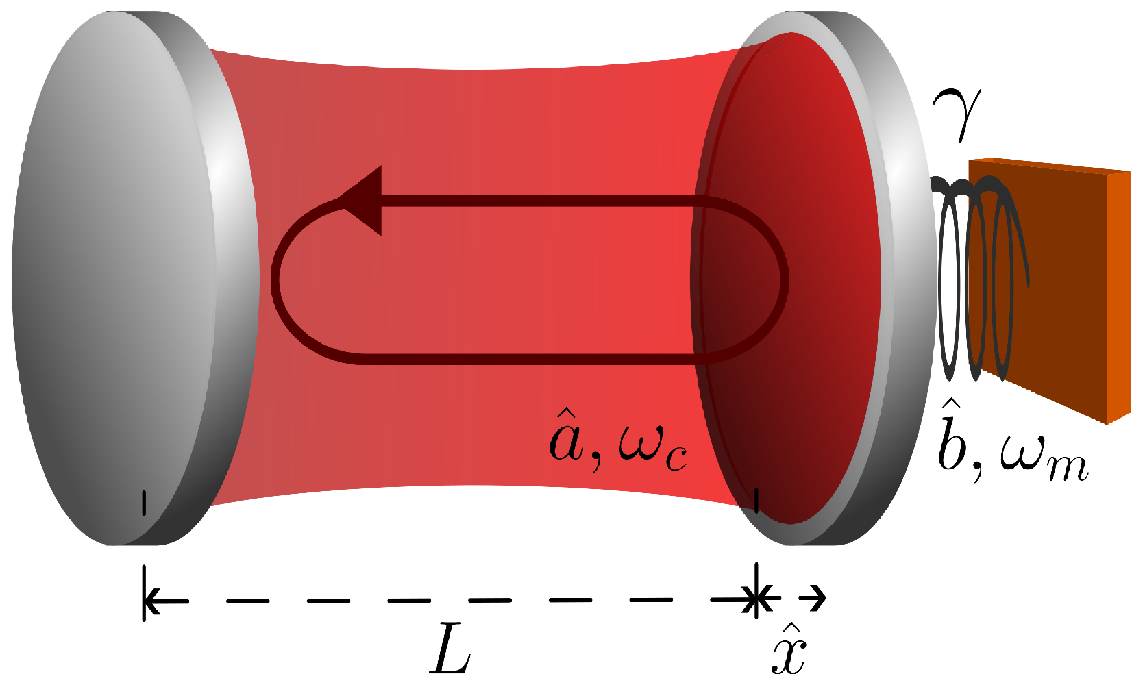
2. The Basic Optomechanical System

The system under consideration is a Fabry–Pérot cavity with one fixed end mirror and the other attached to a spring, allowing it to oscillate due to the radiation pressure force exerted by the cavity field, as shown in Figure 1. The Hamiltonian that describes this system, for a single-mode quantized field and a single mechanical mode of a moving mirror, without damping, is given by [17] (we set $\hslash =1$)

$$\widehat{H}=\omega \left(\widehat{x}\right)\left(\widehat{n}+{\displaystyle \frac{1}{2}}\right)+\left({\displaystyle \frac{{\widehat{p}}^2}{2m}}+{\displaystyle \frac{m{\omega }_m^2}{2}}{\widehat{x}}^2\right),$$

(1)

where $\widehat{n}={\widehat{a}}^{†}\widehat{a}$ is the number operator of the cavity field, $\widehat{x}$ and $\widehat{p}$ are the position and momentum operators of the mechanical oscillator, with m and ${\omega }_m$ being its mass and natural frequency, respectively. The function $\omega \left(\widehat{x}\right)$ represents the angular frequency of the cavity mode, given by [2,3]

$$\omega \left(\widehat{x}\right)={\displaystyle \frac{{\omega }_c}{1+\frac{\widehat{x}}{L}}}\approx {\omega }_c\left(1-{\displaystyle \frac{\widehat{x}}{L}}\right),$$

(2)

where L and ${\omega }_c$ represent the length and the angular frequency of the cavity in the absence of interaction, respectively. We assume that the mirror displacement is small compared with the cavity length, i.e., $L\gg x$. This setup enables the parametric modulation of the optical mode frequency of the cavity through the motion of the mirror, that is, we have a dispersive [18] coupling between optical and mechanical degrees of freedom. As quantum harmonic oscillators are naturally described in terms of ladder operators, we use the relations $\widehat{x}=\sqrt{{\displaystyle \frac{1}{2m{\omega }_m}}}({\widehat{b}}^{†}+\widehat{b})$ and $\widehat{p}=i\sqrt{{\displaystyle \frac{m{\omega }_m}{2}}}\left({\widehat{b}}^{†}-\widehat{b}\right)$, where $\widehat{b}$ is the annhilation operator of the mechanical mode, to rewrite Equation (1) as

$$\widehat{H}={\omega }_c\widehat{n}+{\omega }_m\widehat{N}-G_0({\widehat{b}}^{†}+\widehat{b})\left(\widehat{n}+{\displaystyle \frac{1}{2}}\right)+{\displaystyle \frac{{\omega }_c+{\omega }_m}{2}},$$

(3)

where $G_0={\displaystyle \frac{{\omega }_c}{L}}\sqrt{{\displaystyle \frac{1}{2m{\omega }_m}}}$ is identified as the optomechanical coupling constant.

Figure 1. Diagram of an optomechanical cavity system. A Fabry–Pérot cavity with equilibrium length L contains an optical mode with frequency ${\omega }_c$ and the annihilation operator for the electromagnetic mode is $\widehat{a}$. One of the cavity mirrors is mounted on a mechanical oscillator with frequency ${\omega }_m$ and the annihilation operator for the mechanical mode is $\widehat{b}$. The optomechanical interaction arises due to the radiation pressure exerted by the optical field on the movable mirror, where $\widehat{x}$ represents the displacement of the mechanical oscillator. The mechanical dissipation is characterized by the damping rate $\gamma$.

3. Optomechanical System with Damping in the Mechanical Oscillator

We consider an optomechanical system in which the movable mirror, modeled as a harmonic oscillator, is coupled to a zero-temperature environment, which damps the amplitude of the mechanical oscillator. Elsewhere, we will study the case of a thermal bath at a finite temperature. This is justified by assuming that we are considering a high-quality-factor cavity, meaning mirrors with a high reflectivity, which allows the mirror damping rate to be several orders of magnitude greater than the damping rate due to light leakage from the cavity. The master equation describing the dynamics of the damped optomechanical system is given by (we set $\hslash =1$)

$${\displaystyle \frac{d\widehat{\rho }}{dt}}=-i\left[\widehat{H},\widehat{\rho }\right]+\gamma \mathcal{L}\left[\widehat{b}\right]\widehat{\rho },$$

(4)

where $\widehat{\rho }$ is the density operator of the entire system and $\widehat{H}$ is the Hamiltonian from Equation (3). The term $\mathcal{L}\left[\widehat{b}\right]\widehat{\rho }=2\widehat{b}\widehat{\rho }{\widehat{b}}^{†}-({\widehat{b}}^{†}\widehat{b}\widehat{\rho }+\widehat{\rho }{\widehat{b}}^{†}\widehat{b})$ is the Lindblad superoperator and $\gamma$ is the damping constant of the mechanical oscillator.

Some authors [12,13,19] generally describe the dynamics of the optomechanical system by assuming that the Hamiltonian of the system is

$$\widehat{H}={\omega }_c\widehat{n}+{\omega }_m\widehat{N}-G_0\widehat{n}(\widehat{b}+{\widehat{b}}^{†}),$$

(5)

that is, they neglect the contribution $G_0({\widehat{b}}^{†}+\widehat{b})/2$ in the Hamiltonian (3). This approximation is valid as long as the number of photons is much greater than $1/2$. However, as we will show, it is possible to perform a transformation to eliminate the linear term in the position of the mechanical oscillator in Equation (3), thereby obtaining the standard expression of the Hamiltonian.

3.1. Obtaining the Standard Hamiltonian in the Optomechanical Master Equation

As mentioned earlier, the Hamiltonian commonly used to describe the optomechanical system is the one given in Equation (5); however, we can recover that standard form of the Hamiltonian starting from the master equation in Equation (4), whose Hamiltonian is given by Equation (3), by performing the following transformation:

$$\widehat{\rho }={\widehat{D}}_b\left(\alpha \right)\widehat{\tilde{\rho }}{\widehat{D}}_b^{†}\left(\alpha \right),$$

(6)

where ${\widehat{D}}_{\widehat{b}}\left(\alpha \right)=exp[\alpha {\widehat{b}}^{†}-{\alpha }^{*}\widehat{b}]$ is the Glauber displacement operator [20]. Then, if $\alpha ={\displaystyle \frac{G_0}{2}}{\displaystyle \frac{{\omega }_m+i\gamma }{{\gamma }^2+{\omega }_m^2}}$, the master equation is transformed into

$${\displaystyle \frac{d\widehat{\tilde{\rho }}}{dt}}=-i\left[{\widehat{H}}_{\alpha },\widehat{\tilde{\rho }}\right]+\gamma \mathcal{L}\left[\widehat{b}\right]\widehat{\tilde{\rho }},$$

(7)

where ${\widehat{H}}_{\alpha }={\tilde{\omega }}_c\widehat{n}+{\omega }_m\widehat{N}-G_0\widehat{n}(\widehat{b}+{\widehat{b}}^{†})$, with ${\tilde{\omega }}_c={\omega }_c-2G_{0}Re\left\{\alpha \right\}$. That is, we recover the same form of the Hamiltonian in Equation (5). Therefore, the master equation for the optomechanical system can be solved using the Hamiltonian given in Equation (5).

3.2. Analytical Solution: Damping of the Mechanical Oscillator

In the rotating frame at the cavity field frequency, the master equation for the damped optomechanical system is given by

$${\displaystyle \frac{d\widehat{\rho }}{dt}}=-i\left[\widehat{H},\widehat{\rho }\right]+\gamma \mathcal{L}\left[\widehat{b}\right]\widehat{\rho },$$

(8)

where $\widehat{H}=\nu \widehat{N}-\chi \widehat{n}(\widehat{b}+{\widehat{b}}^{†})$, with $\nu$ denoting the frequency of the mechanical oscillator and $\chi$ the optomechanical coupling constant.

We can rewrite Equation (8) in the following form

$$\dot{\widehat{\rho }}=[-i\nu {\widehat{S}}_{\widehat{N}}+i\chi {\widehat{S}}_I+\gamma (\widehat{J}-\widehat{L})]\widehat{\rho },$$

(9)

where we have defined the following superoperators

$$\begin{array}{cccc}\hfill {\widehat{S}}_{\widehat{N}}\widehat{\rho }& =\widehat{N}\widehat{\rho }-\widehat{\rho }\widehat{N},\hfill & \hfill {\widehat{S}}_I\widehat{\rho }& =\widehat{n}(\widehat{b}+{\widehat{b}}^{†})\widehat{\rho }-\widehat{\rho }\widehat{n}(\widehat{b}+{\widehat{b}}^{†}),\hfill \end{array}$$

(10)

$$\begin{array}{cccc}\hfill \widehat{J}\widehat{\rho }& =2\widehat{b}\widehat{\rho }{\widehat{b}}^{†},\hfill & \hfill \widehat{L}\widehat{\rho }& =\widehat{N}\widehat{\rho }+\widehat{\rho }\widehat{N}.\hfill \end{array}$$

(11)

The idea is to perform a series of transformations on the master equation that allow us to obtain equations with superoperators that are easier to handle. We transform Equation (9) with $\widehat{\rho }=e^{-{\displaystyle \frac{\widehat{J}}{2}}}\widehat{R}$ to obtain

$$\dot{\widehat{R}}=[-i\nu {\widehat{S}}_{\widehat{N}}+i\chi ({\widehat{S}}_I+{\widehat{J}}_{+}-{\widehat{J}}_{-})-\gamma \widehat{L}]\widehat{R},$$

(12)

where the superoperators ${\widehat{J}}_{-}$ and ${\widehat{J}}_{+}$ are defined as

$${\widehat{J}}_{+}\widehat{\rho }=\widehat{n}\widehat{\rho }{\widehat{b}}^{†},{\widehat{J}}_{-}\widehat{\rho }=\widehat{b}\widehat{\rho }\widehat{n}.$$

(13)

Now, we perform the transformation $\widehat{R}=e^{-g{\widehat{J}}_{+}}\widehat{Q}$, and with the appropriate choice of the parameter $g=-{\displaystyle \frac{\chi }{\nu +i\gamma }}$, we can eliminate the superoperator ${\widehat{J}}_{+}$ to obtain

$$\begin{array}{c}\hfill \dot{\widehat{Q}}=[-i\nu {\widehat{S}}_{\widehat{N}}+i\chi ({\widehat{S}}_I-g{\widehat{J}}_{\widehat{n}}-{\widehat{J}}_{-})-\gamma \widehat{L}]\widehat{Q},\end{array}$$

(14)

with

$${\widehat{J}}_{\widehat{n}}\widehat{\rho }=\widehat{n}\widehat{\rho }\widehat{n}.$$

(15)

A similar transformation may be performed to eliminate the ${\widehat{J}}_{-}$ superoperator, leaving only known terms that can be handled. Thus, we apply $\widehat{Q}=e^{-f{\widehat{J}}_{-}}\widehat{W}$ with $f=-{\displaystyle \frac{\chi }{\nu -i\gamma }}$ to obtain

$$\begin{array}{c}\hfill \dot{\widehat{W}}=[-i\nu {\widehat{S}}_{\widehat{N}}+i\chi {\widehat{S}}_I+{\displaystyle \frac{2\gamma {\chi }^2}{{\nu }^2+{\gamma }^2}}{J}_{\widehat{n}}-\gamma \widehat{L}]\widehat{W}.\end{array}$$

(16)

Now, we can directly integrate Equation (16), obtaining an exponential of the superoperators. Noting that

$$[{\widehat{J}}_{\widehat{n}},{\widehat{S}}_{\widehat{N}}]=[{\widehat{J}}_{\widehat{n}},\widehat{L}]=[{\widehat{J}}_{\widehat{n}},{\widehat{S}}_I]=0,$$

(17)

we find that the solution is

$$\widehat{W}\left(t\right)=e^{{\displaystyle \frac{2{\chi }^2\gamma }{{\nu }^2+{\gamma }^2}}t{\widehat{J}}_{\widehat{n}}}{e}^{t\left[-i\nu {\widehat{S}}_{\widehat{N}}+i\chi {\widehat{S}}_I-\gamma \widehat{L}\right]}\widehat{W}\left(0\right).$$

(18)

The next step is to express Equation (18) in factored form. To do so, let

$$\widehat{Y}\left(t\right)=e^{t\left[-i\nu {\widehat{S}}_{\widehat{N}}+i\chi {\widehat{S}}_I-\gamma \widehat{L}\right]}\widehat{W}\left(0\right),$$

(19)

as a result, we have that

$$\dot{\widehat{Y}}\left(t\right)=\left[-i\nu {\widehat{S}}_{\widehat{N}}+i\chi {\widehat{S}}_I-\gamma \widehat{L}\right]\widehat{Y}\left(t\right)={\widehat{H}}_1\widehat{Y}+\widehat{Y}{\widehat{H}}_2,$$

(20)

where we explicitly express each superoperator and where we identify

$${\widehat{H}}_1={\widehat{H}}_2^{†}=-\left(\gamma +i\nu \right)\widehat{N}+i\chi \widehat{n}(\widehat{b}+{\widehat{b}}^{†}).$$

(21)

Therefore, we find that the solution to Equation (20) is

$$\widehat{Y}\left(t\right)=e^{{\widehat{H}}_{1}t}\widehat{W}\left(0\right)e^{{\widehat{H}}_{2}t}.$$

(22)

We observe that the set of operators in the exponentials is individually closed under commutation [21]. Consequently, we can write it as a product of exponentials by applying the Wei–Norman theorem [22]. It is found that

$$e^{{\widehat{H}}_{1}t}=e^{{\alpha }_1\widehat{N}}{e}^{{\alpha }_2\widehat{n}{\widehat{b}}^{†}}{e}^{{\alpha }_3\widehat{n}\widehat{b}}{e}^{{\alpha }_4{\widehat{n}}^2},$$

(23)

and

$$e^{{\widehat{H}}_{2}t}=e^{{\beta }_1\widehat{N}}{e}^{{\beta }_2\widehat{n}{\widehat{b}}^{†}}{e}^{{\beta }_3\widehat{n}\widehat{b}}{e}^{{\beta }_4{\widehat{n}}^2},$$

(24)

with

$$\begin{array}{cc}\hfill {\alpha }_1\left(t\right)& ={\beta }_1^{*}\left(t\right)=-(\gamma +i\nu )t,\hfill \end{array}$$

(25)

$$\begin{array}{cc}\hfill {\alpha }_2\left(t\right)& ={\beta }_2^{*}\left(t\right)=-{\displaystyle \frac{\chi }{\nu -i\gamma }}(1-e^{(\gamma +i\nu )t}),\hfill \end{array}$$

(26)

$$\begin{array}{cc}\hfill {\alpha }_3\left(t\right)& ={\beta }_3^{*}\left(t\right)={\displaystyle \frac{\chi }{\nu -i\gamma }}(1-e^{-(\gamma +i\nu )t}),\hfill \end{array}$$

(27)

$$\begin{array}{cc}\hfill {\alpha }_4\left(t\right)& ={\beta }_4^{*}\left(t\right)={\displaystyle \frac{{\chi }^2}{{(\gamma +i\nu )}^2}}\left[1-e^{-(\gamma +i\nu )t}-(\gamma +i\nu )t\right].\hfill \end{array}$$

(28)

As we have already factored the exponentials, we can now return to the original frame by applying the inverse transformations, that is, using the fact that

$$\widehat{W}\left(t\right)=e^{f{\widehat{J}}_{-}}{e}^{g{\widehat{J}}_{+}}{e}^{{\displaystyle \frac{\widehat{J}}{2}}}\widehat{\rho }\left(t\right).$$

(29)

Finally, the solution to the master Equation (8) will be given by

$$\widehat{\rho }\left(t\right)=e^{-{\displaystyle \frac{\widehat{J}}{2}}}{e}^{-g{\widehat{J}}_{+}}{e}^{-f{\widehat{J}}_{-}}\left[e^{{\displaystyle \frac{2{\chi }^2\gamma }{{\nu }^2+{\gamma }^2}}t{\widehat{J}}_{\widehat{n}}}{e}^{{\widehat{H}}_{1}t}\left(e^{f{\widehat{J}}_{-}}{e}^{g{\widehat{J}}_{+}}{e}^{{\displaystyle \frac{\widehat{J}}{2}}}\widehat{\rho }\left(0\right)\right)e^{{\widehat{H}}_{2}t}\right].$$

(30)

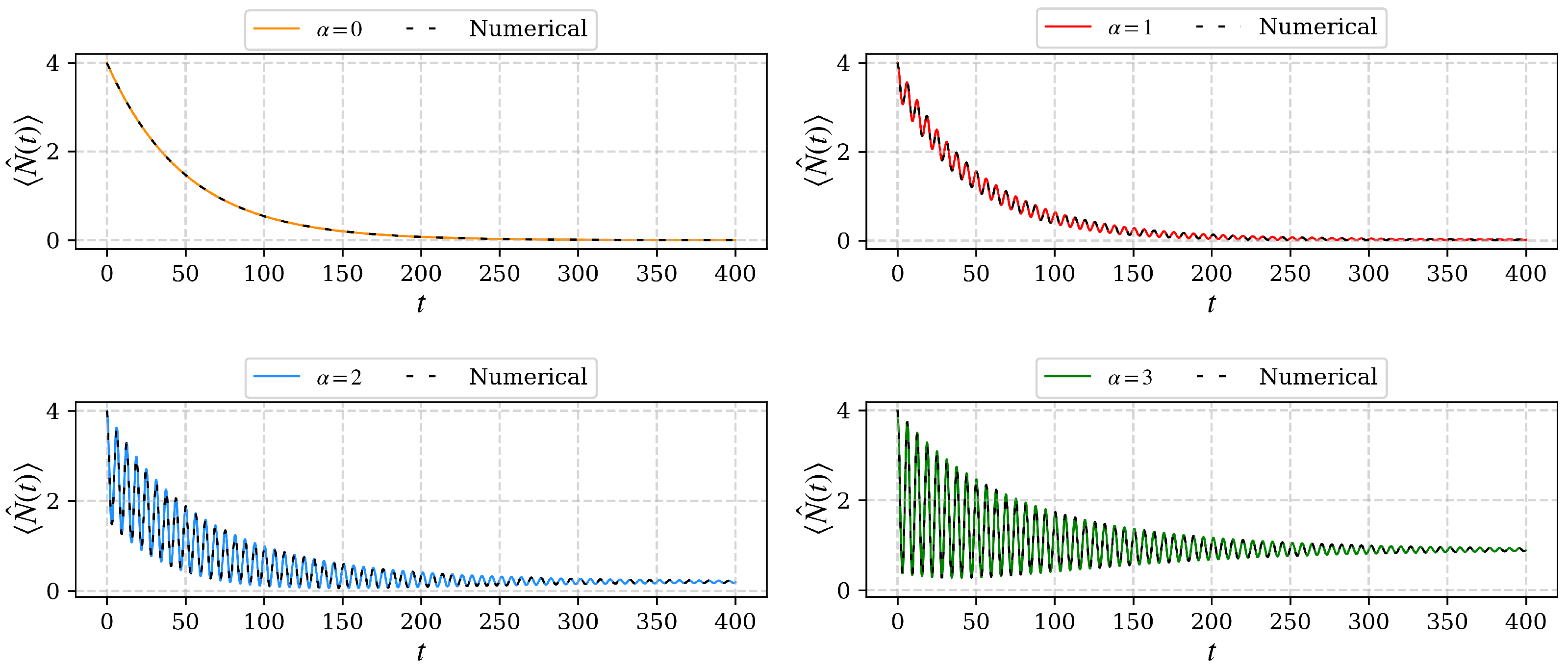
3.3. Coherent States as Initial Conditions

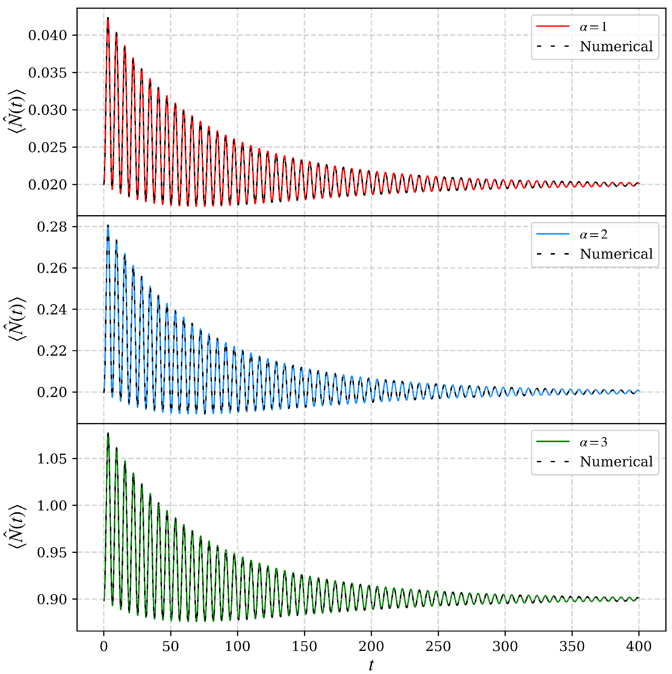
Considering that, initially, both the cavity field and the mechanical oscillator are in coherent states $|\alpha ⟩$ and $|\beta ⟩$, respectively, then, the density operator that describes the initial state of the system is given by $\widehat{\rho }\left(0\right)=|\alpha ⟩⟨\alpha |\otimes |\beta ⟩⟨\beta |$. In this way, it is found that

$$\widehat{W}\left(0\right)=e^{f{\widehat{J}}_{-}}{e}^{g{\widehat{J}}_{+}}{e}^{{\displaystyle \frac{\widehat{J}}{2}}}\widehat{\rho }\left(0\right)=e^{{\left|\beta \right|}^2}{e}^{-{\displaystyle \frac{{\left|\alpha \right|}^2}{2}}\left(2-|e^{g{\beta }^{*}}{|}^2-{\left|e^{f^{*}{\beta }^{*}}\right|}^2\right)}|\alpha e^{g{\beta }^{*}}⟩⟨\alpha e^{f^{*}{\beta }^{*}}|\otimes |\beta ⟩⟨\beta |.$$

(31)

Considering that $\chi$, $\nu$, $\gamma$$\in \mathbb{R}$ then $g=f^{*}$, so it will follow that

$$\widehat{W}\left(0\right)=e^{{\left|\beta \right|}^2-{\left|\alpha \right|}^2\left(1-|e^{g{\beta }^{*}}{|}^2\right)}|\alpha e^{g{\beta }^{*}}⟩⟨\alpha e^{g{\beta }^{*}}|\otimes |\beta ⟩⟨\beta |.$$

(32)

In order to calculate the result of applying $e^{{\widehat{H}}_{1}t}$ and $e^{{\widehat{H}}_{2}t}$ to $\widehat{W}\left(0\right)$, we note the following: By expressing the coherent state of the field in terms of its corresponding Fock states, we find that

$$e^{{\widehat{H}}_{1}t}|\alpha e^{g{\beta }^{*}},\beta ⟩=\sqrt{\xi }exp\left[-{\displaystyle \frac{{\left|\beta \right|}^2}{2}}+{\displaystyle \frac{{\left|\alpha \right|}^2}{2}}\left(1-|e^{g{\beta }^{*}}{|}^2\right)\right]\sum _{k=0}^{\infty }{\theta }_k|k,{\tilde{\beta }}_k⟩,$$

(33)

where $|k⟩$ are the number states of the field, $|{\tilde{\beta }}_k⟩=|{\alpha }_{3}k+\beta e^{{\alpha }_1}⟩$ are the coherent states of the mirror,

$$\xi =exp\left(-{\left|\alpha \right|}^2+{\left|\beta e^{{\alpha }_1}\right|}^2\right),$$

(34)

and

$${\theta }_k={\displaystyle \frac{{\alpha }^k}{\sqrt{k!}}}exp\left[(g{\beta }^{*}+\beta {\alpha }_2{e}^{{\alpha }_1}+\beta {\alpha }_3^{*}{e}^{{\alpha }_1}-iIm\left(\beta {\alpha }_3^{*}{e}^{{\alpha }_1}\right))k\right]exp\left[\left({\displaystyle \frac{|{\alpha }_3{|}^2}{2}}+{\alpha }_4\right)k^2\right].$$

(35)

Then, given that ${\widehat{H}}_1={\widehat{H}}_2^{†}$, we obtain that

$$\widehat{\rho }\left(t\right)=e^{-{\displaystyle \frac{\widehat{J}}{2}}}{e}^{-g{\widehat{J}}_{+}}{e}^{-f{\widehat{J}}_{-}}\left[e^{{\displaystyle \frac{2{\chi }^2\gamma }{{\nu }^2+{\gamma }^2}}t{\widehat{J}}_{\widehat{n}}}\xi \sum _{k=0}^{\infty }\sum _{l=0}^{\infty }{\theta }_k{\theta }_l^{*}|k,{\tilde{\beta }}_k⟩⟨l,{\tilde{\beta }}_l|\right].$$

(36)

By applying the corresponding superoperators, it is found that the density operator of the composite system is given by

$$\widehat{\rho }\left(t\right)=\xi \sum _{k=0}^{\infty }\sum _{l=0}^{\infty }exp\left[{\displaystyle \frac{2{\chi }^2\gamma }{{\nu }^2+{\gamma }^2}}klt-{\tilde{\beta }}_k{\tilde{\beta }}_l^{*}-g^{*}l{\tilde{\beta }}_k-gk{\tilde{\beta }}_l^{*}\right]{\theta }_k{\theta }_l^{*}|k⟩⟨l|\otimes |{\tilde{\beta }}_k⟩⟨{\tilde{\beta }}_l|.$$

(37)

We have considered a coherent pure state as the initial state of the mirror; however, an arbitrary state can also be addressed, as any density operator can be expressed as an integral over projection operators onto coherent states through the Glauber–Sudarshan P representation [20]. Consequently, the evolution of an arbitrary state can be determined by leveraging the known evolution of a coherent state.

Using the explicit form for the functions ${\alpha }_{1,2,3,4}\left(t\right)$ and with $\beta ={\beta }_x+i{\beta }_y$, we obtain the average number of photons

$$⟨\widehat{n}\left(t\right)⟩=\xi \sum _{l=0}^{\infty }exp\left[{\displaystyle \frac{2{\chi }^2\gamma }{{\nu }^2+{\gamma }^2}}t{l}^2-{\left|{\tilde{\beta }}_l\right|}^2-2lRe\left\{g^{*}{\tilde{\beta }}_l\right\}\right]|{\theta }_l{|}^{2}l={\left|\alpha \right|}^2,$$

(38)

and the average number of phonons

$$\begin{array}{cc}\hfill ⟨\widehat{N}\left(t\right)⟩=& \xi \sum _{l=0}^{\infty }exp\left[{\displaystyle \frac{2{\chi }^2\gamma }{{\nu }^2+{\gamma }^2}}t{l}^2-{\left|{\tilde{\beta }}_l\right|}^2-2lRe\left\{g^{*}{\tilde{\beta }}_l\right\}\right]|{\theta }_l{|}^2{\left|{\tilde{\beta }}_l\right|}^2\hfill \end{array}$$

(39)

$$\begin{array}{cc}\hfill =& {\left|\beta \right|}^2{e}^{-2\gamma t}+|{\alpha }_3{|}^2{\left|\alpha \right|}^4+\left(|{\alpha }_3{|}^2+2Re\left\{\beta {\alpha }_3^{*}{e}^{-(\gamma +i\nu )t}\right\}\right){\left|\alpha \right|}^2,\hfill \end{array}$$

(40)

where

$$\begin{array}{c}\hfill |{\alpha }_3{|}^2={\displaystyle \frac{{\chi }^2}{{\nu }^2+{\gamma }^2}}\left(1-2e^{-\gamma t}cos\left(\nu t\right)+e^{-2\gamma t}\right),\end{array}$$

and

$$\begin{array}{c}2Re\left\{\beta {\alpha }_3^{*}{e}^{-(\gamma +i\nu )t}\right\}={\displaystyle \frac{2\chi }{{\nu }^2+{\gamma }^2}}\left[({\beta }_x\nu +{\beta }_y\gamma )\left(e^{-\gamma t}cos\left(\nu t\right)-e^{-2\gamma t}\right)\right.\hfill \\ \hfill \left.+({\beta }_y\nu -{\beta }_x\gamma )e^{-\gamma t}sin\left(\nu t\right)\right].\end{array}$$

We observe that the average photon number in the cavity remains unchanged, as expected, given that only the mirror’s damping is considered. Meanwhile, the average number of phonons depends on both the mean photon number in the cavity and its square, ${\left|\alpha \right|}^4$. In general, we observe a damped oscillatory behavior due to the appearance of decaying exponentials, $e^{-\gamma t}$, multiplied by periodic functions. In the limit $\gamma t\to \infty$, we have that

$$⟨\widehat{N}⟩={\displaystyle \frac{{\chi }^2}{{\nu }^2+{\gamma }^2}}⟨{\widehat{n}}^2⟩={\displaystyle \frac{{\chi }^2}{{\nu }^2+{\gamma }^2}}{\left(\right|\alpha |}^4+{\left|\alpha \right|}^2),$$

(41)

that is, the average phonon number, in general, does not tend to zero. This can be understood as follows: while damping from the reservoir reduces the phonon number, the continuous displacement of the mirror, arising from the interaction term in the Hamiltonian (5), counteracts this effect, leading to oscillations that gradually decay but never fully vanish.

In Figure 2, the time evolution of the phonon number of the mechanical oscillator is shown when the initial state of the mirror is a coherent state with $\beta =2$, for different values of the coherent state amplitude of the field $\alpha$, where $\nu =1$, $\chi =0.1$, and $\gamma =0.01$. The solid colored lines represent the analytical results from Equation (40), while the dashed curves correspond to the numerical solutions of the master Equation (8).

Figure 2. Temporal evolution of the average phonon number with an initial amplitude of the coherent state of the mirror $\beta =2$ with parameters $(\nu ,\chi ,\gamma )=(1.0,0.1,0.01)$ for different values of the amplitude of the coherent state of the field $\alpha$. The analytical results, obtained from Equation (40), are represented by solid colored lines, while the dashed curves correspond to the numerical solutions of the master Equation (8).

Figure 3 illustrates the specific case in which the initial state of the mechanical oscillator is given by the square root of the phonon number from Equation (41). As a consequence, in the limit $\gamma t\to \infty$, the system recovers the initial phonon number. That is, even though the mechanical oscillator is coupled to the environment, the initial phonon number can be recovered under appropriate initial conditions. This behavior is shown for different values of the coherent state amplitude of the field $\alpha$, with parameters $\nu =1$, $\chi =0.1$, and $\gamma =0.01$. The solid lines represent the analytical results, while the dashed curves depict the numerical solutions.

Figure 3. Temporal evolution of the average phonon number when the initial state of the mechanical oscillator is given by the square root of the phonon number in Equation (41) for different values of the amplitude of the coherent state of the field $\alpha$, with parameters $(\nu ,\chi ,\gamma )=(1.0,0.1,0.01)$. The analytical results, obtained from Equation (40), are depicted by solid colored lines, whereas the dashed curves represent the numerical solutions of the master Equation (8).

It is worth noting that for a lossless optomechanical system, $\gamma =0$, we obtain the same results reported in [21] for the average phonon number

$$\begin{array}{c}⟨\widehat{N}⟩={\left|\beta \right|}^2+{\left({\displaystyle \frac{2\chi }{\nu }}\right)}^2{sin}^2\left({\displaystyle \frac{\nu t}{2}}\right){\left|\alpha \right|}^4\hfill \\ \hfill +\left[\left({\left({\displaystyle \frac{2\chi }{\nu }}\right)}^2-{\displaystyle \frac{4\chi }{\nu }}{\beta }_x\right){sin}^2\left({\displaystyle \frac{\nu t}{2}}\right)+{\displaystyle \frac{2\chi }{\nu }}{\beta }_{y}sin\left(\nu t\right)\right]{\left|\alpha \right|}^2.\end{array}$$

(42)

3.4. Steady State

A steady-state solution to Equation (8) may be obtained by assuming that the cavity field is in the Fock state $|k⟩$, while the mechanical oscillator occupies a state $|{\psi }_s⟩$, to be determined under the condition ${\displaystyle \frac{d\widehat{\rho }}{dt}}=0$. Consequently, the system’s density operator is given by

$${\widehat{\rho }}_s=|k⟩⟨k|\otimes |{\psi }_s⟩⟨{\psi }_s|,$$

(43)

where, by substituting (43) into the master Equation (8), we obtain

$$|k⟩⟨k|\otimes \left\{-i\left[\nu \widehat{N}-\chi k(\widehat{b}+{\widehat{b}}^{†}),|{\psi }_s⟩⟨{\psi }_s|\right]+\gamma \mathcal{L}\left[\widehat{b}\right]|{\psi }_s⟩⟨{\psi }_s|\right\}=0.$$

(44)

To solve this equation, we apply the following transformation

$$|{\psi }_s⟩⟨{\psi }_s|={\widehat{D}}_{\widehat{b}}\left({\beta }_k\right)|{\phi }_s⟩⟨{\phi }_s|{\widehat{D}}_{\widehat{b}}^{†}\left({\beta }_k\right),$$

(45)

where, by choosing ${\beta }_k={\displaystyle \frac{\chi k}{{\nu }^2+{\gamma }^2}}(\nu +i\gamma )$, we obtain an equation in which the term $(\widehat{b}+{\widehat{b}}^{†})$ is eliminated, yielding

$$|k⟩⟨k|\otimes \left\{-i\left[\nu \widehat{N},|{\phi }_s⟩⟨{\phi }_s|\right]+\gamma \mathcal{L}\left[\widehat{b}\right]|{\phi }_s⟩⟨{\phi }_s|\right\}=0,$$

(46)

and this equation is satisfied if $|{\phi }_s⟩=|0⟩$. Therefore, in the original frame, it is found that the density operator that makes the system stationary is

$${\widehat{\rho }}_s=|k⟩⟨k|\otimes |{\beta }_k⟩⟨{\beta }_k|,$$

(47)

where $|{\beta }_k⟩$ is a coherent state. Furthermore, we note that the average number of phonons is

$$⟨{\widehat{N}}_k⟩={\displaystyle \frac{{\chi }^2}{{\nu }^2+{\gamma }^2}}{k}^2.$$

(48)

The above value is independent of the initial average number of phonons, as expected. We should stress that although Equation (47) is not the more general steady state solution of the master equation, it is consistent with the result given in (41).

4. Conclusions

We have given a superoperator solution to the master equation that describes the interaction between a quantized field and a moving mirror. Unlike the solution given by Bose et al. [13], our solution allows any initial wavefunction of the combined system. We also presented a steady state solution of the master equation that provides consistent results with the average number of phonons at $\gamma t\to \infty$.

References

1. Aspelmeyer, M.; Meystre, P.; Schwab, K. Quantum optomechanics. Phys. Today 2012, 65, 29–35. [Google Scholar] [CrossRef]
2. Meystre, P. A short walk through quantum optomechanics. Ann. Der Phys. 2013, 525, 215–233. [Google Scholar] [CrossRef]
3. Bowen, W.P.; Milburn, G.J. Quantum Optomechanics; CRC Press: Boca Raton, FL, USA, 2015. [Google Scholar]
4. Aspelmeyer, M.; Kippenberg, T.J.; Marquardt, F. Cavity optomechanics. Rev. Mod. Phys. 2014, 86, 1391–1452. [Google Scholar]
5. Marquardt, F.; Girvin, S.M. Optomechanics. Physics 2009, 2, 40. [Google Scholar] [CrossRef]
6. Metcalfe, M. Applications of cavity optomechanics. Appl. Phys. Rev. 2014, 1, 031105. [Google Scholar]
7. Schliesser, A.; Rivière, R.; Anetsberger, G.; Arcizet, O.; Kippenberg, T.J. Resolved-sideband cooling of a micromechanical oscillator. Nat. Phys. 2008, 4, 415–419. [Google Scholar]
8. Chan, J.; Alegre, T.P.M.; Safavi-Naeini, A.H.; Hill, J.T.; Krause, A.; Gröblacher, S.; Aspelmeyer, M.; Painter, O. Laser cooling of a nanomechanical oscillator into its quantum ground state. Nature 2011, 478, 89–92. [Google Scholar] [PubMed]
9. Brooks, D.W.; Botter, T.; Schreppler, S.; Purdy, T.P.; Brahms, N.; Stamper-Kurn, D.M. Non-classical light generated by quantum-noise-driven cavity optomechanics. Nature 2012, 488, 476–480. [Google Scholar] [PubMed]
10. Teufel, J.D.; Donner, T.; Castellanos-Beltran, M.A.; Harlow, J.W.; Lehnert, K.W. Nanomechanical motion measured with an imprecision below that at the standard quantum limit. Nat. Nanotechnol. 2009, 4, 820–823. [Google Scholar] [CrossRef] [PubMed]
11. Bemani, F.; Roknizadeh, R.; Naderi, M.H. Theoretical scheme for the realization of the sphere-coherent motional states in an atom-assisted optomechanical cavity. J. Opt. Soc. Am. B 2015, 32, 1360–1368. [Google Scholar] [CrossRef]
12. Mancini, S.; Man’Ko, V.I.; Tombesi, P. Ponderomotive control of quantum macroscopic coherence. Phys. Rev. A 1997, 55, 3042. [Google Scholar] [CrossRef]
13. Bose, S.; Jacobs, K.; Knight, P.L. Preparation of nonclassical states in cavities with a moving mirror. Phys. Rev. A 1997, 56, 4175. [Google Scholar]
14. Ventura-Velázquez, C.; Rodríguez-Lara, B.M.; Moya-Cessa, H.M. Operator approach to quantum optomechanics. Phys. Scr. 2015, 90, 068010. [Google Scholar] [CrossRef]
15. Arévalo-Aguilar, L.M.; Moya-Cessa, H.M. Cavidad con pérdidas: Una descripción usando superoperadores. Rev. Mex. Física 1995, 42, 675–683. [Google Scholar]
16. Phoenix, S.J. Wave-packet evolution in the damped oscillator. Phys. Rev. A 1990, 41, 5132. [Google Scholar]
17. Law, C.K. Interaction between a moving mirror and radiation pressure: A Hamiltonian formulation. Phys. Rev. A 1995, 51, 2537. [Google Scholar] [CrossRef]
18. Primo, A.G.; Pinho, P.V.; Benevides, R.; Gröblacher, S.; Wiederhecker, G.S.; Alegre, T.P.M. Dissipative Optomechanics in High-Frequency Nanomechanical Resonators. Nat. Commun. 2023, 14, 5793. [Google Scholar] [CrossRef]
19. Mancini, S.; Tombesi, P. Quantum noise reduction by radiation pressure. Phys. Rev. A 1994, 49, 4055. [Google Scholar] [CrossRef] [PubMed]
20. Glauber, R.J. Coherent and incoherent states of the radiation field. Phys. Rev. 1963, 131, 2766. [Google Scholar] [CrossRef]
21. Medina-Dozal, L.; Récamier, J.; Moya-Cessa, H.M.; Soto-Eguibar, F.; Román-Ancheyta, R.; Ramos-Prieto, I.; Urzúa, A.R. Temporal evolution of a driven optomechanical system in the strong coupling regime. Phys. Scr. 2023, 99, 015114. [Google Scholar]
22. Wei, J.; Norman, E. On global representations of the solutions of linear differential equations as a product of exponentials. Proc. Am. Math. Soc. 1964, 15, 327–334. [Google Scholar] [CrossRef]