Article

Quantum Computation of the Cobb–Douglas Utility Function via the 2D Clairaut Differential Equation

by
Isabel Cristina Betancur-Hinestroza
1,*,
Éver Alberto Velásquez-Sierra
2,
Francisco J. Caro-Lopera
2 and
Álvaro Hernán Bedoya-Calle
3
1
Faculty of Economic Sciences, University of Medellin, Cra. 87 # 30-65, Medellín 050026, Colombia
2
Faculty of Basic Sciences, University of Medellin, Cra. 87 # 30-65, Medellín 050026, Colombia
3
Independent Researcher, Cra 86 # 30-12, Medellín 050026, Colombia
*
Author to whom correspondence should be addressed.
Quantum Rep. 2025, 7(1), 1; https://doi.org/10.3390/quantum7010001
Submission received: 27 November 2024 / Revised: 16 December 2024 / Accepted: 21 December 2024 / Published: 29 December 2024

Abstract

:
This paper introduces the integration of the Cobb–Douglas (CD) utility model with quantum computation using the Clairaut-type differential formula. We propose a novel economic–physical model employing envelope theory to establish a link with quantum entanglement, defining emergent probabilities in the optimal utility function for two goods within a given expenditure limit. The study explores the interaction between the CD model and quantum computation, emphasizing system entropy and Clairaut differential equations in understanding utility’s optimal envelopes. Algorithms using the 2D Clairaut equation are introduced for the quantum formulation of the CD function, showcasing representation in quantum circuits for one and two qubits. Our findings, validated through IBM-Q simulations, align with the predictions, demonstrating the robustness of our approach. This methodology articulates the utility–budget relationship through envelope representation, where normalized intercepts signify probabilities. The precision of our results, especially in modeling quantum entanglement, surpasses that of IBM-Q simulations, which require extensive iterations for similar accuracy.

1. Introduction

Quantum computation influences a broad range of knowledge areas, including materials science [1], optimization [2], photonics [3,4], and medicine [5]. Economic theory benefits from physics, particularly through particle models, to comprehend complex structures. This method, borrowed from physics to address economic challenges, is known as econophysics. It notably incorporates quantum physics and thermodynamics to explore economic phenomena [6].
The study of economics revolves around two primary pillars: microeconomics and macroeconomics. Microeconomics examines the behaviors of individual economic agents, while macroeconomics considers these behaviors in aggregate. Within these traditional models, one of the key theoretical tools is the Cobb–Douglas function [7]. This function originated from a least-squares exercise aimed at estimating manufacturing output in the United States between 1899 and 1922.
This exercise led to a formula that represents a production function for systems with two factors: labor (L), quantified by the average number of employees, and capital (K), measured through estimated annual changes in manufacturing’s fixed capital. Additionally, α and β represent the elasticities of production in response to variations in labor and capital, respectively. A is identified as the total factor productivity, highlighting the model’s need for adjustable parameters to accurately reflect production dynamics.
This version of the function effectively addresses production issues within the framework of profit maximization, a core principle of corporate theory. Its application aligns with the neoclassical postulate of economic rationality found in consumer theory. Tracing back to the utilitarian model proposed by the marginalists, particularly Bentham, the Cobb–Douglas function has also served to depict the utility function, focusing on the consumption of two types of goods.
The Cobb–Douglas function plays a crucial role in assessing the influence of inputs on cassava production, optimizing factors like human labor, fertilizers, chemicals, and seeds [8,9]. From 1990 to 2017, it has marked the economic efficiency of countries in the Americas and the Caribbean [10]. Similarly, it has analyzed key factors in Pasaran mussel production levels and the efficiency of tool and material use in cultivation. Other studies have examined four variables: the number of bamboos (X1), straps (X2), grouper (X3), and labor (X4) [11].
The Cobb–Douglas function is fundamentally a tool for data fitting. Within the context of entropy, it offers a superior fit for production data and incurs lower costs than the benchmark function. Optimization through the Lagrangian method necessitates knowledge of factor prices. However, when integrating entropy into the Lagrange framework, these specific parameters are not required.
Optimization processes are typically used in scenarios limited by information on the prices of goods and income, particularly for utility functions, and by the prices of production factors and budget constraints. However, if the goal is to evaluate the possible set of tangents to a specific production or utility function, more advanced techniques are needed. Among these, the Clairaut equation stands out, not requiring significantly greater computational resources for effective implementation.
Recent research highlights the use of quantum descriptions in economic applications within markets. Recognizing quantum science’s capacity to distinguish between the observed phenomena and the observer, one study proposes applying quantum game theory to economics [12]. Similarly, another analysis delves into quantum negotiation games, avoiding institutional trade-offs, a concept prevalent in social sciences [13]. Additionally, a particular study adopts this approach to explore the dynamics of English quantum auctions [14].
A study by Pawela and Sładkowski (2013) [15] employs the prisoner’s dilemma game to model strategic interactions among three players using quantum tools. More broadly, ref. [16] offer a comprehensive overview of game theory from a quantum computing perspective. This approach significantly expands the range of decision-making possibilities within this economic study area.
In this study, we aim to quantize economic processes using an explicit function derived from envelopes, which we then compare with quantum circuit outcomes. This involves the Cobb–Douglas utility function under the constraint of nominal income, explored in two specific scenarios: (i) when the nominal income (m) equals 1, corresponding to optimal utility function choices, and (ii) when the nominal income (m) is less than 1, pertaining to savings behavior.
We present the implementation of single-qubit quantum circuits for condition (i), focusing on calculating the envelopes. At the tangency points and intercepts, we compute the entropy. For condition (ii), our approach builds on the envelopes derived in condition (i). We then plot lines that fall below the constraint (m < 1), employing two qubits for this specific analysis.
This paper introduces a novel method to briefly state the method’s purpose, e.g., analyzing consumer choices, modeling economic behavior. While we illustrate our approach using a specific parameterization of the Cobb–Douglas utility function, the methodology is designed for broad applicability beyond this particular instance. Several key features ensure this generality:
  • Our method is grounded in the Clairaut differential equation, a general framework for describing function envelopes. This foundation is independent of specific functional forms or parameter values, providing a robust basis for analyzing tangency relationships between curves. The method for obtaining tangent points, intercepts, and the associated probabilities is derived from the general solution of the Clairaut equation, thus applying universally to any parameter set.
  • Our mapping of economic concepts to the quantum realm relies on interpreting probabilities through the canonical budget equations and the geometric properties of envelopes. This translation is independent of specific Cobb–Douglas parameters. We demonstrate how key geometric features, such as intercepts and tangency points (which are parameter dependent), can be mapped to probabilities within this quantum framework. Consequently, our calculations are applicable to any parameterization of the Cobb–Douglas utility function.
  • The homogeneity of the Cobb–Douglas function allows for rescaling the budget and parameters without affecting the core results. Our analysis utilizes normalized quantities that remain invariant under such rescaling, ensuring that our findings are representative beyond the specific values used for demonstration. Furthermore, our method emphasizes the structural properties of the utility function and budget constraint, particularly the tangency relationships captured by the Clairaut equation. The focus is on general characteristics, like the interplay between prices, income, and consumption choices, rather than specific numerical values.
  • While the Cobb–Douglas function serves as a useful example, it is well established in econometrics and captures essential behaviors in consumer and production theory. Our methodology extends to a broader class of concave, well-behaved utility and production functions. The underlying economic concepts (e.g., tangency of indifference curves and budget constraints, elasticity, and marginal rates of substitution) can be represented within our quantum formalism, further supporting the general applicability of our approach.
  • This paper presents an initial instantiation of our method. Future work will explore a wider range of parameters and functional forms through further simulations and empirical analysis, providing additional validation of its generality and robustness.
Our method’s generality stems from its foundation in general mathematical principles, its parameter-independent quantum mapping, its focus on structural properties, and its grounding in established economic theory. The specific case presented here serves primarily as an illustrative example of the broader applicability of the proposed framework.

2. Simulation and Methods

The Cobb–Douglas utility function, defined as
u = k x α y β
is subject to the constraint m = p x x + p y y , where m represents nominal income, and px, and py are the prices of goods x and y, respectively. By reformulating the utility function to maximize it under this constraint, we derive the expressions for the optimal consumption of goods x and y. Specifically, the optimal quantity of x is determined as
x = α m p x α + β
and for y, by substituting x’s optimal value into the budget constraint, we find
y = β m p y α + β
Consequently, the optimal utility, achieved by evaluating the optimal consumption values of x and y, simplifies to
u = k m α + β α α β β p x α p y β α + β α + β
encapsulating the utility maximization process within the Cobb–Douglas framework under the given economic conditions.

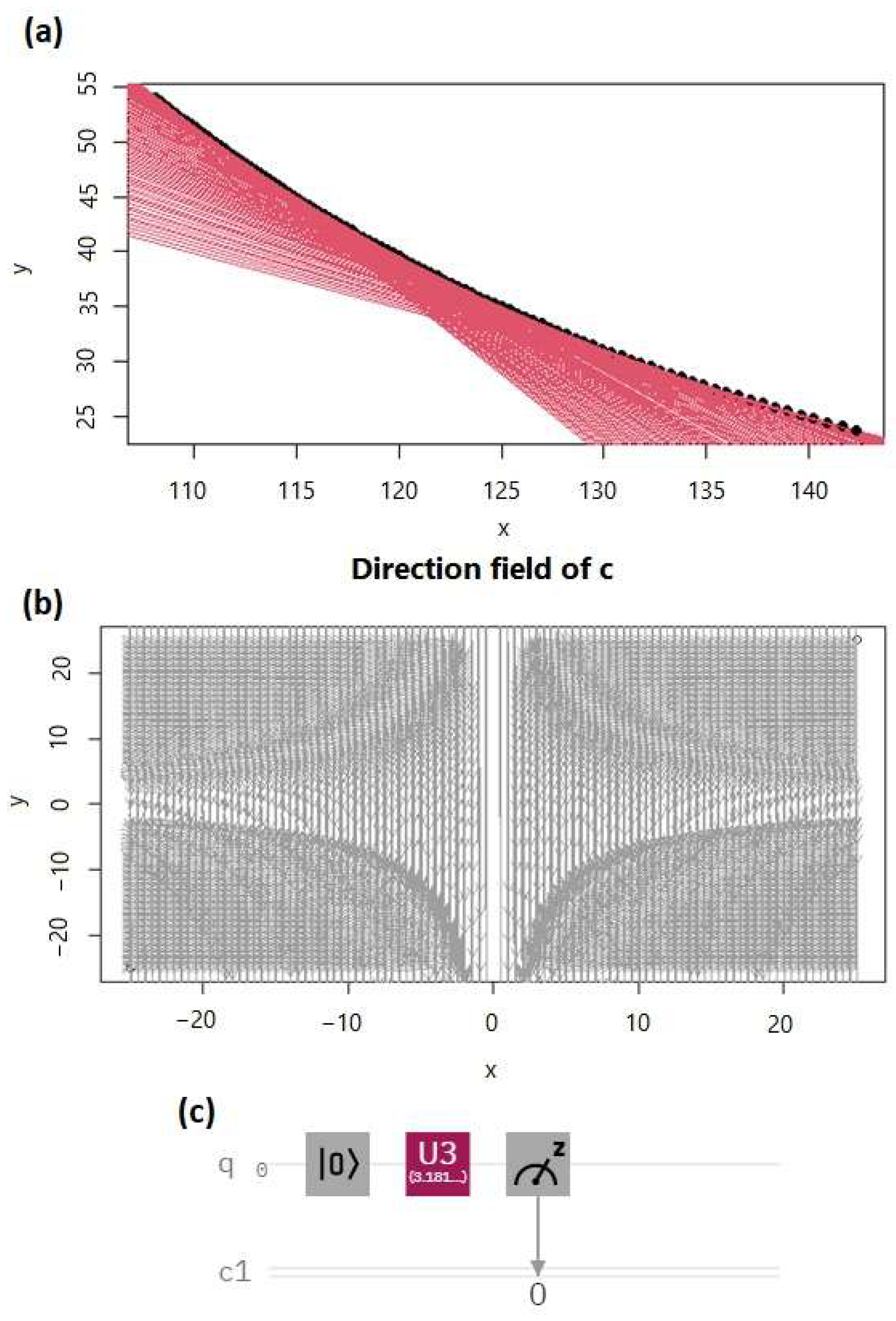
Envelopes of the Cobb–Douglas Function

By expressing Equation (1) in terms of y, we arrive at the following equation:
y = k 1 x α u 1 / β
From this, we calculate the slope y x , representing the marginal product of production, resulting in the following equation:
y x = k 1 β u 1 β x 1 α β α β = c
Solving for x gives us:
x = c k 1 β u 1 β β α β α + β
Substituting (7) into (5) yields the ordinate of the tangency point, expressed as the following equation:
y t c = c α α + β k 1 α + β u 1 α + β α α α + β β α α + β
Furthermore, substituting (7) and (8) into the general solution of the Clairaut equation y = c x + f c leads to the following equation:
f c = c α α + β k 1 α + β u 1 α + β α α α + β β β α + β α + β
Differentiating (9) with respect to c to find f’(c) results in the following equation:
f c = c 1 + α α + β k 1 α + β u 1 α + β α 1 α α + β β β α + β
From the singular solution of the Clairaut differential equation, 0 = x t + f c , we determine the abscissa of tangency, shown in the following equation:
x t c = f c
The x-intercept and y-intercept are then obtained as in Equations (12) and (13), respectively:
x i c = c 1 f c
y i = f c

3. Results and Discussion

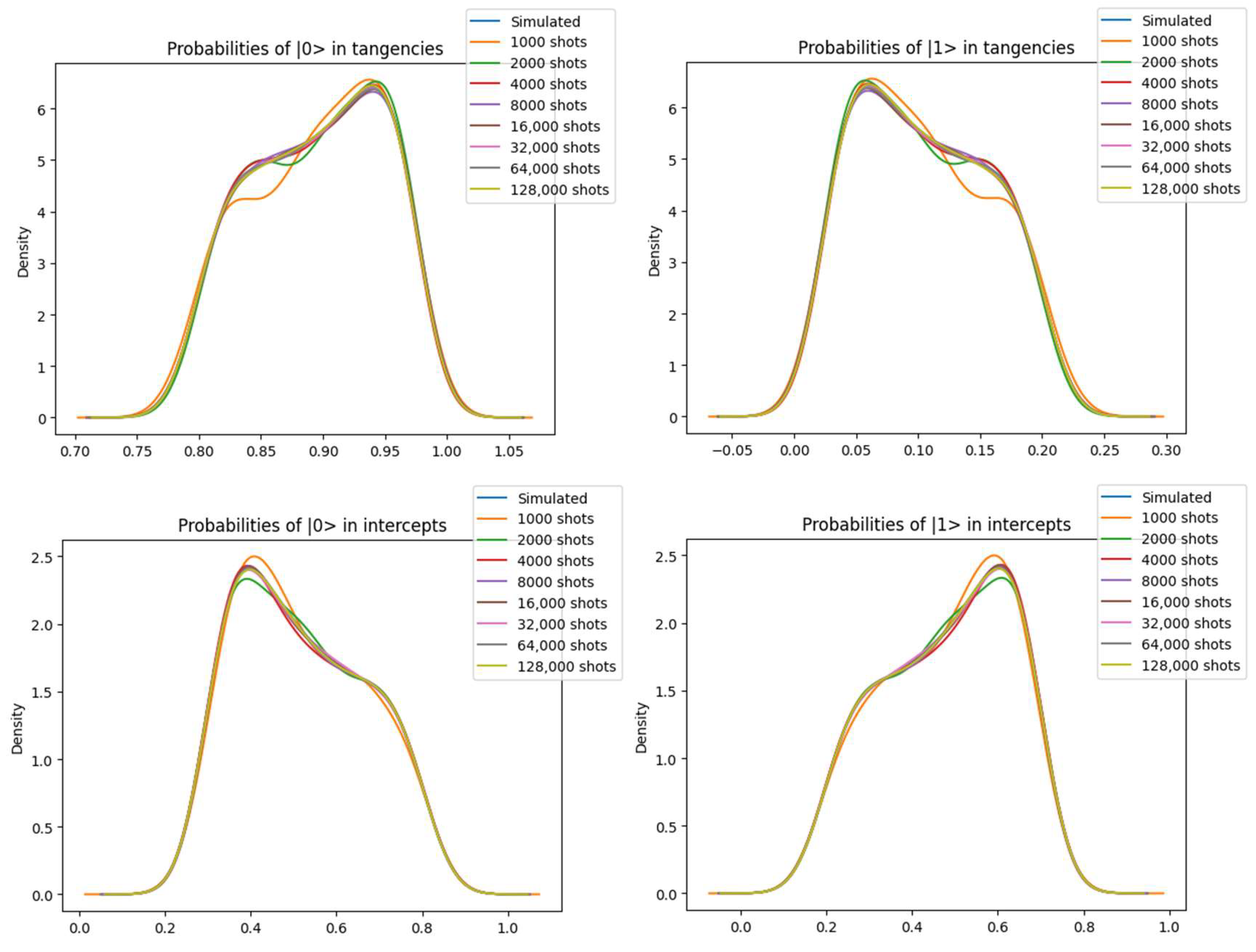
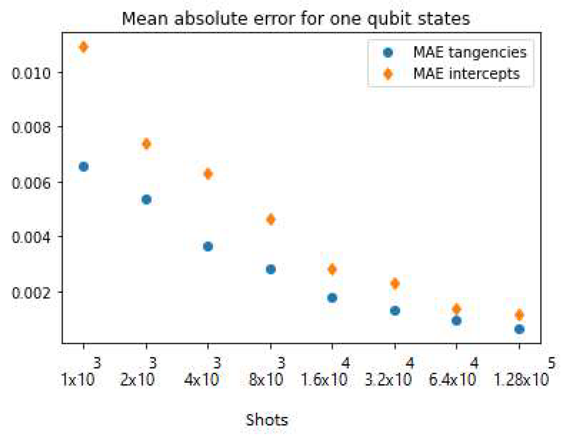
3.1. Calculation of the Probabilities of the Cobb–Douglas Function for a Qubit (q0)

The general state of a qubit is defined by ψ = α q 0 0 + β q 0 1 , where the column vectors define the states 0 = 1 0 and 1 = 0 1 ; furthermore, α q 0 and β q 0 are complex numbers, and their squared norms are interpreted as probabilities. Where α q 0 2 is the probability of finding the qubit in state 0 , β q 0 2 represents the probability of finding the qubit in state 1 . The entanglement of the probabilities is given by the following relationship: α q 0 2 + β q 0 2 = 1 .
The canonical equation of the line is given by
y b + x a = 1
where a and b are intercepts of the line with x and y, respectively. The following functional relationships define the probabilities for a qubit:
α q 0 2 = a 2 r 2 = P 1 β q 0 2 = b 2 r 2 = P 2
with r = a 2 + b 2 .
From the restriction m = p x x + p y y , we obtain the intercepts: when x = 0 , we have y = m p y ; when y = 0 , we have x = m p x , and the budget set is defined, in this case, as p x x m + p y y m = 1 . The canonical equation of the line is given by y m p y + x m p x = 1 , and the probabilities on the intercepts are given by Equation (15):
α q 2 = m p y 2 r 2 β q 2 = m p x 2 r 2
with r = m p y 2 + m p x 2 .
A generalization of the representation of the Cobb–Douglas function for a qubit is Equations (5)–(10), being derived from the Clairaut differential equation that considers the utility function as a parameter, and all the possible optima that define the envelopes deprecates Equation (16). The canonical equation in terms of the intercepts in the envelopes, Equations (12) and (13), is as follows:
y f c + x c 1 f c = y y i c + x x i c = 1
whose probabilities are given by:
α q 2 = x i c 2 r i 2 β q 2 = y i c 2 r i 2
with r i = y i c 2 + x i c 2 .
It is possible to calculate the intermediate probabilities at the points of tangency using the envelope lines, offering an entangled probability for a qubit; in this context, Equations (17) and (18) in the canonical line equation produce interlocked probabilities, where both the percentages of one product and the other are determined.
We will compare the explicit model obtained from the envelopes and the one implemented in a quantum circuit; we use the gate U3 applied to the state 0 :
U 3 0 = c o s θ 2 e i λ s i n θ 2 e i λ s i n θ 2 e i λ + ϕ c o s θ 2 1 0
U 3 0 = c o s θ 2 e i λ s i n θ 2 ,
where the angle θ in the range (0, 1] can be determined with the following relationship:
c o s θ 2 e i λ s i n θ 2 = P 1 0 + P 2 1 = P 1 P 2
So, θ = 2 c o s 1 P 1 .

3.2. Scaling Economic Parameters and Its Implications in the Quantum Circuit

As can be seen in Figure 1, scaling economic parameters directly affects the quantum circuit model. This occurs in the following ways:
Nominal income (m): An increase in m represents a relaxed budget constraint. This is reflected in the quantum circuit by altering the coefficients related to the intercepts in Equation (17), since these depend on the budget (m) and prices (px and py). The angles θ1 and θ2, which determine the probabilities associated with each measurement outcome (Equations (30) and (31)), are modified when the parameters change. A larger m leads to greater probabilities in the spending regime than in the saving regime, implying an altered entanglement. Prices (px and py): Changes in prices will alter the intercepts, as described by Equations (12) and (13). When prices of goods change, the angles and probabilities of the qubits are modified. A change in the prices alters the trade-offs and, thus, the optimal choices, as reflected in different quantum probabilities. Utility function parameters (α and β): Modifying the parameters α and β of the utility function changes the shape of the utility curve and, thus, changes the slope of the utility function. This will affect the marginal rate of substitution and, thus, changes the tangency points and probabilities.
Using the information from the experimental database [17], we fix the parameters of the Cobb–Douglas function, where k = 1.01, α = 3/4, β = ¼, and nominal income m = 100. The slope c is calculated on the interval (−1.5, −0.5) with a length of m + 1 values (see the Figure 2). The constraint allows us to fix the goods x and y and its price px as an increasing sequence of m + 1 values, whose first value is min 1 x t c , 99 x t c and last value is max 1 x t c , 99 x t c . For the price py, it is calculated as a decreasing sequence of m + 1 values, whose first value is max 1 y t c , 99 y t c and last value is min 1 y t c , 99 y t c . We develop in-house software [18] using the Python programming language [19] for implementing this background model.
In Table S1 of [17], (xo, yo) are the optima of the utility function, obtained with Equations (2) and (3), and (xt, yt) are the points of tangency given by Equations (8) and (11), with the corresponding intercepts xi and yi computed using Equations (12) and (13).
Taking a particular case from Table S1 of [17], with px = 0.429228, py = 1.950558, xo = 174.7322, yo = 12.81684, c = −1, and u = 91.84306, we build the envelopes of the function (see SI in Table S2 of [17]). Then, we calculated the probabilities for the intercepts and tangencies using the circuit (c) in Figure 2. The results can be seen in Table S4 of [17] and Figure 3.
In Figure 4, we added the comparison between the number of shots and the error (MAE) for the tangencies and intercepts, where it can be observed that the error is lower for the tangencies.
Entropy is a utility maximization exercise involving the constraint in a microeconomic environment. However, its importance can also be seen in the economic circuit, where it involves the first and second economic laws, δ P = d K λ d F , where it shows the relationship of production (P), capital (K), and entropy (F). Entropy is a measure of the disorder of a system, and (−dF) means the reduction of disorder. Production means tidying up, putting all parts in order. The monetary value of production depends on the standard of living (λ) [7].
As observed in Figure 5 entropy in the context of the bivariate Cobb–Douglas production function is obtained from all possible scenarios of combinations of the two goods involved and, in our case, the envelopes to said function, both in their tangencies and in intercepts, generate complementary probabilities that can account for said disorder, an aspect that connects the well-known definition of entropy in econophysics with the intrinsic quantum entanglement in the linear budget constraint function.
As observed in [17], Annex A1, under “Row Number” for evaluating the Time/Step, it can be concluded that the consistent decrease in both the tangency and intercept entropy suggests that the system is becoming more structured and predictable.
The intercepts in the Clairaut equation give order to the system insofar as they establish the limits of consumption possibilities imposed by the allocation of prices in the market, and given the preferences represented by the utility function, it is possible to determine an optimal consumption.

3.3. Calculation of the Probabilities of the Cobb–Douglas Function for Two Qubits (q0 and q1)

The complete area under the optimal tangent of the utility curve represents the set of consumption possibilities or all the different combinations of goods without exceeding disposable income. This means that we can consume a value equal to or less than budgeted. Quantum modeling is not considered at values higher than the tangent, since it implies having a higher budget that is not available; therefore, it is not possible to acquire combinations of goods that are higher than the budget.
For considering a budget less than 1 (less than the available budget), we will use two qubits and the vector r on the interval (0, 1] that sweeps the area under the curve with boundaries at intercepts a and b and slope c. The canonical equation of the line is given by y b + x a = r , with r = r 1 , r 2 .
Constructing the system of equations, we have:
y r 1 b + x r 1 a = 1 y r n b + x r n a = 1
Adding in (19), we obtain:
y r 1 b + y r 2 b + + y r n b + x r 1 a + x r 2 a + + x r n a = n
y b 1 r 1 + 1 r 2 + + 1 r n + x a 1 r 1 + 1 r 2 + + 1 r n = n
Rewriting the canonical equation of Expression (21), we have:
y n b i = 1 n 1 r i 1 + x n a i = 1 n 1 r i 1 = 1
The general state of two qubits is given by:
ψ = α q 0 00 + β q 0 01 + φ q 1 10 + δ q 1 11
The moduli of the coefficients in Equation (23) represent the probabilities of determining the entanglement of the qubit states. Considering that UA and UB are two general unitary operators acting on the entanglement of the pair of qubits initialized in the state |00⟩:
ψ f = U A U B 00 = c o s θ 1 2 c o s θ 2 2 c o s θ 1 2 e i ϕ 2 s i n θ 2 2 c o s θ 2 2 e i ϕ 1 s i n θ 1 2 s i n θ 1 2 e i ϕ 1 + ϕ 2 s i n θ 2 2
By demanding that the system of equations in (24) be equal to Equation (23), we can obtain a representation of the equations for the squared moduli of the coefficients.
Both φ q 1 and δ q 1 are auxiliary variables in that α q 0 and β q 0 refer to the quantities of the good x and y, respectively, and whose probabilities can be determined using the canonical Equation (22):
α q 0 2 = n a i = 1 n 1 r i 1 2 R 2 = w 1 β q 0 2 = n b i = 1 n 1 r i 1 2 R 2 = w 2
With R 2 = n a i = 1 n 1 r i 1 2 + n b i = 1 n 1 r i 1 2 , where 0 < w 1 < 1 and 0 < w 2 < 1 , for the effects of the domain of the angles in (0,1], the probabilities will be defined as P 1 = w 1 2 and P 2 = w 2 2 .
By squaring the moduli of the coefficients in Equations (23) and (24) and simplifying, the following system of equations in probabilities with intrinsic normalization is obtained:
P 1 = c o s 2 θ 1 2 c o s 2 θ 2 2
P 2 = c o s 2 θ 1 2 s i n 2 θ 2 2
P 3 = φ q 1 2 = s i n 2 θ 1 2 c o s 2 θ 2 2
P 4 = δ q 1 2 = s i n 2 θ 1 2 s i n 2 θ 2 2
From Equations (26)–(29), we can determine θ 1 and θ 2 as follows:
θ 1 = 2 c o s 1 P 1 + P 2
θ 2 = 2 t a n 1 P 2 P 1
With θ 1 and θ 2 , we calculate P3 and P4 with the trigonometric representation of Equations (28) and (29).
In Figure 6, we can see all lines below the line in the tangency c = −1. The probabilities were calculated in all points of tangencies in Table S2 in [17] only use the values of the intercepts for the envelopes. The model is constructed for the values of intercepts a , b = x i , y i applied in Equations (26)–(31). The comparative outcomes between the model and quantum circuit are shown in Figure 7.
The calculations performed on the quantum computer for each group of shots reveal, in each case, the four probabilities that add up to 1 and correspond to the square of the moduli of the α q 0 , β q 0 , γ q 1 , and δ q 0 coefficients in quantum entanglement. If we denote the probabilities as P1, P2, P3, and P4, respectively, it is shown that P1 and P2 have the same distribution, as well as P3 and P4.
Indeed, it suffices to prove that P1 and P2 (P3 and P4) are linearly related and satisfy the Gauss–Markov theorem. The following table shows the results of the normality test (the test for homoscedasticity and uncorrelatedness of the errors are similarly accepted) (see Table 1 and Table 2):
Not only are the probabilities equal in pairs, but they are complementary at 0.5. Specifically, P 1 + P 3 P 1 + P 4 0.5 and P 2 + P 3 P 2 + P 4 0.5 . To demonstrate this, we first use a test of variances on each group of shots. The results in Table 3 indicate that the variances are equal in all cases, with a high p-value of the test.
A similar result to that in Table 3 is obtained for complementarity with P2, P3, and P4. Once we have shown that the variances are statistically similar, we proceed to calculate the test of equality of means at 0.5 between P1 + P3 and P1 + P4, and the results with a high statistical significance show the same in Table 4.
The complementarity of probabilities at 0.5 between P1 (P2) and P3 or P4 relates the intertwining of spending and saving in a symmetrical way; that is, high probabilities in spending are compensated by low probabilities in saving and vice versa. In the same way, the equality between P1 and P2 (P3 and P4) shows that the probabilities in the entanglement associated with spending or associated with saving have the same contribution in each quantum event but with an imbalance from large to small or vice versa. In our context, the quantum event refers to the interpretation of quantum mechanics that preserves the core probabilistic nature of outcome measurements. These probabilities fundamentally define a system’s states and the measurement process. The results indicate that the probabilities between spending and saving simultaneously run through the whole possible spectrum, i.e., quantum entanglement can explore the full dynamics between spending and saving as expected.

4. Comparative Analysis

The quantum circuit approach offers new possibilities for economic modeling but is not without its challenges. Below, we compare its strengths and limitations with traditional approaches:
Strengths of the quantum approach:
  • Entanglement as a novel tool: The ability to represent economic choices through quantum entanglement is not possible with conventional solutions. This could lead to new insights into complex economic behaviors.
  • Simulation of trade-offs: Quantum mechanics allows for the direct simulation of trade-offs between goods as quantum probabilities within the budget constraint, which has a clear physical interpretation in our model. This provides a more explicit way of modeling the economic trade-offs.
  • Probabilistic nature: The quantum approach allows the system to work with probabilities between combinations of goods, and this allows for a better approach to the system, where probabilities play a crucial role.
  • Non-linearity: The model represents the non-linearity of economic phenomena through its mathematical construction.
Drawbacks and limitations of the quantum approach:
  • Resource intensive: Current quantum computing hardware still presents limits and requires the use of specific platforms (such as IBM-Q). This makes it still a non-conventional approach for modeling utility.
  • Practicality on large scales: While our model presents a quantum computation of utility for two types of goods, real economics studies involve very large scales of goods, and it is not clear how to extend the model for this kind of analysis.
  • Interpretation of quantum probability: While our probabilities have an economic meaning, further study in the subject is needed, since there is still no consensus on interpreting quantum probability.
Comparison with conventional solutions:
  • Conventional solution advantages: direct and computationally less intensive than quantum approaches for optimization and elasticity calculations;
  • Conventional solution limitations: lacks the capability to explicitly model entanglement or probabilistic nature through quantum mechanisms and lacks an underlying physical approach.

5. Conclusions

In this paper, we have expressed the Cobb–Douglas utility model as a differential flow defined by the Clairaut equation. The new model allows us to characterize utility from the theory of envelopes, giving a new meaning to the optimal utility and the linear function of budget availability for the consumption of two types of goods. With the Clairaut model, the tangents and intercepts of the envelopes are translated into complementary probabilities that can be connected to quantum computation theory. The emerging entanglements for one and two qubits allow for the respective quantum modeling of the total available consumption or the savings associated with lower consumption. This new view of an econometric model from a differential flow in its quantum context allows us to further to characterize entropy and to bring the corresponding calculations closer to the modern and fast world of quantum computation.
From the economic–physical point of view, entropy comes from the total number of possible combinations of the consumption of goods represented in the associated Cobb–Douglas utility function. In this paper, we characterize the entropy from the envelopes to the utility function, an aspect that allows us to consider these tangents and intercepts as complementary probabilities emerging from the entanglement that defines the linear function of the budget availability, both with the maximum possible consumption and with the lowest available consumption. Both scenarios are modeled with one and two qubits, respectively. In the latter case, two of the entanglements define the expenditure, and the remaining two are associated with savings, i.e., consumption below the total budget.
The exact expressions derived here for one- and two-qubit quantum entanglements in the econometric context perform more efficiently than calculations from IBM-Q quantum computer simulations, which require a large number of shots to match the exact results.
The results indicate that the probabilities between spending and saving simultaneously run through the whole possible spectrum, i.e., quantum entanglement can explore the whole dynamics between spending and saving as expected.
Finally, we want to add the interesting question:
The selection of this particular case study warrants clarification. What specific criteria motivated its choice, and does it present discernible computational or theoretical advantages over the alternative cases considered?
The choice of this specific case, with the parameters outlined in Table S1 of [17], was primarily driven by the need to provide a concrete and verifiable example for our novel methodology linking the Cobb–Douglas utility function with quantum computation. While it might appear that a specific set of parameters could limit the generality of our approach, we would like to emphasize that this is not the case due to the properties of both the Cobb–Douglas function and the underlying mathematical principles employed in our model.
First, the Cobb–Douglas utility function is a continuous and differentiable function that, by its mathematical nature, allows for the characterization of all of its envelope curves. This means that for any specific set of parameters defining the function, it is always possible to perform the analysis we propose. Our specific case in Table S1 of [17] provides an example where the envelope curves can be calculated explicitly. Our model is general and can be used with other parameters without any problems, but the calculations are difficult to show in a clear way. The main point is that we are using a method that can be applicable to any parameter set, and therefore, we choose a parameter set that allows for numerical calculations.
Second, our model uses the Clairaut equation to characterize the envelope curves in a general manner. While each set of parameters produces specific envelopes, the procedure to determine these envelopes and their tangency and interception points remains the same. That is, the properties that we use to make the analogy between economic and quantum mechanics is totally general, and the specific case is an example.
Specifically regarding the scaling factors, we rely on the property that the Cobb–Douglas function exhibits homogeneity of degree one when considering the case of production (and similar properties for the utility function). As a result, any scaling of the budget constraint (effectively scaling both consumption levels and income by a common factor) does not alter the relative proportions in the equilibrium solution nor the probabilities associated with each consumption choice. Mathematically, this means that the optimal choices and the slopes in the model are not affected by a uniform scaling of income and quantities. This scaling symmetry implies that the probabilities, when calculated in their normalized form, remains constant, regardless of the budget level. This is because it equally affects the intercepts, and when normalized, it vanishes. Thus, any change in the budget, prices, or parameters of the Cobb–Douglas utility function can be analyzed on the quantum mechanical probabilities of the system, independently of the level of consumption. This is a very important point because the main goal of the paper is to relate economic magnitudes with the probabilities on quantum mechanical systems. Our starting point was the simple case of m = 1, but it did not limit the scope of the analysis.
From a computational perspective, this specific set of parameters allowed us to achieve the following:
  • Verify the general nature of the system by showing explicit numerical calculations using an example;
  • Conduct simulations on the IBM-Q quantum platform, which requires a well-defined initial setup; this concrete example served as a crucial validation point for our proposed approach and the associated interpretations.
While our analysis begins with a specific case, it is important to emphasize that the method can be applied to other cases. This initial demonstration has allowed us to illustrate the potential of our approach and paves the way for future research that will systematically explore a broader range of parameters, but this would not add anything to the main idea of the paper, which is to make an analogy between economic and quantum mechanical probabilities.

Author Contributions

Conceptualization, Á.H.B.-C. and F.J.C.-L.; methodology, Á.H.B.-C., F.J.C.-L. and I.C.B.-H.; software, Á.H.B.-C. and F.J.C.-L.; validation, Á.H.B.-C. and I.C.B.-H.; formal analysis, Á.H.B.-C. and F.J.C.-L.; investigation Á.H.B.-C., F.J.C.-L., I.C.B.-H. and É.A.V.-S.; writing—original draft preparation, Á.H.B.-C. and I.C.B.-H.; writing—review and editing, Á.H.B.-C. and I.C.B.-H. All authors have read and agreed to the published version of the manuscript.

Funding

This research received no external funding.

Data Availability Statement

The original contributions presented in the study are included in the article, further inquiries can be directed to the corresponding author.

Acknowledgments

We thank the faculties of Basic Sciences and Economic Sciences of the Universidad de Medellín for their support in carrying out this project. We especially thank Jose Mejía López for his ideas, discussions, and guidance in the development of this article.

Conflicts of Interest

The authors declare no conflicts of interest.

References

  1. Bertoldo, F.; Ali, S.; Manti, S.; Thygesen, K.S. Quantum point defects in 2D materials—The QPOD database. npj Comput. Mater. 2022, 8, 56. [Google Scholar] [CrossRef]
  2. Moussa, C.; Wang, H.; Bäck, T.; Dunjko, V. Unsupervised strategies for identifying optimal parameters in Quantum Approximate Optimization Algorithm. EPJ Quantum Technol. 2022, 9, 11. [Google Scholar] [CrossRef]
  3. Baranes, G.; Ruimy, R.; Gorlach, A.; Kaminer, I. Free electrons can induce entanglement between photons. npj Quantum Inf. 2022, 8, 32. [Google Scholar] [CrossRef]
  4. Ji, X.; Liu, J.; He, J.; Wang, R.N.; Qiu, Z.; Riemensberger, J.; Kippenberg, T.J. Compact, spatial-mode-interaction-free, ultralow-loss, nonlinear photonic integrated circuits. Commun. Phys. 2022, 5, 84. [Google Scholar] [CrossRef]
  5. Robson, B.; St. Clair, J. Principles of Quantum Mechanics for Artificial Intelligence in medicine. Discussion with reference to the Quantum Universal Exchange Language (Q-UEL). Comput. Biol. Med. 2022, 143, 105323. [Google Scholar] [CrossRef] [PubMed]
  6. Chakraborti, A.; Toke, I.M.; Patriarca, M.; Abergel, F. Econophysics review: I. Empirical facts. Quant. Financ. 2011, 11, 991–1012. [Google Scholar] [CrossRef]
  7. Mimkes, J. Introduction to macro-econophysics and finance. Contin. Mech. Thermodyn. 2011, 24, 731–737. [Google Scholar] [CrossRef]
  8. Adekanye, T.; Oni, K.C. Comparative energy use in cassava production under different farming technologies in Kwara State of Nigeria. Environ. Sustain. Indic. 2022, 14, 100173. [Google Scholar] [CrossRef]
  9. Koengkan, M.; Fuinhas, J.A.; Kazemzadeh, E.; Osmani, F.; Alavijeh, N.K.; Auza, A.; Teixeira, M. Measuring the economic efficiency performance in Latin American and Caribbean countries: An empirical evidence from stochastic production frontier and data envelopment analysis. Int. Econ. 2022, 169, 43–54. [Google Scholar] [CrossRef]
  10. Sulvina, S.; Abidin, Z.; Supono, S. Production Analysis of Green Mussel (Perna viridis) in Lampung Province. e-J. Rekayasa Dan Teknol. Budid. Perair. 2020, 8, 975–983. [Google Scholar] [CrossRef]
  11. Mimkes, J. A thermodynamic formulation of economics. In Econophysics and Sociophysics: Trends and Perspectives; Wiley-VCH: Weinheim, Germany, 2006. [Google Scholar] [CrossRef]
  12. Piotrowski, E.W.; Sładkowski, J. Quantum bargaining games. Phys. A Stat. Mech. Its Appl. 2002, 308, 391–401. [Google Scholar] [CrossRef]
  13. Piotrowski, E.W.; Sładkowski, J. Quantum market games. Phys. A Stat. Mech. Its Appl. 2002, 312, 208–216. [Google Scholar] [CrossRef]
  14. Piotrowski, E.W.; Sładkowski, J. Quantum english auctions. Phys. A Stat. Mech. Its Appl. 2003, 318, 505–515. [Google Scholar] [CrossRef]
  15. Pawela, Ł.; Sładkowski, J. Quantum Prisoner’s Dilemma game on hypergraph networks. Phys. A Stat. Mech. Its Appl. 2013, 392, 910–917. [Google Scholar] [CrossRef]
  16. Guo, H.; Zhang, J.; Koehler, G.J. A survey of quantum games. Decis. Support Syst. 2008, 46, 318–332. [Google Scholar] [CrossRef]
  17. Betancur-Hinestroza, I.C.; Velásquez, E.A.; Caro-Lopera, F.J.; Bedoya-Calle, A. Quantum computation of the Cobb-Douglas utility function via the 2D-Clairaut differential equation. Mendeley Data 2024, V3. [Google Scholar] [CrossRef]
  18. Bedoya-Calle, A.H.; Betancur-Hinestroza, I.C. Software Quantum Cobb-Douglas Utility: Computo Cuántico de Cobb-Douglas vía Ecuación Diferencial 2d-Clairut; Universidad de Medellín Ciencia y Libertad: Medellín, Colombia, 2024. [Google Scholar]
  19. Python Software Foundation. Python [Computer Software], version 3.9.1; Python Software Foundation: Wilmington, DE, USA, 2020. Available online: https://www.python.org/ (accessed on 27 November 2024).
Figure 1. Effect of scaling economic parameters on the budget constraint. This figure illustrates how varying economic parameters affect the budget constraint, which influences consumption choices and, consequently, the quantum circuit model. (a) Effect of nominal income (m): budget constraints with three different nominal incomes (m1 < m2 < m3), showing that increasing the income shifts the budget constraint outwards. (b) Effect of prices (px and py): budget constraints with three different combinations of prices, demonstrating the changes in slope and intercepts due to price variation. (c) Effect of utility function parameters (α and β): Three indifference curves plotted for different utility function parameters that vary the marginal rate of substitution.
Quantumrep 07 00001 g001
Figure 2. (a) Envelope curves of the utility function u = 91.84306, k = 1.01, α = 3/4, β = ¼, and m = 100. (b) Field direction of the slopes c of the hyperbolic utility function u = 91.84306, k = 1.01, α = 3/4, and β = ¼. (c) Quantum circuit for the calculation of probabilities from a q0 qubit using a computer, ibmq_lima, 5 qubits, 8QV, 2.7K Clops, and frequency (GHz) = 5.16.
Quantumrep 07 00001 g002
Figure 3. Density of states for 0 and 1 in intercepts and tangencies with different shots using a lima_q computer.
Quantumrep 07 00001 g003
Figure 4. Comparison between number of shots vs. MAE for tangency and intercept probabilities.
Quantumrep 07 00001 g004
Figure 5. Simulated entropy entanglement (Se) for tangencies (green) and intercepts (blue).
Quantumrep 07 00001 g005
Figure 6. The budge set below 1, for scaling r . This set allows us to calculate, using two qubits, the associated probabilities.
Quantumrep 07 00001 g006
Figure 7. Density of states for |00⟩, |01⟩, |10⟩, and |11⟩ in intercepts with different shots using a lima_q computer. Note that the densities of the |00⟩ and |01⟩ states corresponding to spending are always lower than the densities of the |10⟩ and |11⟩ states corresponding to saving in a microeconomic environment.
Quantumrep 07 00001 g007
Table 1. Statistical equality between P1 and P2.
ShotsAdj. R-SquaredShapiro Test p-Value
10000.897330.617
20000.94214040.94509
40000.97338920.01685
80000.9905340.4303
16,0000.99073110.26655
32,0000.99759290.97063
64,0000.99807060.18466
128,0000.99927470.46226
Table 2. Statistical equality between P3 and P4.
ShotsAdj. R-SquaredShapiro Test p-Value
10000.92860.00426
20000.964430.9448
40000.974990.2305
80000.98930.97277
16,0000.993710.39113
32,0000.997320.56521
64,0000.998490.993
128,0000.999040.60723
Table 3. Equality of variances for P 1 + P 3 P 1 + P 4 0.5 .
Shotsp-Value
10000.30218
20000.76605312
40000.69022570
80000.09531355
16,0000.04844261
32,0000.16528009
64,0000.46010394
128,0000.89546159
Table 4. Analogies between economic concepts and quantum circuit model.
Economic ConceptQuantum Circuit AnalogueExplanation
Cobb–Douglas utility functionQuantum state vector|Ψ>
Goods x and yProbabilities associated with qubits (|0⟩ and |1⟩)The goods x and y can be related to the probabilities of quantum states. For instance, they could be associated with the probability of being in state |0⟩ (|α|2) and the probability of being in the state |1⟩ (|β|2). For example, the state ∣0⟩ may represent the exclusive consumption of good x, the state ∣1⟩ may represent the exclusive consumption of good y, and the superposition states (α∣0⟩ + β∣1⟩) reflect a probabilistic distribution of consumption between x and y. In this sense, the probabilities indicate how many units of good x or units of good y can be obtained. The goods x and y, in their quantum representation, utilize the properties of qubits to model probabilities and combinations of consumption.
Optimal consumptionMeasurement outcome After unitary transformationOptimal consumption, the most preferred consumption bundle within budget constraints, corresponds to the measurement outcome of qubits following the application of a unitary operator. This operator, U(θ, ϕ, λ), transforms the initial state to achieve optimal consumption. This transformation can be decomposed into simpler quantum gates. For example, U3.
Tangent of the utility curveEntanglement of quantum statesThe tangent of the utility curve with the budget constraint represents the optimal consumption equilibrium. In this sense, the consumption of one good is influenced or related to the consumption of the other, as spending on one good (e.g., good x) leaves a portion of the budget available for spending on the other good (e.g., good y). Similarly, the entanglement of quantum states in a circuit reflects the probabilistic correlation between multiple states of a quantum system.
In economics, the tangent illustrates the best way to allocate the budget between x and y to maximize utility. It acts as a rule that links the two goods. In quantum mechanics, entanglement links two qubits, making what happens to one depend on the other. This connection is analogous to the tangent in economics; both concepts demonstrate the optimal way to interact or allocate resources.
Intercepts of the budget constraintProbabilities at the extremes of quantum statesThe intercepts of the budget constraint indicate the consumption limits dictated by the budget and prices. In quantum terms, the probabilities at the extremes of the states (e.g., 0⟩ or 1⟩)
define the likelihood of finding the system in specific states, analogous to the definition of the limits of consumption possibilities.
Budget constraintNormalization of quantum statesThe budget constraint limits total spending to the available income, in the same way that the normalization condition in quantum mechanics ensures that the total probability across all states equals one. Both frameworks impose systemic limits on behaviors or states.
Changes in priceModifications to unitary operator parametersChanges in the relative prices of goods are reflected by modifying the parameters of the unitary operator, such as θ, ϕ, and λ. These parameters are directly related to the probability amplitudes and, thus, to the shape of the unitary gate, which transforms the initial state, so the optimal choice in the quantum circuit is modified, reflecting new market conditions.
Probabilities at tangencyProbabilities P1 and P2, associated with α and βThe probabilities on the tangency points, calculated using the budget constraint’s canonical equation, are directly associated with the probabilities of the quantum states in single qubit cases, denoted by the probabilities P1 and P2. This provides a direct correspondence to quantum probabilities.
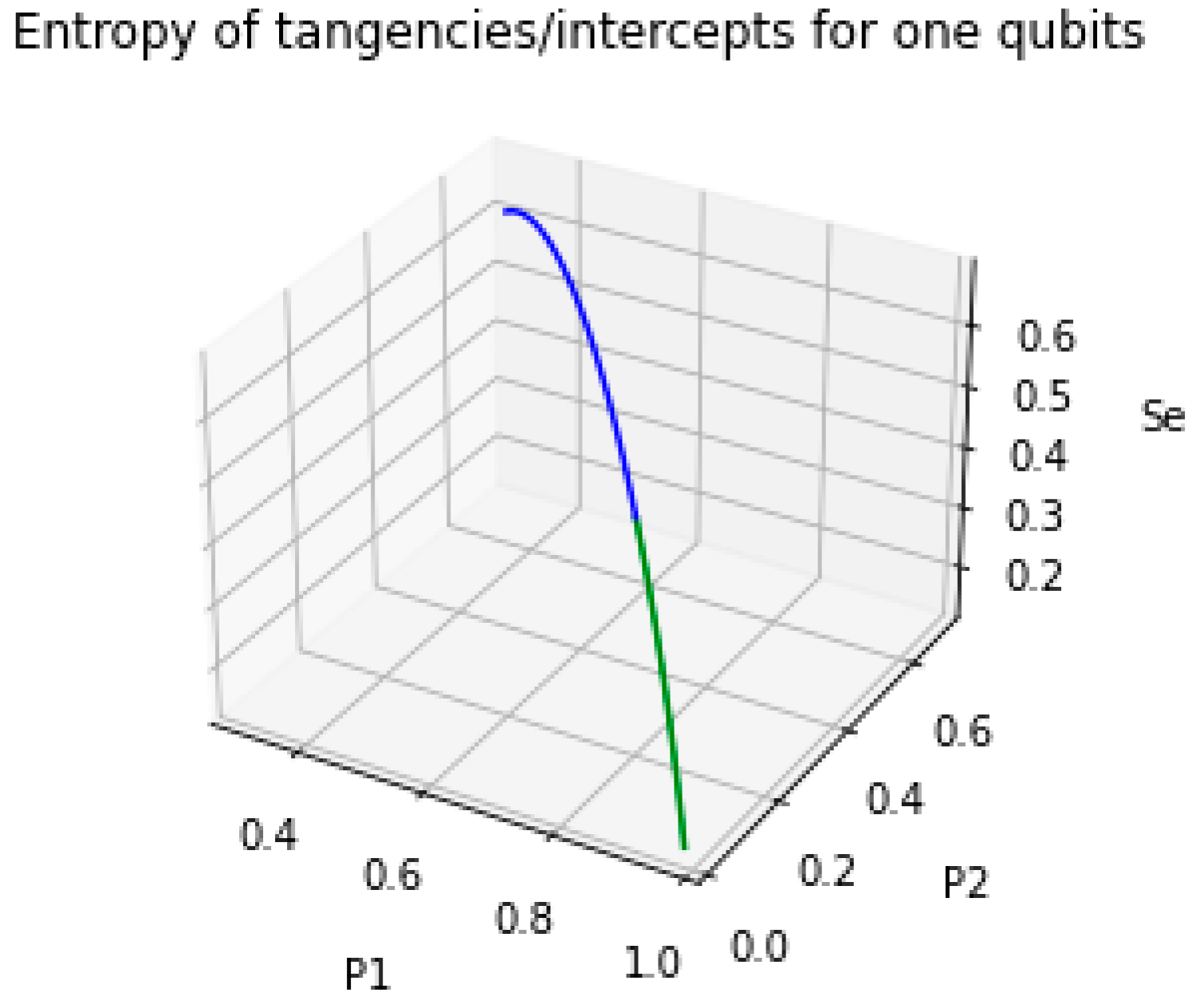
Entropy in the utility frameworkEntropy in quantum statesIn economics, entropy measures the various ways x and y can be organized to generate a certain level of utility. In quantum mechanics, entropy quantifies the uncertainty in the superposition of states. Both concepts reveal the complexity and constraints of the system.
Disclaimer/Publisher’s Note: The statements, opinions and data contained in all publications are solely those of the individual author(s) and contributor(s) and not of MDPI and/or the editor(s). MDPI and/or the editor(s) disclaim responsibility for any injury to people or property resulting from any ideas, methods, instructions or products referred to in the content.

