
A Potential-Based Quantization Procedure of the Damped Oscillator
1
Department of Physics, Budapest University of Technology and Economics, Budafoki út 8, H-1111 Budapest, Hungary
2
Department of Natural Sciences, Institute of Electrophysics, Kálmán Kandó Faculty of Electrical Engineering, Óbuda University, Tavaszmező u. 17, H-1084 Budapest, Hungary
3
Department of Natural Sciences, National University of Public Service, Ludovika tér 2, H-1083 Budapest, Hungary
*
Author to whom correspondence should be addressed.
Quantum Rep. 2022, 4(4), 390-400; https://doi.org/10.3390/quantum4040028
Submission received: 1 August 2022
/
Revised: 12 September 2022
/
Accepted: 16 September 2022
/
Published: 21 September 2022
Abstract
:Today, two of the most prosperous fields of physics are quantum computing and spintronics. In both, the loss of information and dissipation play a crucial role. In the present work, we formulate the quantization of the dissipative oscillator, which aids the understanding of the abovementioned issues, and creates a theoretical frame to overcome these issues in the future. Based on the Lagrangian framework of the damped spring system, the canonically conjugated pairs and the Hamiltonian of the system are obtained; then, the quantization procedure can be started and consistently applied. As a result, the damping quantum wave equation of the dissipative oscillator is deduced, and an exact damping wave solution of this equation is obtained. Consequently, we arrive at an irreversible quantum theory by which the quantum losses can be described.
1. Introduction
The existence of oscillator motion and the wave propagation mode are the necessary conditions for signal transmission, and consequently, information transfer. In a realistic quantum operation, the dissipation of a signal appears due to the loss of energy from a quantum system, for example, a single atom coupled to a single mode of electromagnetic radiation undergoes spontaneous emission [1]. This may happen in an ion trap quantum computation, as proposed by Cirac and Zoller [2]. Similarly, in spin-wave interconnects, spin-wave memories, or spin-wave transducers, and the attenuation reduces the efficiency, the lossy spin-wave propagation leads to fundamental limitations [3]. In the construction of quantum computers and further quantum information systems, the qubits are responsible for information transfer. A single electron on a solid neon surface provides the experimental realization of a new qubit platform [4]. In this realization, the limited coherent time is due to the energy and phase loss originating from the material surface deficiency and the noise of the environment.
These experiments and their theoretical discussions suggest the deeper understanding of dissipation of a single quantum package. The key to wave propagation is the oscillator; thus, it is worth dealing with the description of the quantized damped oscillator. The idea of quantizing the damped oscillator and the description of non-conserving energy subsystems coincide with the birth of quantum theory itself [5,6]. Based on their original idea of quantum dissipation, the description has been strongly developed [7]. In other research, the explicit time-dependent formulation can also provide a successful deduction of the dissipative oscillator [8,9]. However, the uncertainty principle is incompatible with the time-dependent mathematical structure [10]. The dissipative quantum systems can be modeled by the sets of decoupled harmonic oscillators in a reservoir [11,12,13]. The considered systems have a statistical behavior, so the observed dynamics differ from the motion of a single damped quantum oscillator.
Generally, the lack of success of the solution was due to several stumbling blocks in the construction. The first difficulty was immediately in the formulation of the Lagrangian; consequently, it was not possible to deduce the canonical variables, the Hamiltonian, and the Poission bracket expressions. Thus, the commutation rules, required for the quantization procedure, could not be formulated at all.
The problem of the missing Lagrangian structure of the dissipative systems was much older than the elaboration of the quantization procedure of conservative systems; it went back to Rayleigh [14]. The equation of motion (EOM) of the harmonic oscillator
is deduced from the Lagrangian of
where the related Euler–Lagrange equation is
To describe the damped oscillator, Rayleigh introduced the so-called dissipation potential—pertaining to the drag force —
by which the EOM could be recovered in the following way:
It is easy to check that the correct EOM appears:
However, it can be proven that the added term on the right side in Equation (5) is not from the least action principle, and the related variational calculus, i.e., the Lagrangian frame is lost. Much later Bateman [15] suggested a mirror image description in which a complementary equation appears due to the introduced function y. Here, the variation problem is
In addition to the damped oscillator equation, the mirror image equation is
While the equation of x relates to the damping solution, the equation of y pertains to an exponentially increasing amplitude motion. The calculated Hamiltonian includes both of these functions at the same time. It may cause a cumbersome explanation and elaboration of canonical variable pairs. A few years ago, Bagarello et al. proved that the canonical quantization for the damped harmonic oscillator using the Bateman Lagrangian did not work [16]. Similarly, Morse and Feshbach [17] used the variable duplication method for the diffusion problem. In this case, the diffusion variable was considered a complex quantity, and its complex conjugate pair was the duplicated variable. Here, interpretation was cumbersome, due to the complex diffusion functions and the related canonical formulation.
The application of the complex absorbing potentials—firstly used for the description of scattering processes [18,19,20,21,22,23,24,25,26]—may provide an opportunity for the description of dissipation and ireversibility in quantum theory. The method is that the Schrődinger equation is formulated by a complex potential , where represents the conservative potential, and pertains to the damping. Therefore, the EOM for this system is
The deduced balance equation for is
where just the complex part of the potential remains, generating the loss of the system. An obvious choice is to describe the motion of the quantum damped oscillator by the complex harmonic potential introduced by real-valued angular frequencies and [26]
The solution can be obtained by the application of the Feynman path integral method [27,28,29,30], as it was shown previously [26]. We see that this method stands on the complex generalization of the acting potential, and the dissipation appears as a consequence of this non-hermitian potential. However, we miss the direct—introduced by an “equation-level”—formulation of the dissipation.
An explicit time-dependent Lagrangian method using the WKB approximation in the quantization procedure was developed by Serhan et al. [31,32]. Despite the exponentially decreasing time-dependence of the wave function, it describes a standing solution in space.
A path integral method with a dynamical friction term was suggested for quantum dissipative systems by El-Nabulsi [33]. Here, Stokes’ drag force introduced the loss. However, the equation did not contain the velocity-dependent term. It contrasts with the standard EOM, which yields the usual exponential relaxation in time.
Presently, we apply the canonical quantization method for the damped harmonic oscillator. We point out this classically developed procedure works in dissipative cases not only with conservative potentials. We start from the EOM, and we formulate the Lagrangian and the Hamiltonian of the problem in general in Section 2. As a particular case, the Hamiltonian of the underdamped oscillator is expressed in Section 3. The canonical quantization procedure is described in Section 4, and the damping wave function is calculated by the path integral method in Section 5. The results are summarized in a short conclusion in Section 6.
The present technique has multiple advantages compared to the previous approaches. (i) The canonical expressions and the quantization steps are similar to the usual procedure. Thus, the developed description can be considered a generalization. (ii) The solving methods, such as the path integral method, can be applied without radical changes. (iii) The required necessary difference in the interpretation of the damped wave function can be interpreted.
2. The Lagrangian and Hamiltonian of a Damped Harmonic Oscillator
The quantization procedure requires the formulation of the complete Lagrangian–Hamiltonian frame first. To achieve this aim, we begin our examination with the EOM for the damped harmonic oscillator
where m is the mass, is a specific damping factor, and is the angular frequency. For the measurable quantity x, we define a generator potential q characterizing the underlying degrees of freedom, i.e., the definition equation can be obtained as in [34,35,36],
A suitable Lagrangian can be formulated by the potential
The equations of motion can be calculated from a Lagrangian of the general form
This method results in the EOM of the harmonic oscillator for the potential as the Euler–Lagrange equation. In general, Hamiltonian formalism requires canonical coordinate and momentum pairs
where . The Hamiltonian can be deduced from the abovementioned general Lagrangian as
For the present particular case, and , we obtain the relevant coordinates as
and
Moreover, the general expression for the momentum is
by which we calculate the particular case as
Similarly, we formulate the momentum
i.e.,
The Hamiltonian can be calculated by Equation (18). As a first step, we obtain it by the potential function q
The following step is to substitute the potential function with the coordinates and the momenta. We arrive at the canonical formulation of the Hamiltonian as
To preserve the energy-like unit of the Hamiltonian, we transform the coordinates and the momenta. The transformation means a simple product by , , and . Thus, we obtain new coordinates, and , and new momenta, and .
The meaning of the canonical moment and the canonical coordinate is the same as the mechanical momentum and the spatial coordinate. Moreover, the Hamiltonian, , is obtained
The units of the quantities are denoted by the bracket . Finally, the Hamiltonian of the damped oscillator is
Before we turn to the quantization procedure, it is worth examining a further property of this Hamiltonian. Since this Hamiltonian pertains to a dissipative process, we expect that this is a non-hermitian operator. The reason is that the probability does not conserve during dissipation. We will see later that the operators that belong to the first three terms are hermitian, but the fourth term is not. The fourth term operator will generate the dissipation in the description. Furthermore, the appearance of in the term similarly shows this fact.
3. The Devil Is in the Details
Since the formulation of the Lagrangian does not contain explicit time dependence, the Hamiltonian must be a constant value, i.e., the Hamiltonian expresses a conservation law. At this point, there is an open question of what the Hamiltonian exactly means. Here, we try to clarify the role of the Hamiltonian in this theory.
We focus just on the solutions that pertain to the underdamped and overdamped cases. As was shown previously by Szegleti et al. [34], the solution holds
where . The last two terms are proportional to the exponentially increasing , so they have non-physical meaning. Consequently, they could not have a role in the measurable . After the fit of the initial conditions for the measurable quantities, the position, and the velocity, and , keeping the physical solutions, the relevant potential is
Now, we are ready to substitute this generator’s potential function into the expression of the Hamiltonian in Equation (25). The mathematical calculation results in
and similarly,
by Equation (32). Since there is no explicit time dependence in the Lagrangian, the Hamiltonian must be constant. Generally, the Hamiltonian is the energy of the oscillating mass point. However, now the energy of the damped oscillator dissipates during the vibration. So, the non-zero energy cannot be the constant of motion. This strange result means that this zero value Hamiltonian is the conserved quantity of the damped oscillator. We may say there is no contradiction in the theory. However, the Hamiltonian loses the meaning of the “total energy of the system”. Despite this situation, we consider the Hamiltonian as an energy-like quantity. We will see that this zero value Hamiltonian in Equation (50) (see below) enables us to elaborate on the quantization formulation of the dissipative oscillator.
4. The Quantization Procedure
To achieve the state equation of the quantized damped oscillator, we need to identify the canonical momenta in the Hamiltonian, , in Equation (32). In the case of the canonical pair from Equations (27) and (28), we introduce into the transformed space the spatial coordinate y
The momentum and the coordinate are the usual canonically conjugated pairs. The construction of the momentum and the coordinate are based on Equations (29) and (30) and a comparison with the momentum and the coordinate in Equation (37). The appearing time factor in Equations (29) and (30) can be associated with Fourier transformed pairs, i.e.,
The terms of the Hamiltonian can be expressed in the operator formulation applying the above rules. The calculation of and proceeds as is usual.
Applying the above Fourier formulations, we can obtain the commutation rules
We take from Equation (37) and the first Fourier transform in Equation (39); then, we obtain
The second term includes the product. Now, we consider from Equation (37) and from Equation (38); then, we apply the third Fourier transform in Equation (39). The detailed steps are shown one by one
by which we obtain the second term of the Hamiltonian in the operator formalism
We continue with the term. We take from Equation (38) and from Equation (37), and we apply the second and fourth Fourier transform, i.e.,
The last term of the Hamiltonian includes the product. The relevant substitutions come from Equation (37), and we consider the fourth Fourier transform
by which we write
Taking the Hamiltonian in Equation (32), the fact that in Equation (36), and substituting these expressions into it, the quantized state equation of the damped oscillator can be formulated as
Now, we can recognize the importance of the zero-valued Hamiltonian. Similar to the complex absorbing potential in Equation (11), a non-hermitian term appears in the state equation. Its role is the same as the term that generates dissipation in the motion. However, the deduction of the damped state equation comes from a consequent calculation; the complex part of the potential in Equation (11) is an ad hoc assumption. We can divide the equation into the undamped quantum harmonic oscillator and the damping part. The damping term also includes the quantum action factor ℏ.
5. Solution of Damping Wave Equation
The oscillation starts from a normalized Gaussian shape initial wave function, which is the eigenfunction of the lowest-lying energy level of the frictionless case:
with its center position . The movement of the undamped oscillator (the frictionless part of Equation (50)) can be calculated by the Feynman path integral method [27,28,29,30]. Souriau pointed out a correction that is necessary beyond the first half-period of motion in the integration formula of Feynman [39]. However, a further detailed study was to refine the oscillator wave packet motion. Naqvi and Waldenstrøm [40] introduced a parameter by which the width of the Gaussian wave packet changes periodically in time around the origin (see Figure 2 in Ref. [26])
where
ensures the width change.
The first two terms in Equation (50) do not depend on the time, and since the third term includes a first-order time derivative, the damping effect can be extracted from the third and fourth terms (see Appendix A), i.e.,
The solution to this equation can be expressed as
Finally, we obtain the exact solution of the quantum dissipative oscillator Equation (50) as
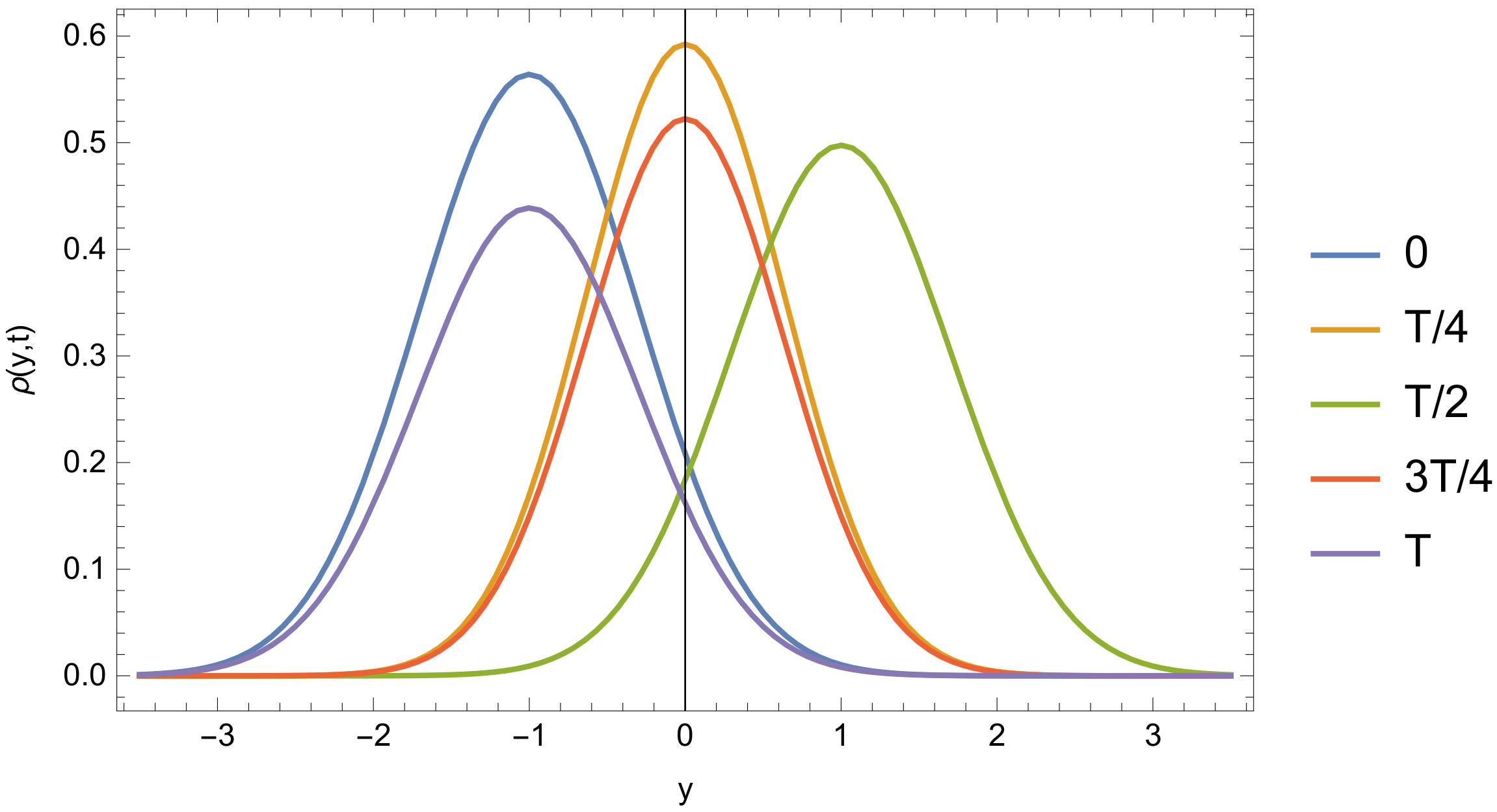
The time evolution of is presented in Figure 1, as it is similarly experienced from the complex potential approximations in the description of dissipative quantum systems [18,26]. However, in the present quantization procedure, the damped oscillator frequency is identical to the frequency of the undamped oscillator. In contrast to the classic case, the damping does not modify the eigenfrequency , i.e., the damping pertains to the energy and information loss. This fact suggests that the well-known Lorentz distribution in the scattering process does not relate to a frequency shift due to the damping effect on a quantum level. On the other hand, this result is in line with the second quantized solution in Ref. [41]. In this reference, Equation (A4.21) clearly shows that there is no frequency shift in the case of a damped quantum oscillator but just amplitude damping. The experimental and theoretical motivations for the quantum dissipation can be found in the early Refs. [42,43].
A time series of with parameters set as , , , and is shown in Figure 1 in which the evolution can be easily followed in one time period.
The damping of the quantum dissipative oscillator arises from the smooth function , so the graph is similar for higher values.
6. Conclusions
We presented a thorough investigation and a solution for the age-old problem, the quantization of the damped oscillator. The information loss is closely related to the signal distortion, i.e., the energy dissipation. Our method overcame the limitations of the previous formulations using several means to achieve the damping state equation. We returned to the fundamentals of quantum theory, such as (i) the Lagrangian formulation, (ii) the Hamiltonian canonical description, and (iii) the quantization procedure. Thus, we applied this mathematical framework to the damping oscillator. In possession of the correct Lagrangian description, the way opened toward the quantization procedure. As was shown, a remarkably understandable damping state equation energed. Finally, we calculated the exact solution of this quantum dissipative oscillator equation. We conclude that a consequent construction of the damping quantum oscillator equation is presented by the exact solution of this damped state equation. However, we emphasize that due to the non-hermitian complex potential, the probability meaning of the wave function is lost. The results bring us closer to the understanding of energy dissipation, information loss, and the maximal probability of the recovery of a signal on the microscopic level. Our studies in the area of quantum dissipation require further discussion and examination.
Author Contributions
The authors contributed equally to this work. All authors have read and agreed to the published version of the manuscript.
Funding
This research was supported by the National Research, Development and Innovation Office (NKFIH), Grant Nr. K137852, and by the Ministry of Innovation and Technology and the NKFIH within the Quantum Information National Laboratory of Hungary. Project no. TKP2021-NVA-16 was implemented with the support provided by the Ministry of Innovation and Technology of Hungary from the National Research, Development and Innovation Fund.
Data Availability Statement
Not applicable.
Conflicts of Interest
The authors declare no conflict of interest.
Appendix A
We point out that the solution of the damping quantum oscillator equation can be exactly obtained as a product of the solution of the undamped oscillator and an exponentially decreasing time-dependent function. We start from the dissipative state equation by repeating Equation (50)
Let us denote the solution of the undamped oscillator by
i.e.,
is completed. Now, we find the solution to the damped equation in the form
It is easy to check by substitution that this function is a solution to the problem:
Since the last two terms eliminate each other, we retain the undamped part of the problem. However, we assume that is the solution to the undamped motion. Q.E.D.
References
- Nielsen, M.A.; Chuang, I.L. Quantum Computation and Quantum Information; Cambridge Universdity Press: Cambridge, UK, 2010. [Google Scholar]
- Cirac, J.I.; Zoller, P. Quantum Computations with Cold Trapped Ions. Phys. Rev. Lett. 1995, 74, 4091. [Google Scholar] [CrossRef]
- Mahmoud, A.; Ciubotaru, F.; Vanderveken, F.; Chumak, A.V.; Hamdioui, S.; Adelmann, C.; Cotofana, S. Introduction to Spin Wave Computing. J. Appl. Phys. 2020, 128, 161101. [Google Scholar] [CrossRef]
- Zhou, X.; Koolstra, G.; Zhang, X.; Yang, G.; Han, X.; Dizdar, B.; Li, X.; Divan, R.; Guo, W.; Murch, K.W.; et al. Single electrons on solid neon as a solid-state qubit platform. Nature 2022, 605, 46. [Google Scholar] [CrossRef] [PubMed]
- Caldirola, P. Forze non conservative nella meccanica quantistica. Il Nuovo C. 1941, 18, 393. [Google Scholar] [CrossRef]
- Kanai, E. On the Quantization of the Dissipative Systems. Prog. Theor. Phys. 1948, 3, 440. [Google Scholar] [CrossRef]
- Choi, J.R. Analysis of Quantum Energy for Caldirola–Kanai Hamiltonian Systems in Coherent States. Results in Phys. 2013, 3, 115. [Google Scholar] [CrossRef]
- Dekker, H. Classical and Quantum Mechanics of the Damped Harmonic Oscillator. Phys. Rep. 1981, 80, 1. [Google Scholar] [CrossRef]
- Dittrich, W.; Reuter, M. Classical and Quantum Dynamics; Springer: Berlin/Heidelberg, Germany, 1996. [Google Scholar]
- Weiss, U. Quantum Dissipative Systems; World Scientific: Singapore, 2012. [Google Scholar]
- Leggett, A.J. Quantum Tunneling in the Presence of an Arbitrary Linear Dissipation Mechanism. Phys. Rev. B 1984, 30, 1208. [Google Scholar] [CrossRef]
- Caldeira, A.O.; Neto, A.H.C.; de Carvalho, T.O. Dissipative Quantum Systems Modeled by a Two-level-reservoir Coupling. Phys. Rev. B 1993, 48, 13974. [Google Scholar] [CrossRef]
- Da Costa, M.R.; Caldeira, A.O.; Dutra, S.M.; Westfahl, H. Exact Diagonalization of Two Quantum Models for the Damped Harmonic Oscillator. Phys. Rev. A 2000, 61, 022107. [Google Scholar] [CrossRef] [Green Version]
- Rayleigh, J.W.S. The Theory of Sound; Dover: New York, NY, USA, 1929. [Google Scholar]
- Bateman, H. On Dissipative Systems and Related Variational Principles. Phys. Rev. 1931, 38, 815. [Google Scholar] [CrossRef]
- Bagarello, F.; Gargano, F.; Roccati, F. A No-go Result for the Quantum Damped Harmonic Oscillator. Phys. Lett. A 2019, 383, 2836. [Google Scholar] [CrossRef]
- Morse, P.M.; Feshbach, H. Methods of Theoretical Physics; McGraw-Hill: New York, NY, USA, 1953. [Google Scholar]
- Razavy, M. Classical and Quantum Dissipative Systems; Imperial College Press: London, UK, 2005; p. 129. [Google Scholar]
- Vibók, Á.; Balint-Kurti, G.G. Reflection and Transmission of Waves by a Complex Potential—A Semiclassical Jeffreys–Wentzel– Kramers–Brillouin Treatment. J. Chem. Phys. 1992, 96, 7615. [Google Scholar] [CrossRef]
- Vibók, Á.; Balint-Kurti, G.G. Parametrlzatlon of Complex Absorbing Potentials for Time-Dependent Quantum Dynamics. J. Chem. Phys. 1992, 96, 8712. [Google Scholar] [CrossRef]
- Halász, G.J.; Vibók, Á. Using a Multi-step Potential as an Exact Solution of the Absorbing Potential Problem on the Grid. Chem. Phys. Lett. 2000, 323, 287. [Google Scholar] [CrossRef]
- Vibók, Á.; Halász, G.J. Parametrization of Complex Absorbing Potentials for Time-dependent Quantum Dynamics Using Multi-step Potentials. Phys. Chem. Chem. Phys. 2001, 3, 3048. [Google Scholar] [CrossRef]
- Halász, G.J.; Vibók, Á. Comparison of the Imaginary and Complex Absorbing Potentials Using Multistep Potential Method. Int. J. Quantum Chem. 2003, 92, 168. [Google Scholar] [CrossRef]
- Muga, J.G.; Palao, J.P.; Navarro, B.; Egusquiza, I.L. Complex Absorbing Potentials. Phys. Rep. 2004, 395, 357. [Google Scholar] [CrossRef]
- Henderson, T.M.; Fagas, G.; Hyde, E.; Greer, J.C. Determination of Complex Absorbing Potentials from the Electron Self-energy. J. Chem. Phys. 2006, 125, 244104. [Google Scholar] [CrossRef]
- Márkus, B.G.; Márkus, F. Quantum Particle Motion in Absorbing Harmonic Trap. Indian J. Phys. 2016, 90, 441. [Google Scholar] [CrossRef] [Green Version]
- Feynman, R.P.; Hibbs, A.R. Quantum Mechanics and Path Integrals; McGraw-Hill: New-York, NY, USA, 1965. [Google Scholar]
- Feynman, R.P. Statistical Mechanics; Addison-Wesley: Reading, MA, USA, 1994. [Google Scholar]
- Khandekar, D.C.; Lawande, S.V. Feynman Path Integrals: Some Exact Results and Applications. Phys. Rep. 1986, 137, 115. [Google Scholar] [CrossRef]
- Dittrich, W.; Reuter, M. Classical and Quantum Dynamics; Springer: Berlin/Heidelberg, Germany, 1992; pp. 179–208. [Google Scholar]
- Serhan, M.; Abusini, M.; Al-Jamel, A.; El-Nasser, H.; Rabei, E.M. Quantization of the Damped Harmonic Oscillator. J. Math. Phys. 2018, 59, 082105. [Google Scholar] [CrossRef]
- Serhan, M.; Abusini, M.; Al-Jamel, A.; El-Nasser, H.; Rabei, E.M. Response to Comment on ‘Quantization of the Damped Harmonic Oscillator’. J. Math. Phys. 2019, 60, 094101. [Google Scholar] [CrossRef]
- El-Nabulsi, R.A. Path Integral Method for Quantum Dissipative Systems with Dynamical Friction: Applications to Quantum Dots/Zero-dimensional Nanocrystals. Superlattices Microstruct 2020, 144, 106581. [Google Scholar] [CrossRef]
- Szegleti, A.; Márkus, F. Dissipation in Lagrangian Formalism. Entropy 2020, 29, 930. [Google Scholar] [CrossRef] [PubMed]
- Gambár, K.; Márkus, F. Hamilton-Lagrange Formalism of Nonequilibrium Thermodynamics. Phys. Rev. E 1994, 50, 1227. [Google Scholar] [CrossRef] [PubMed]
- Gambár, K.; Rocca, M.C.; Márkus, F. A Repulsive Interaction in Classical Electrodynamics. Acta Polytechn. Hung. 2020, 17, 175. [Google Scholar] [CrossRef]
- Ostrogradski, M. Mémoires sur les équations différentielles, relatives au problème des isopérimètres. Mem. Ac. St. Petersbourg 1850, 6, 385. [Google Scholar]
- Courant, R.; Hilbert, D. Methods of Mathematical Physics; Interscience: New York, NY, USA, 1966. [Google Scholar]
- Souriau, J.M. Construction Explicite de l’indice de Maslov. Applications, in “Group Theoretical Methods in Physics”; Fourth Internat. Colloq.: Nijmegen, The Netherlands, 1975; pp. 117–148. [Google Scholar]
- Naqvi, K.R.; Waldenstrøm, S. Revival, Mirror Revival and Collapse may Occur even in a Harmonic Oscillator Wave Packet. Phys. Scr. 2000, 62, 12. [Google Scholar] [CrossRef]
- Risken, H. The Fokker-Planck Equation: Methods of Solution and Applications, 2nd ed.; Springer: Berlin/Heidelberg, Germany, 1989; Appendix A.4; pp. 425–428. [Google Scholar]
- Haken, H. Laser Theory, Encyclopedia of Physics; Springer: Berlin/Heidelberg, Germany; New York, NY, USA, 1970; Volume XXV/2c. [Google Scholar]
- Haake, F. Springer Tracts Modern Physics; Springer: Berlin/Heidelberg, Germany; New York, NY, USA, 1973; Volume 66, pp. 98–168. [Google Scholar]
Figure 1.
The dissipation caused shape damping of the distribution of the damped oscillator in one time period. The applied parameter set is ; ; , , . The time period is . The peak of the initial distribution is at .
Figure 1.
The dissipation caused shape damping of the distribution of the damped oscillator in one time period. The applied parameter set is ; ; , , . The time period is . The peak of the initial distribution is at .
Publisher’s Note: MDPI stays neutral with regard to jurisdictional claims in published maps and institutional affiliations. |
© 2022 by the authors. Licensee MDPI, Basel, Switzerland. This article is an open access article distributed under the terms and conditions of the Creative Commons Attribution (CC BY) license (https://creativecommons.org/licenses/by/4.0/).
Share and Cite
MDPI and ACS Style
Márkus, F.; Gambár, K. A Potential-Based Quantization Procedure of the Damped Oscillator. Quantum Rep. 2022, 4, 390-400. https://doi.org/10.3390/quantum4040028
AMA Style
Márkus F, Gambár K. A Potential-Based Quantization Procedure of the Damped Oscillator. Quantum Reports. 2022; 4(4):390-400. https://doi.org/10.3390/quantum4040028
Chicago/Turabian StyleMárkus, Ferenc, and Katalin Gambár. 2022. "A Potential-Based Quantization Procedure of the Damped Oscillator" Quantum Reports 4, no. 4: 390-400. https://doi.org/10.3390/quantum4040028