Information Geometric Perspective on Off-Resonance Effects in Driven Two-Level Quantum Systems

Abstract

We present an information geometric analysis of off-resonance effects on classes of exactly solvable generalized semi-classical Rabi systems. Specifically, we consider population transfer performed by four distinct off-resonant driving schemes specified by $\mathrm{su}\left(2;ℂ\right)$ time-dependent Hamiltonian models. For each scheme, we study the consequences of a departure from the on-resonance condition in terms of both geodesic paths and geodesic speeds on the corresponding manifold of transition probability vectors. In particular, we analyze the robustness of each driving scheme against off-resonance effects. Moreover, we report on a possible tradeoff between speed and robustness in the driving schemes being investigated. Finally, we discuss the emergence of a different relative ranking in terms of performance among the various driving schemes when transitioning from on-resonant to off-resonant scenarios.

1. Introduction

It is well-known that the resonance phenomenon concerns the amplification that occurs when the frequency of an externally applied field (for instance, a magnetic field) is equal to a natural characteristic frequency of the system on which it acts. When a field is applied at the resonant frequency of another system, the system oscillates at a higher amplitude than when the field is applied at a non-resonant frequency. In an actual experimental laboratory, off-resonance effects can occur for a number of reasons. For instance, a common source of off-resonance effects is the presence of unforeseen magnetic field gradients that are not part of the externally applied magnetic field. These gradients can cause signal loss and, as a consequence, signals at the “wrong” resonant frequency (that is, off-resonance). Furthermore, when the intensity of an applied magnetic field gradient is changed in a laboratory, decaying eddy currents can produce time-varying off-resonant effects [1]. Additionally, the presence of concomitant gradients can create off-resonance effects in the form of $xy$-spatial variations in the Larmor frequency when a magnetic field gradient in the z-direction is applied [2]. For the interested reader, we discuss two illustrative examples concerning the departure from the on-resonance condition in the context of classical and quantum mechanics in Appendix A.

The resonance phenomenon happens to play a key role in problems where one seeks to drive an initial source state towards a final target state. For instance, typical problems of this kind can be found when controlling population transfer in quantum systems [3,4,5] or when searching for a target state [6,7]. In the framework of quantum control theory, it is commonly believed that an off-resonant driving scheme cannot help achieving population transfer with high fidelity between two quantum states. However, there do exist theoretical investigations relying on the phenomenon of superoscillations [8] where population transfer occurs by using only off-resonant driving fields [9]. In particular, during resonant superoscillations, the quantum system is temporarily excited and behaves as if truly driven at resonance [9]. Furthermore, the existence of suboptimal transfer efficiencies, caused by the sequential use of two lasers in order to physically realize a transition from highly excited Rydberg states to ground states [10,11], leads to question the possibility of transition from a ground state to the Rydberg state by means of lasers far-off-resonant with respect to the transition frequency. Indeed, motivated by such possibility, driving schemes specified by periodic square-wells and Gaussian pulses in order to implement coherent transfer with far-off-resonant driving fields have been proposed in reference [12].

It is also well-known that on-resonance driving is not a good control strategy for a quantum system if, from an experimental standpoint, one allows the Rabi frequency (that is, the frequency that describes the coupling between the driving field and the two-level system) to be higher than the Larmor frequency (that is, the characteristic transition frequency of the two-level system in the absence of the external driving field) [13]. This is called the strong driving regime. In such a scenario, the so-called rotating wave approximation (RWA, [14]) is not applicable and the system is driven with an external field whose amplitude is greater than or equal to the energy splitting between the system’s states. For an analysis on the deviation from sinusoidal Rabi oscillations by studying the time-evolution dynamics of a strongly driven dressed electron spin in silicon, we refer to reference [15]. Furthermore, for an explicit manifestation of strong sensitivity to the initial phase of the driving field in the dynamics of a general semi-classical Rabi model in regimes of arbitrary strong driving, we refer to reference [16].

Based upon our considerations, it is clear that off-resonance phenomena exhibit both experimental (for instance, limited control of spurious electromagnetic signals and strong driving regimes) and theoretical (for instance, sensitivity to initial conditions and emergence of more complex dynamical scenarios) interest. In the framework of analog quantum searching, we have recently presented a detailed investigation concerning the physical connection between quantum search Hamiltonians and exactly solvable time-dependent two-level quantum systems in reference [7]. In references [17,18], instead, we analyzed the possibility of modifying the original Farhi-Gutmann Hamiltonian quantum search algorithm [19] in order to speed up the procedure for producing a suitably distributed unknown normalized quantum mechanical state provided only a nearly optimal fidelity is sought. In reference [20], we presented an information geometric characterization of the oscillatory or monotonic behavior of statistically parametrized squared probability amplitudes originating from special functional forms of the Fisher information function: constant, exponential decay, and power-law decay. Furthermore, for each case, we computed both the computational speed and the availability loss of the corresponding physical processes by exploiting a convenient Riemannian geometrization of useful thermodynamical concepts. Finally, building upon our works presented in references [7,17,18,20], we presented in reference [21] an information geometric analysis of geodesic speeds and entropy production rates in geodesic motion on manifolds of parametrized quantum states. These pure states emerged as outputs of suitable $\mathrm{su}\left(2;ℂ\right)$ time-dependent Hamiltonian evolutions used to describe distinct types of analog quantum search schemes viewed as driving strategies. In particular, by evaluating the geodesic speed and the total entropy production along the optimum transfer paths in a number of physical scenarios of interest in analog quantum search problems (for instance, constant, oscillatory, power-law decay, and exponential decay of the driving magnetic fields), we showed in an explicit quantitative manner that to a faster transfer there corresponds necessarily a higher entropy production rate. Thus, we concluded that lower entropic efficiency values do appear to accompany higher entropic geodesic speed values in quantum transfer processes. Our information geometric analysis in reference [21] was limited to the case in which the on-resonance driving condition was satisfied for all quantum driving strategies. However, based upon our previous considerations, it would be of theoretical interest to investigate from an information geometric perspective the effects of off-resonance effects on these driving strategies. In particular, we would like to address the following questions:

(i)

What are the main effects of deviations from the on-resonance condition in these $\mathrm{su}\left(2;ℂ\right)$ time-dependent Hamiltonian evolutions?

(ii)

Do off-resonance effects modify (with respect to the on-resonance scenario) the relative ranking in terms of performance (quantified in terms of geodesic speed and/or minimum transfer time) among the driving schemes being considered?

(iii)

Are there driving schemes that are especially robust against deviations from the on-resonance condition and that, in addition, are capable of reaching sufficiently high fidelity values?

The rest of the paper is organized as follows. In Section 2, we present our driving strategies in terms of classes of exactly solvable generalized semi-classical Rabi systems. Specifically, we consider the population transfer performed by four distinct off-resonant driving schemes specified by $\mathrm{su}\left(2;ℂ\right)$ time-dependent Hamiltonian models. In Section 3, we propose our information geometric analysis of off-resonance effects on such classes of systems. For each scheme, we study the consequences of a departure from the on-resonance condition in terms of both geodesic paths and geodesic speeds on the corresponding manifold of transition probability vectors. In particular, we analyze the robustness of each driving scheme against off-resonance effects. Moreover, we report on a possible tradeoff between speed and robustness in the driving schemes being investigated. Finally, we discuss the emergence of a different relative ranking in terms of performance among the various driving schemes when transitioning from the on-resonant to the off-resonant scenarios. Our conclusive remarks appear in Section 4. Auxiliary illustrative examples together with some technical details are placed in Appendices Appendix A and Appendix B.

2. The su$(2$; $ℂ)$ Quantum Driving

In this section, we introduce our driving strategies in terms of classes of exactly solvable generalized semi-classical Rabi systems [22,23].

The quantum evolution we take into consideration is specified by means of an Hamiltonian operator ${\mathcal{H}}_{\mathrm{su}\left(2;ℂ\right)}$ written as the most general linear superposition of the three traceless and anti-Hermitian generators $\left\{i{\sigma }_x,-i{\sigma }_y,i{\sigma }_z\right\}$ of $\mathrm{su}\left(2;ℂ\right)$, the Lie algebra of the special unitary group $\mathrm{SU}\left(2;ℂ\right)$,

$${\mathcal{H}}_{\mathrm{su}\left(2;ℂ\right)}\left(t\right)\stackrel{\mathrm{def}}{=}a\left(t\right)\left(i{\sigma }_x\right)+b\left(t\right)\left(-i{\sigma }_y\right)+c\left(t\right)\left(i{\sigma }_z\right).$$

(1)

In Equation (1), $a\left(t\right)$, $b\left(t\right)$, and $c\left(t\right)$ are time-dependent complex coefficients while $\overrightarrow{\sigma }\stackrel{\mathrm{def}}{=}\left({\sigma }_x,{\sigma }_y,{\sigma }_z\right)$ denotes the Pauli vector operator. In particular, by putting $a\left(t\right)\stackrel{\mathrm{def}}{=}-i{\omega }_x\left(t\right)$, $b\left(t\right)\stackrel{\mathrm{def}}{=}i{\omega }_y\left(t\right)$, and $c\left(t\right)\stackrel{\mathrm{def}}{=}-i\Omega \left(t\right)$, Equation (1) yields

$${\mathcal{H}}_{\mathrm{su}\left(2;ℂ\right)}\left(t\right)\stackrel{\mathrm{def}}{=}{\omega }_x\left(t\right){\sigma }_x+{\omega }_y\left(t\right){\sigma }_y+\Omega \left(t\right){\sigma }_z.$$

(2)

In the framework of $\mathrm{su}\left(2;ℂ\right)$ Hamiltonian models, $\omega \left(t\right)\stackrel{\mathrm{def}}{=}{\omega }_x\left(t\right)-i{\omega }_y\left(t\right)={\omega }_{\mathcal{H}}\left(t\right)e^{i{\varphi }_{\omega }\left(t\right)}$ and $\Omega \left(t\right)$ are the so-called complex transverse field and real longitudinal field, respectively. Obviously, ${\omega }_{\mathcal{H}}\left(t\right)$ denotes the modulus of $\omega \left(t\right)$. In what follows, we assume that longitudinal fields $\Omega \left(t\right)$ are oriented along the z-axis while transverse fields $\omega \left(t\right)$ lie in the $xy$-plane. Taking into consideration the quantum evolution of an electron (or, more generally, a spin-$1/2$ particle) in an external time-dependent magnetic field $\overrightarrow{B}\left(t\right)$, the Hamiltonian ${\mathcal{H}}_{\mathrm{su}\left(2;ℂ\right)}\left(t\right)$ in Equation (2) can be rewritten as

$${\mathcal{H}}_{\mathrm{su}\left(2;ℂ\right)}\left(t\right)\stackrel{\mathrm{def}}{=}-\overrightarrow{\mu }·\overrightarrow{B}\left(t\right),$$

(3)

where $\overrightarrow{\mu }\stackrel{\mathrm{def}}{=}\left(eħ/2mc\right)\overrightarrow{\sigma }$ denotes the magnetic moment of the electron with ${\mu }_{\mathrm{Bohr}}\stackrel{\mathrm{def}}{=}\left|e\right|ħ/\left(2mc\right)\simeq 9.27\times {10}^{-21}\left[\mathrm{cgs}\right]$ being the so-called Bohr magneton. The quantity $m\simeq 9.11\times {10}^{-31}\left[\mathrm{MKSA}\right]$ is the mass of an electron while $\left|e\right|\simeq 1.60\times {10}^{-19}\left[\mathrm{MKSA}\right]$ denotes the absolute value of the electric charge of an electron. Moreover, $c\simeq 3\times {10}^8\left[\mathrm{MKSA}\right]$ and $ħ\simeq 1.05\times {10}^{-34}\left[\mathrm{MKSA}\right]$ are the speed of light and the reduced Planck constant, respectively. The magnetic field $\overrightarrow{B}\left(t\right)$ in Equation (1) can be recast as

$$\overrightarrow{B}\left(t\right)\stackrel{\mathrm{def}}{=}{\overrightarrow{B}}_{\perp }\left(t\right)+{\overrightarrow{B}}_{\Vert }\left(t\right),$$

(4)

with ${\overrightarrow{B}}_{\perp }\left(t\right)\stackrel{\mathrm{def}}{=}{B}_x\left(t\right)\widehat{x}+B_y\left(t\right)\widehat{y}$ and ${\overrightarrow{B}}_{\Vert }\left(t\right)\stackrel{\mathrm{def}}{=}{B}_z\left(t\right)\widehat{z}$. Equating the Hamiltonians in Equations (2) and (3) and making use of the magnetic field decomposition in Equation (4), the connection between the set of field intensities $\left\{{\omega }_{\mathcal{H}}\left(t\right),{\Omega }_{\mathcal{H}}\left(t\right)\right\}$ and the set of magnetic field intensities $\left\{B_{\perp }\left(t\right),B_{\Vert }\left(t\right)\right\}$ becomes clear. More specifically, we observe that $B_{\perp }\left(t\right)\propto {\omega }_{\mathcal{H}}\left(t\right)$ and $B_{\Vert }\left(t\right)\propto$${\Omega }_{\mathcal{H}}\left(t\right)\stackrel{\mathrm{def}}{=}\left|\Omega \left(t\right)\right|$. The exact connection between the components $\left\{B_x\left(t\right),B_y\left(t\right),B_z\left(t\right)\right\}$ and $\left\{{\omega }_x\left(t\right),{\omega }_y\left(t\right),\Omega \left(t\right)\right\}$ is expressed by

$$B_x\left(t\right)=-\frac{2mc}{eħ}{\omega }_x\left(t\right),B_y\left(t\right)=-\frac{2mc}{eħ}{\omega }_y\left(t\right),\mathrm{and}{B}_z\left(t\right)=-\frac{2mc}{eħ}\Omega \left(t\right).$$

(5)

Moreover, in terms of field intensities, we get

$$B_{\perp }\left(t\right)=\frac{2mc}{\left|e\right|ħ}{\omega }_{\mathcal{H}}\left(t\right),\mathrm{and}{B}_{\Vert }\left(t\right)=\frac{2mc}{\left|e\right|ħ}{\Omega }_{\mathcal{H}}\left(t\right).$$

(6)

Studying the quantum evolution of an electron governed by the Hamiltonian in Equation (3) by means of exact analytical expressions of complex probability amplitudes and/or real transition probabilities from an initial source state to a final target state can be quite challenging. In particular, the canonical matrix representations of ${\mathcal{H}}_{\mathrm{su}\left(2;ℂ\right)}$ in Equation (2) and $\mathcal{U}\left(t\right)$, the unitary evolution operator arising from ${\mathcal{H}}_{\mathrm{su}\left(2;ℂ\right)}$, with $iħ\dot{\mathcal{U}}\left(t\right)={\mathcal{H}}_{\mathrm{su}\left(2;ℂ\right)}\mathcal{U}\left(t\right)$ and $\dot{\mathcal{U}}\stackrel{\mathrm{def}}{=}{\partial }_t\mathcal{U}$, are given by

$$\left[{\mathcal{H}}_{\mathrm{su}\left(2;ℂ\right)}\right]\stackrel{\mathrm{def}}{=}\left(\begin{array}{cc}\Omega \left(t\right)& \omega \left(t\right)\\ {\omega }^{*}\left(t\right)& -\Omega \left(t\right)\end{array}\right),\mathrm{and}\left[\mathcal{U}\left(t\right)\right]\stackrel{\mathrm{def}}{=}\left(\begin{array}{cc}\alpha \left(t\right)& \beta \left(t\right)\\ -{\beta }^{*}\left(t\right)& {\alpha }^{*}\left(t\right)\end{array}\right),$$

(7)

respectively. The unitarity of the quantum evolution demands that the complex probability amplitudes $\alpha \left(t\right)$ and $\beta \left(t\right)$ fulfill the normalization condition, ${\left|\alpha \left(t\right)\right|}^2+{\left|\beta \left(t\right)\right|}^2=1$. Once the unitary evolution operator $\mathcal{U}\left(t\right)$ in Equation (7) is given, the temporal evolution of a quantum source state $\left|s\right.〉$,

$$\left|s\right.〉\stackrel{\mathrm{def}}{=}x\left|w\right.〉+\sqrt{1-x^2}\left|w_{\perp }\right.〉,$$

(8)

can be characterized by the following transformation law,

$$\left(\genfrac{}{}{0pt}{}{x}{\sqrt{1-x^2}}\right)\to \left(\genfrac{}{}{0pt}{}{\alpha \left(t\right)x+\beta \left(t\right)\sqrt{1-x^2}}{-{\beta }^{*}\left(t\right)x+{\alpha }^{*}\left(t\right)\sqrt{1-x^2}}\right),$$

(9)

with $x\stackrel{\mathrm{def}}{=}〈w|s〉$ denoting the quantum overlap. The set of orthonormal state vectors $\left\{\left|w\right.〉,\left|w_{\perp }\right.〉\right\}$ generate the two-dimensional search space of the $N=2^n$-dimensional complex Hilbert space ${\mathcal{H}}_2^n$. Therefore, using Equations (7), (8), and (9), the probability that the source state $\left|s\right.〉$ transitions into the target state $\left|w\right.〉$ under $\mathcal{U}\left(t\right)$ becomes

$${\mathcal{P}}_{\left|s\right.〉\to \left|w\right.〉}\left(t\right)\stackrel{\mathrm{def}}{=}{\left|〈w|\mathcal{U}\left(t\right)|s〉\right|}^2={\left|\alpha \left(t\right)\right|}^2{x}^2+{\left|\beta \left(t\right)\right|}^2\left(1-x^2\right)+\left[\alpha \left(t\right){\beta }^{*}\left(t\right)+{\alpha }^{*}\left(t\right)\beta \left(t\right)\right]x\sqrt{1-x^2}.$$

(10)

It is evident from Equation (10) that in order to calculate the exact analytical expression of transition probabilities, one must have the exact analytical formula of the evolution operator $\mathcal{U}\left(t\right)$ expressed in terms of the complex probability amplitudes $\alpha \left(t\right)$ and $\beta \left(t\right)$. Ideally, having specified the fields $\omega \left(t\right)$ and $\Omega \left(t\right)$ by means of physical arguments, one would solve the coupled system of first order ordinary differential equations with time-dependent coefficients emerging from the relation $iħ\dot{\mathcal{U}}\left(t\right)={\mathcal{H}}_{\mathrm{su}\left(2;ℂ\right)}\mathcal{U}\left(t\right)$ with $\mathcal{U}\left(0\right)=\mathcal{I}$,

$$iħ\dot{\alpha }\left(t\right)=\Omega \left(t\right)\alpha \left(t\right)-\omega \left(t\right){\beta }^{*}\left(t\right),\mathrm{and}iħ\dot{\beta }\left(t\right)=\omega \left(t\right){\alpha }^{*}\left(t\right)+\Omega \left(t\right)\beta \left(t\right),$$

(11)

where $\alpha \left(0\right)=1$ and $\beta \left(0\right)=0$. However, it is often the case that this general approach does not yield exact analytical solutions. It is recognized that it is rather difficult to find exact analytical solutions in time-dependent two-level quantum systems specified by equations as the ones in Equation (11). A very powerful technique for investigating these types of quantum evolutions is the so-called rotating coordinates technique. This method, originally proposed by Rabi, Ramsey, and Schwinger in magnetic resonance problems, can be presented as a three-step technique: First, recast the original problem from a stationary to a rotating frame of reference by performing a suitable change of coordinates; second, find the solution to the simplified problem viewed in a rotating frame of reference by means of rotating coordinates; third, solve the original problem by an inverse transformation from the rotating to the stationary frame. Usually, the rotating frame of reference rotates about the axis specified by the magnetic field ${\overrightarrow{B}}_{\Vert }$ with the angular frequency characterized by the magnetic field ${\overrightarrow{B}}_{\perp }$. In quantum terms, assume that in a static frame of reference the quantum evolution of the qubit is ruled by the Schrödinger equation,

$$iħ{\partial }_t\left|\psi \left(t\right)\right.〉=\mathcal{H}\left(t\right)\left|\psi \left(t\right)\right.〉.$$

(12)

Then, considering a unitary transformation T between two distinct vector bases $\left\{\left|\psi \left(t\right)\right.〉\right\}$ and $\left\{\left|{\psi }^{\prime }\left(t\right)\right.〉\right\}$, the Schrödinger equation in the new frame of reference can be written as

$$iħ{\partial }_t\left|{\psi }^{\prime }\left(t\right)\right.〉={\mathcal{H}}^{\prime }\left(t\right)\left|{\psi }^{\prime }\left(t\right)\right.〉,$$

(13)

with $\left|{\psi }^{\prime }\left(t\right)\right.〉\stackrel{\mathrm{def}}{=}T\left|\psi \left(t\right)\right.〉$ and ${\mathcal{H}}^{\prime }\left(t\right)\stackrel{\mathrm{def}}{=}\left[T\mathcal{H}\left(t\right)T^{†}+iħ\left({\partial }_{t}T\right)T^{†}\right]$. More specifically, assuming that the unitary transformation $T\stackrel{\mathrm{def}}{=}{e}^{-i{\sigma }_z\frac{{\varphi }_{\omega }\left(t\right)}{2}}$ is a rotation by an angle ${\varphi }_{\omega }\left(t\right)$ about the z-axis, the Hamiltonians in Equations (2) and (3) can be recast as

$${\mathcal{H}}_{\mathrm{su}\left(2;ℂ\right)}^{\prime }\left(t\right)\stackrel{\mathrm{def}}{=}\left[\Omega \left(t\right)+\frac{ħ}{2}{\dot{\varphi }}_{\omega }\left(t\right)\right]{\sigma }_z+{\omega }_{\mathcal{H}}\left(t\right){\sigma }_x,$$

(14)

and,

$${\mathcal{H}}_{\mathrm{su}\left(2;ℂ\right)}^{\prime }\left(t\right)\stackrel{\mathrm{def}}{=}\left[-\frac{eħ}{2mc}{B}_{\Vert }\left(t\right)+\frac{ħ}{2}{\dot{\varphi }}_{\omega }\left(t\right)\right]{\sigma }_z+\frac{eħ}{2mc}{B}_{\perp }\left(t\right){\sigma }_x,$$

(15)

respectively, where ${\dot{\varphi }}_{\omega }\stackrel{\mathrm{def}}{=}d{\varphi }_{\omega }/dt$. In the so-called original Rabi scenario, ${\varphi }_{\omega }\left(t\right)\stackrel{\mathrm{def}}{=}{\omega }_{0}t$ with the angular frequency ${\omega }_0$ being a negative real constant while the magnetic field intensities $B_{\Vert }$ and $B_{\perp }$ are constant. In particular, assuming the so-called static resonance condition,

$${\omega }_0=\frac{e}{mc}{B}_{\Vert },$$

(16)

the Hamiltonian in Equation (15) specifies a time-independent quantum mechanical problem. Unlike the original Rabi scenario, in the so-called generalized Rabi scenario proposed by Messina and collaborators in references [22,23], $B_{\Vert }$, $B_{\perp }$, and ${\varphi }_{\omega }$ are arbitrary time-dependent dynamical variables. In particular, assuming the so-called generalized Rabi condition,

$${\dot{\varphi }}_{\omega }\left(t\right)=-\frac{2}{ħ}\Omega \left(t\right),$$

(17)

the Hamiltonians in Equations (14) and (15) do not yield a time-independent quantum mechanical problem. Inspired by our research reported in reference [7] and exploiting the findings in references [22,23], we take into consideration here four quantum mechanical scenarios where the transition probability ${\mathcal{P}}_{\left|w_{\perp }\right.〉\to \left|w\right.〉}\left(t\right)$ from an initial state $\left|w_{\perp }\right.〉$ to a final state $\left|w\right.〉$, with $〈w_{\perp }|w〉={\delta }_{w_{\perp },w}$, ${\sigma }_z\left|w\right.〉=+\left|w\right.〉$, and ${\sigma }_z\left|w_{\perp }\right.〉=-\left|w_{\perp }\right.〉$, can be analytically described. In all four cases, we assume to be in a physical scenario in which,

$${\dot{\varphi }}_{\omega }\left(t\right)={\omega }_0,\mathrm{and}\Omega \left(t\right)=-\frac{ħ}{2}{\omega }_0,$$

(18)

with ${\omega }_0$ being a negative real constant. We point out that, from a pure mathematical viewpoint, more general temporal behaviors of ${\dot{\varphi }}_{\omega }\left(t\right)$ and $\Omega \left(t\right)$ in Equation (18) could have been selected provided Equation (17) is fulfilled. However, the choice adopted in Equation (18) seems to be more suitable from an experimental standpoint. The four scenarios can be formally distinguished by means of the temporal behavior of the intensity ${\omega }_{\mathcal{H}}\left(t\right)$ of the complex transverse field $\omega \left(t\right)$. In the first case, we assume a constant field intensity ${\omega }_{\mathcal{H}}\left(t\right)$,

$${\omega }_{\mathcal{H}}^{\left(1\right)}\left(t\right)\stackrel{\mathrm{def}}{=}\Gamma .$$

(19)

This first case specifies the original Rabi scenario where ${\mathcal{P}}_{\left|w_{\perp }\right.〉\to \left|w\right.〉}\left(t\right)$ is given by,

$${\mathcal{P}}_{\left|w_{\perp }\right.〉\to \left|w\right.〉}^{\left(1\right)}\left(t\right)={sin}^2\left(\frac{\Gamma }{ħ}t\right).$$

(20)

In the remaining three cases, we take into consideration three generalized Rabi scenarios where the field intensity ${\omega }_{\mathcal{H}}\left(t\right)$ manifests oscillatory, power law decay, and exponential law decay behaviors,

$${\omega }_{\mathcal{H}}^{\left(2\right)}\left(t\right)\stackrel{\mathrm{def}}{=}\Gamma cos\left(\lambda t\right),{\omega }_{\mathcal{H}}^{\left(3\right)}\left(t\right)\stackrel{\mathrm{def}}{=}\frac{\Gamma }{{\left(1+\lambda t\right)}^2},\mathrm{and}{\omega }_{\mathcal{H}}^{\left(4\right)}\left(t\right)\stackrel{\mathrm{def}}{=}\Gamma e^{-\lambda t},$$

(21)

respectively. Note that ${\omega }_{\mathcal{H}}^{\left(2\right)}\left(t\right)$ in Equation (21) is a positive quantity on a temporal scale with $0\le t\le \left(\pi /2\right){\lambda }^{-1}$. In all three cases, it can be proven that the transition probability ${\mathcal{P}}_{\left|w_{\perp }\right.〉\to \left|w\right.〉}^{\left(j\right)}\left(t\right)$ is given by [23],

$${\mathcal{P}}_{\left|w_{\perp }\right.〉\to \left|w\right.〉}^{\left(j\right)}\left(t\right)={sin}^2\left[{\int }_0^t\frac{{\omega }_{\mathcal{H}}^{\left(j\right)}\left(t^{\prime }\right)}{ħ}d{t}^{\prime }\right],$$

(22)

for any $j\in \left\{2,3,4\right\}$. Interestingly, being on resonance, the transition probabilities In Equations (20) and (22) for all four cases depend only on the integral of the transverse field intensity ${\omega }_{\mathcal{H}}\left(t\right)$.

Before beginning our information geometric analysis, we formally introduce here an adimensional parameter ${\beta }_0$ that quantifies the departure from the on-resonance condition,

$${\beta }_0\stackrel{\mathrm{def}}{=}\frac{ħ}{2{\omega }_{\mathcal{H}}\left(t\right)}\left[{\dot{\varphi }}_{\omega }\left(t\right)+\frac{2}{ħ}\Omega \left(t\right)\right].$$

(23)

When ${\beta }_0$ assumes a nonzero constant value, the generalized expression of the transition probability in Equation (22) is given by [23],

$${\mathcal{P}}_{\left|w_{\perp }\right.〉\to \left|w\right.〉}^{\left(j\right)}\left(t;{\beta }_0\right)\stackrel{\mathrm{def}}{=}\frac{1}{1+{\beta }_0^2}{sin}^2\left[\sqrt{1+{\beta }_0^2}{\int }_0^t\frac{{\omega }_{\mathcal{H}}^{\left(j\right)}\left(t^{\prime }\right)}{ħ}d{t}^{\prime }\right].$$

(24)

We emphasize that ${\beta }_0$ in Equation (23) is generally a time-dependent quantity. However, in what follows, we shall limit our information geometric analysis to the case in which ${\beta }_0$ is a constant parameter with transition probabilities given in Equation (24). For further details on the link between ${\beta }_0$ in Equation (23) and its analogue counterpart in the framework of Rabi’s original static off-resonance condition, we refer to Appendix A.

3. Information Geometric Analysis

In this section, we present our information geometric analysis of off-resonance effects on the chosen quantum driving strategies. For each scheme, we analyze the consequences of a departure from the on-resonance condition in terms of both geodesic paths and geodesic speeds on the corresponding manifold of transition probability vectors.

3.1. Preliminaries

In order to provide some conceptual background for our forthcoming information geometric analysis that emerges from quantum driving strategies, we begin by introducing some preliminary remarks.

Assume to consider an $N\stackrel{\mathrm{def}}{=}{2}^n$-dimensional complex Hilbert space ${\mathcal{H}}_2^n$ together with two neighboring normalized pure states $\left|\psi \left(\theta \right)\right.〉$ and $\left|{\psi }^{\prime }\left(\theta \right)\right.〉$ where,

$$\left|\psi \right.〉\stackrel{\mathrm{def}}{=}\sum _{l=1}^N\sqrt{p_l}{e}^{i{\phi }_l}\left|l\right.〉\mathrm{and}\left|{\psi }^{\prime }\right.〉\stackrel{\mathrm{def}}{=}\sum _{l=1}^N\sqrt{p_l+d{p}_l}{e}^{i\left({\phi }_l+d{\phi }_l\right)}\left|l\right.〉,$$

(25)

respectively. In Equation (25), $\left\{\left|l\right.〉\right\}$ with $1\le l\le N$ denotes an orthonormal basis of ${\mathcal{H}}_2^n$ while $p_l=p_l\left(\theta \right)$ and ${\phi }_l={\phi }_l\left(\theta \right)$ are real functions of a continuous real parameter $\theta$. The distinguishability metric on this manifold of Hilbert space rays is specified by the Fubini–Study metric [24],

$$d{s}_{\mathrm{FS}}^2\stackrel{\mathrm{def}}{=}{\left\{{cos}^{-1}\left[\left|〈{\psi }^{\prime }|\psi 〉\right|\right]\right\}}^2=g_{ab}^{\left(\mathrm{FS}\right)}\left(\theta \right)d{\theta }^{a}d{\theta }^b,$$

(26)

where the Fubini–Study metric tensor components $g_{ab}^{\left(\mathrm{FS}\right)}$ are related to the Fisher–Rao metric tensor components ${\mathcal{F}}_{ab}\left(\theta \right)$ by the condition,

$$g_{ab}^{\left(\mathrm{FS}\right)}\left(\theta \right)=\frac{1}{4}\left[{\mathcal{F}}_{ab}\left(\theta \right)+4{\sigma }_{ab}^2\left(\theta \right)\right].$$

(27)

The quantities ${\mathcal{F}}_{ab}\left(\theta \right)$ and ${\sigma }_{ab}^2\left(\theta \right)$ in Equation (27) are given by,

$${\mathcal{F}}_{ab}\left(\theta \right)\stackrel{\mathrm{def}}{=}\sum _{l=1}^N\frac{1}{p_l\left(\theta \right)}\frac{\partial p_l\left(\theta \right)}{\partial {\theta }^a}\frac{\partial p_l\left(\theta \right)}{\partial {\theta }^b},$$

(28)

and,

$${\sigma }_{ab}^2\left(\theta \right)\stackrel{\mathrm{def}}{=}\sum _{l=1}^N\frac{\partial {\phi }_l\left(\theta \right)}{\partial {\theta }^a}\frac{\partial {\phi }_l\left(\theta \right)}{\partial {\theta }^b}{p}_l\left(\theta \right)-\left(\sum _{k=1}^N\frac{\partial {\phi }_l\left(\theta \right)}{\partial {\theta }^a}{p}_l\left(\theta \right)\right)\left(\sum _{k=1}^N\frac{\partial {\phi }_l\left(\theta \right)}{\partial {\theta }^b}{p}_l\left(\theta \right)\right),$$

(29)

respectively. In what follows, we assume that the non-negative term ${\sigma }_{ab}^2\left(\theta \right)$ in Equation (29) (which denotes the variance of the phase changes) is equal to zero. This working assumption can be justified by rephasing in a suitable fashion the basis vectors used to write the state $\left|\psi \left(\theta \right)\right.〉$. Specifically, the rephasing procedure demands that $Im\left[〈\psi \left(\theta \right)|l〉〈l|d{\psi }_{\perp }\left(\theta \right)〉\right]=0$, for any $1\le l\le N$. The state $\left|d{\psi }_{\perp }\right.〉\stackrel{\mathrm{def}}{=}\left|d\psi \right.〉-〈\psi |d\psi 〉\left|d\psi \right.〉$ denotes the projection of $\left|d\psi \right.〉$ orthogonal to $\left|\psi \right.〉$ where $\left|d\psi \right.〉\stackrel{\mathrm{def}}{=}\left|{\psi }^{\prime }\right.〉-\left|\psi \right.〉$ while $\left|\psi \right.〉$ and $\left|{\psi }^{\prime }\right.〉$ are given in Equation (25). In summary, for a convenient choice of the basis vectors $\left\{\left|l\right.〉\right\}$ used for the decomposition in Equation (25), $g_{ab}^{\left(\mathrm{FS}\right)}\left(\theta \right)$ becomes proportional to ${\mathcal{F}}_{ab}\left(\theta \right)$ as evident from Equation (27). We refer to reference [24] for further details. For the sake of completeness, we emphasize that if the basis $\left\{\left|l\right.〉\right\}$ satisfies the above mentioned conditions, the basis vectors can always be rephased so that both $〈l|\psi 〉$ and $〈l|d{\psi }_{\perp }〉$ are real. These latter conditions, in turn, are reminiscent of the so-called parallel transport conditions that occur in the context of Berry’s description of a geometric effect in the shape of an additional phase factor emerging after an adiabatic and cyclic transport of a quantum system [25]. Specifically, in the framework of Berry’s phase analysis generalized by Aharonov and Anandan by removing the adiabaticity constraint in the cyclic quantum evolution [26], it is possible to show that there exists one distinct curve in the Hilbert space $\mathcal{H}$ fulfilling the parallel transport conditions. Namely, two neighboring states $\left|\psi \left(\theta \right)\right.〉$ and $\left|\psi \left(\theta +d\theta \right)\right.〉$ in $\mathcal{H}$ have the same phase, that is to say, $〈\psi \left(\theta \right)|\psi \left(\theta +d\theta \right)〉$ is real and positive. For such a curve, the dynamical phase vanishes. In summary, for special Hamiltonians that satisfy a special gauge choice (that is, the parallel transport conditions), the dynamical phase vanishes [27].

In our paper, the parameter $\theta$ is the statistical version of the elapsed time t. That is, we assume $\theta$ is a parameter that can be experimentally specified by measurement of a suitable observable that changes with time (for instance, the transverse magnetic field intensity $B_{\perp }\left(t\right)$). For further details on the concept of statistical elapsed time, we refer to reference [28]. In particular, we suppose that the output $\left|\psi \left(\theta \right)\right.〉$ of a quantum driving Hamiltonian acting on the input defined by the normalized source state $\left|s\right.〉\stackrel{\mathrm{def}}{=}\left|\psi \left({\theta }_0\right)\right.〉$ can be described as,

$$\left|\psi \left({\theta }_0\right)\right.〉\mapsto \left|\psi \left(\theta \right)\right.〉\stackrel{\mathrm{def}}{=}{e}^{i{\phi }_w\left(\theta \right)}\sqrt{p_w\left(\theta \right)}\left|w\right.〉+e^{i{\phi }_{w_{\perp }}\left(\theta \right)}\sqrt{p_{w_{\perp }}\left(\theta \right)}\left|w_{\perp }\right.〉.$$

(30)

In general, the normalized output state $\left|\psi \left(\theta \right)\right.〉$ is an element of the two-dimensional subspace of the n-qubit complex Hilbert space ${\mathcal{H}}_2^n$ accommodating the source state $\left|s\right.〉$ and generated by the set of orthonormal state vectors $\left\{\left|w\right.〉,\left|w_{\perp }\right.〉\right\}$. The modulus squared of the probability amplitudes $p_w\left(\theta \right)\stackrel{\mathrm{def}}{=}{\left|〈w|\psi \left(\theta \right)〉\right|}^2$ and $p_{w_{\perp }}\left(\theta \right)\stackrel{\mathrm{def}}{=}{\left|〈w_{\perp }|\psi \left(\theta \right)〉\right|}^2$ stand for the success and failure probabilities of the given driving strategy, respectively. Furthermore, ${\phi }_w\left(\theta \right)$ and ${\phi }_{w_{\perp }}\left(\theta \right)$ denote the real quantum phases of the states $\left|w\right.〉$ and $\left|w_{\perp }\right.〉$, respectively. We note that the quantum state $\left|\psi \left(\theta \right)\right.〉$ in Equation (30) is parameterized by means of a single continuous real parameter that emerges from the elapsed time of the driving strategy. As previously mentioned, this parameter $\theta$ mimics a statistical macrovariable used to distinguish neighboring quantum states $\left|\psi \left(\theta \right)\right.〉$ and $\left|\psi \left(\theta \right)\right.〉+\left|d\psi \left(\theta \right)\right.〉$ along a path through the space of pure quantum states. In summary, we focus on the space of probability distributions $\left\{p\left(\theta \right)\right\}$,

$$\left|\psi \left(\theta \right)\right.〉\mapsto p\left(\theta \right)\stackrel{\mathrm{def}}{=}\left(p_w\left(\theta \right),p_{w_{\perp }}\left(\theta \right)\right)=\left({\left|〈w|\psi \left(\theta \right)〉\right|}^2,{\left|〈w_{\perp }|\psi \left(\theta \right)〉\right|}^2\right),$$

(31)

where the natural Riemannian distinguishability metric between two neighboring probability distributions $p\left(\theta \right)$ and $p\left(\theta +d\theta \right)$ is given by the Fisher–Rao information metric in Equation (28). For an overview of the use of information geometric techniques to analog quantum search problems, we refer to references [20,29,30,31].

In any quantum driving scheme considered in this paper, following references [22,23], we assume the success probability $p_0\left(\theta \right)$ and the failure probability $p_1\left(\theta \right)$ can be recast as

$$p_0\left(\theta \right)\stackrel{\mathrm{def}}{=}\mathcal{A}{sin}^2\left[\Sigma \left(\theta \right)\right]\mathrm{and},p_1\left(\theta \right)\stackrel{\mathrm{def}}{=}1-\mathcal{A}{sin}^2\left[\Sigma \left(\theta \right)\right],$$

(32)

respectively. In Equation (32), the quantity $\theta$ denotes the temporal parameter while the quantity $\mathcal{A}$ is defined as

$$\mathcal{A}=\mathcal{A}\left({\beta }_0\right)\stackrel{\mathrm{def}}{=}\frac{1}{1+{\beta }_0^2},$$

(33)

with ${\beta }_0$ being the (assumed) constant parameter that quantifies the deviation from the on-resonance condition. The quantity $\Sigma \left(\theta \right)$, instead, specifies the type of driving being considered. The Fisher information $\mathcal{F}\left(\theta \right)$ corresponding to the probability vector $\left(p_0\left(\theta \right),p_1\left(\theta \right)\right)$ is given by [32,33],

$$\mathcal{F}\left(\theta \right)\stackrel{\mathrm{def}}{=}\frac{{\dot{p}}_0^2\left(\theta \right)}{p_0\left(\theta \right)}+\frac{{\dot{p}}_1^2\left(\theta \right)}{p_1\left(\theta \right)},$$

(34)

with $\dot{p}\stackrel{\mathrm{def}}{=}dp/d\theta$. Substituting Equation (32) into Equation (34), the Fisher information $\mathcal{F}\left(\theta \right)$ becomes

$$\mathcal{F}\left(\theta \right)\stackrel{\mathrm{def}}{=}4{\mathcal{A}}^2{\left(\frac{d\Sigma }{d\theta }\right)}^2\left\{\frac{{cos}^2\left[\Sigma \left(\theta \right)\right]}{\mathcal{A}}+\frac{{cos}^2\left[\Sigma \left(\theta \right)\right]{sin}^2\left[\Sigma \left(\theta \right)\right]}{1-\mathcal{A}{sin}^2\left[\Sigma \left(\theta \right)\right]}\right\}.$$

(35)

Note that when we are on-resonance, ${\beta }_0=0$, $\mathcal{A}=1$, and $\mathcal{F}\left(\theta \right)$ reduces to

$$\mathcal{F}\left(\theta \right)\stackrel{\mathrm{def}}{=}4{\left(\frac{d\Sigma }{d\theta }\right)}^2.$$

(36)

In particular, when $\Sigma \left(\theta \right)$ is linear in $\theta$, $\mathcal{F}\left(\theta \right)=4$ as reported in reference [20]. Finally, once the expression of the Fisher information $\mathcal{F}\left(\theta \right)$ is given, the geodesic equation to integrate becomes

$$\frac{d^2\theta }{d{\xi }^2}+\frac{1}{2\mathcal{F}\left(\theta \right)}\frac{d\mathcal{F}\left(\theta \right)}{d\theta }{\left(\frac{d\theta }{d\xi }\right)}^2=0.$$

(37)

For more details on how to derive Equation (37) and how to express the quantum mechanical infinitesimal Fubini–Study line element in terms of the Fisher information and/or the Fisher–Rao information metric, we refer to reference [20]. For the sake of completeness, we observe that Equation (37) can be recast as,

$$\ddot{\theta }+\frac{\dot{\mathcal{F}}}{2\mathcal{F}}\dot{\theta }=0,$$

(38)

where $\dot{\theta }\stackrel{\mathrm{def}}{=}d\theta /d\xi$ and $\dot{\mathcal{F}}\stackrel{\mathrm{def}}{=}d\mathcal{F}/d\xi$. Defining $w\stackrel{\mathrm{def}}{=}\dot{\theta }$ and after some straightforward algebraic manipulations, Equation (38) reduces to

$$\frac{d\mathcal{F}}{\mathcal{F}}=-2\frac{dw}{w}.$$

(39)

Integration of Equation (39) yields a closed-form implicit relation between the dependent variable $\theta$ and the independent variable $\xi$,

$$c\left(\theta ,\xi \right)={\int }_{\theta \left({\xi }_0\right)}^{\theta \left(\xi \right)}\sqrt{\mathcal{F}\left(\theta \right)}d\theta -{\int }_{{\xi }_0}^{\xi }{a}_{0}d\xi =0,$$

(40)

with $a_0$ being a real constant of integration. Equation (40) is an implicit constraint equation between the variables $\theta$ and $\xi$. Despite the closed-form implicit relation in Equation (40), in what follows we shall numerically find the geodesic paths satisfying Equation (37) for the four driving strategies defined in Equations (19) and (21).

3.2. Geodesic Paths

In what follows, after specifying $\Sigma \left(\theta \right)$ in Equation (32) and $\mathcal{F}\left(\theta \right)$ in Equation (35), we shall focus on numerically finding from Equation (37) the geodesic paths $\theta =\theta \left(\xi \right)$ that correspond to the various off-resonant driving schemes.

3.2.1. Constant Behavior

In the first case, we assume $\Sigma \left(\theta \right)$ is defined as

$$\Sigma \left(\theta \right)\stackrel{\mathrm{def}}{=}\mathcal{B}\theta .$$

(41)

Therefore, from Equations (32) and (41), the probabilities $p_0\left(\theta \right)$ and $p_1\left(\theta \right)$ are given by

$$p_0\left(\theta \right)\stackrel{\mathrm{def}}{=}\mathcal{A}{sin}^2\left[\mathcal{B}\theta \right]\mathrm{and},p_1\left(\theta \right)\stackrel{\mathrm{def}}{=}1-\mathcal{A}{sin}^2\left[\mathcal{B}\theta \right],$$

(42)

respectively. In Equation (42), the quantity $\mathcal{A}$ is defined in Equation (33) while $\mathcal{B}$ is given by

$$\mathcal{B}=\mathcal{B}\left({\beta }_0,\Gamma ,ħ\right)\stackrel{\mathrm{def}}{=}\sqrt{1+{\beta }_0^2}\frac{\Gamma }{ħ},$$

(43)

respectively. In Figure 1, we plot the success probability $p_0\left(\theta \right)$ versus the temporal parameter $\theta$ in the case of constant driving with the assumption that ${\beta }_0\in \left\{0,1/4,1/2,1\right\}$. From Figure 1, we note that the maximum value of the success probability decreases with respect to increasing values of the parameter ${\beta }_0$. Furthermore, the periodic oscillatory behavior of the success probability is also affected by nonzero values of ${\beta }_0$. In particular, to higher values of ${\beta }_0$ there correspond smaller (higher) values of the period (frequency) of oscillation. In this first case, putting Equation (42) into Equation (35), the Fisher information becomes

$${\mathcal{F}}_{\mathrm{constant}}^{\left(\mathrm{off}-\mathrm{resonance}\right)}\left(\theta \right)\stackrel{\mathrm{def}}{=}4{\mathcal{AB}}^2\left\{\frac{1+cos\left(2\mathcal{B}\theta \right)}{2-\mathcal{A}\left[1-cos\left(2\mathcal{B}\theta \right)\right]}\right\}.$$

(44)

For the sake of completeness, note that when ${\beta }_0=0$, $\mathcal{A}=1$, and $\mathcal{F}\left(\theta \right)$ in Equation (44) reduces to

$${\mathcal{F}}_{\mathrm{constant}}^{\left(\mathrm{on}-\mathrm{resonance}\right)}\left(\theta \right)=4{\mathcal{B}}^2.$$

(45)

Finally, employing Equations (37) and (44), the geodesic equation to integrate becomes

$$\frac{d^2\theta }{d{\xi }^2}-\frac{\left(1-\mathcal{A}\right)\mathcal{B}tan\left(\mathcal{B}\theta \right)}{1-\mathcal{A}{sin}^2\left(\mathcal{B}\theta \right)}{\left(\frac{d\theta }{d\xi }\right)}^2=0.$$

(46)

The output arising from the numerical integration of Equation (46) is plotted in Figure 2.

3.2.2. Oscillatory Behavior

In this second scenario, we assume $\Sigma \left(\theta \right)$ is given by

$$\Sigma \left(\theta \right)\stackrel{\mathrm{def}}{=}\frac{\mathcal{B}}{\lambda }sin\left(\lambda \theta \right).$$

(47)

Therefore, from Equations (32) and (47), the probabilities $p_0\left(\theta \right)$ and $p_1\left(\theta \right)$ become

$$p_0\left(\theta \right)\stackrel{\mathrm{def}}{=}\mathcal{A}{sin}^2\left[\frac{\mathcal{B}}{\lambda }sin\left(\lambda \theta \right)\right]\mathrm{and},p_1\left(\theta \right)\stackrel{\mathrm{def}}{=}1-\mathcal{A}{sin}^2\left[\frac{\mathcal{B}}{\lambda }sin\left(\lambda \theta \right)\right],$$

(48)

respectively. In this case, employing Equation (47), the Fisher information in Equation (35) becomes

$${\mathcal{F}}_{\mathrm{oscillatory}}^{\left(\mathrm{off}-\mathrm{resonance}\right)}\left(\theta \right)\stackrel{\mathrm{def}}{=}\frac{{\left\{\frac{d\left(\mathcal{A}{sin}^2\left[\frac{\mathcal{B}}{\lambda }sin\left(\lambda \theta \right)\right]\right)}{d\theta }\right\}}^2}{\mathcal{A}{sin}^2\left[\frac{\mathcal{B}}{\lambda }sin\left(\lambda \theta \right)\right]}+\frac{{\left\{\frac{d\left(1-\mathcal{A}{sin}^2\left[\frac{\mathcal{B}}{\lambda }sin\left(\lambda \theta \right)\right]\right)}{dx}\right\}}^2}{1-\mathcal{A}{sin}^2\left[\frac{\mathcal{B}}{\lambda }sin\left(\lambda \theta \right)\right]},$$

(49)

that is, after some straightforward but tedious algebra,

$${\mathcal{F}}_{\mathrm{oscillatory}}^{\left(\mathrm{off}-\mathrm{resonance}\right)}\left(\theta \right)=8{\mathcal{AB}}^2{cos}^2\left(\lambda \theta \right)\frac{{cos}^2\left[\frac{\mathcal{B}}{\lambda }sin\left(\lambda \theta \right)\right]}{2-\mathcal{A}\left\{1-cos\left[2\frac{\mathcal{B}}{\lambda }sin\left(\lambda \theta \right)\right]\right\}}.$$

(50)

Observe that when ${\beta }_0=0$, $\mathcal{A}=1$, and, recalling that $1+cos\left(2x\right)=2{cos}^2\left(x\right)$, $\mathcal{F}\left(\theta \right)$ in Equation (50) reduces to

$${\mathcal{F}}_{\mathrm{oscillatory}}^{\left(\mathrm{on}-\mathrm{resonance}\right)}\left(\theta \right)=4{\mathcal{B}}^2{cos}^2\left(\lambda \theta \right).$$

(51)

Finally, employing Equations (37) and (50), the geodesic equation to integrate in this second scenario can be formally written as

$$\frac{d^2\theta }{d{\xi }^2}+\frac{1}{2{\mathcal{F}}_{\mathrm{o}}\left(\theta \right)}\frac{d{\mathcal{F}}_{\mathrm{o}}\left(\theta \right)}{d\theta }{\left(\frac{d\theta }{d\xi }\right)}^2=0,$$

(52)

with ${\mathcal{F}}_{\mathrm{o}}\left(\theta \right)\stackrel{\mathrm{def}}{=}{\mathcal{F}}_{\mathrm{oscillatory}}^{\left(\mathrm{off}-\mathrm{resonance}\right)}\left(\theta \right)$ as in Equation (50). Using a symbolic mathematical software (Mathematica, for instance) together with the analytical knowledge of what happens in the limiting case of ${\beta }_0=0$ [21], Equation (52) can be finally recast as

$$\frac{d^2\theta }{d{\xi }^2}-\left\{\lambda tan\left(\lambda \theta \right)+\frac{\left(1-\mathcal{A}\right)\mathcal{B}cos\left(\lambda \theta \right)tan\left[\frac{\mathcal{B}}{\lambda }sin\left(\lambda \theta \right)\right]}{1-\mathcal{A}{sin}^2\left[\frac{\mathcal{B}}{\lambda }sin\left(\lambda \theta \right)\right]}\right\}{\left(\frac{d\theta }{d\xi }\right)}^2=0.$$

(53)

The output emerging from numerically integrating Equation (53) is plotted in Figure 2.

3.2.3. Power Law Decay

In this third scenario, we assume $\Sigma \left(\theta \right)$ is defined as

$$\Sigma \left(\theta \right)\stackrel{\mathrm{def}}{=}\frac{\mathcal{B}}{\lambda }\left(1-\frac{1}{1+\lambda \theta }\right).$$

(54)

Therefore, the probabilities $p_0\left(\theta \right)$ and $p_1\left(\theta \right)$ in Equation (32) can be rewritten as

$$p_0\left(\theta \right)\stackrel{\mathrm{def}}{=}\mathcal{A}{sin}^2\left[\frac{\mathcal{B}}{\lambda }\left(1-\frac{1}{1+\lambda \theta }\right)\right]\mathrm{and},p_1\left(\theta \right)\stackrel{\mathrm{def}}{=}1-\mathcal{A}{sin}^2\left[\frac{\mathcal{B}}{\lambda }\left(1-\frac{1}{1+\lambda \theta }\right)\right],$$

(55)

respectively. In this case, the Fisher information in Equation (35) can be formally recast as

$${\mathcal{F}}_{\mathrm{power}-\mathrm{law}-\mathrm{decay}}^{\left(\mathrm{off}-\mathrm{resonance}\right)}\left(\theta \right)\stackrel{\mathrm{def}}{=}\frac{{\left\{\frac{d\left(\mathcal{A}{sin}^2\left[\frac{\mathcal{B}}{\lambda }\left(1-\frac{1}{1+\lambda \theta }\right)\right]\right)}{d\theta }\right\}}^2}{\mathcal{A}{sin}^2\left[\frac{\mathcal{B}}{\lambda }\left(1-\frac{1}{1+\lambda \theta }\right)\right]}+\frac{{\left\{\frac{d\left(1-\mathcal{A}{sin}^2\left[\frac{\mathcal{B}}{\lambda }\left(1-\frac{1}{1+\lambda \theta }\right)\right]\right)}{dx}\right\}}^2}{1-\mathcal{A}{sin}^2\left[\frac{\mathcal{B}}{\lambda }\left(1-\frac{1}{1+\lambda \theta }\right)\right]},$$

(56)

that is, after some tedious algebra,

$${\mathcal{F}}_{\mathrm{power}-\mathrm{law}-\mathrm{decay}}^{\left(\mathrm{off}-\mathrm{resonance}\right)}\left(\theta \right)=\frac{4{\mathcal{AB}}^2}{{\left(1+\lambda \theta \right)}^4}\frac{1+cos\left(2\frac{\mathcal{B}\theta }{1+\lambda \theta }\right)}{2-\mathcal{A}\left[1-cos\left(2\frac{\mathcal{B}\theta }{1+\lambda \theta }\right)\right]}.$$

(57)

Once again, for the sake of completeness, we point out that when ${\beta }_0=0$, $\mathcal{A}=1$, and $\mathcal{F}\left(\theta \right)$ in Equation (57) reduces to

$${\mathcal{F}}_{\mathrm{power}-\mathrm{law}-\mathrm{decay}}^{\left(\mathrm{on}-\mathrm{resonance}\right)}\left(\theta \right)=\frac{4{\mathcal{B}}^2}{{\left(1+\lambda \theta \right)}^4}.$$

(58)

Finally, making use of Equations (37) and (57), the geodesic equation to integrate in this third scenario can be formally written as

$$\frac{d^2\theta }{d{\xi }^2}+\frac{1}{2{\mathcal{F}}_{\mathrm{pld}}\left(\theta \right)}\frac{d{\mathcal{F}}_{\mathrm{pld}}\left(\theta \right)}{d\theta }{\left(\frac{d\theta }{d\xi }\right)}^2=0,$$

(59)

with ${\mathcal{F}}_{\mathrm{pld}}\left(\theta \right)\stackrel{\mathrm{def}}{=}{\mathcal{F}}_{\mathrm{power}-\mathrm{law}-\mathrm{decay}}^{\left(\mathrm{off}-\mathrm{resonance}\right)}\left(\theta \right)$ as in Equation (57). Employing a symbolic mathematical software (Mathematica, for instance) together with the analytical knowledge of what occurs in the on-resonance case where ${\beta }_0=0$ [21], Equation (59) can be finally recast as

$$\frac{d^2\theta }{d{\xi }^2}-\left\{\frac{2\lambda }{1+\lambda \theta }+\frac{(1-\mathcal{A})\mathcal{B}tan\left(\frac{\mathcal{B}\theta }{1+\lambda \theta }\right)}{{\left(1+\lambda \theta \right)}^2\left[1-\mathcal{A}{sin}^2\left(\frac{\mathcal{B}\theta }{1+\lambda \theta }\right)\right]}\right\}{\left(\frac{d\theta }{d\xi }\right)}^2=0.$$

(60)

In Figure 2, we plot the output that arises from the numerical integration of Equation (60).

3.2.4. Exponential Decay

In this last scenario, we assume

$$\Sigma \left(\theta \right)\stackrel{\mathrm{def}}{=}\frac{\mathcal{B}}{\lambda }\left(1-e^{-\lambda \theta }\right).$$

(61)

Therefore, the success and failure probabilities probabilities $p_0\left(\theta \right)$ and $p_1\left(\theta \right)$ are given by

$$p_0\left(\theta \right)\stackrel{\mathrm{def}}{=}\mathcal{A}{sin}^2\left[\frac{\mathcal{B}}{\lambda }\left(1-e^{-\lambda \theta }\right)\right]\mathrm{and},p_1\left(\theta \right)\stackrel{\mathrm{def}}{=}1-\mathcal{A}{sin}^2\left[\frac{\mathcal{B}}{\lambda }\left(1-e^{-\lambda \theta }\right)\right],$$

(62)

respectively. In this case, the Fisher information in Equation (35) is formally given by

$${\mathcal{F}}_{\mathrm{exponential}-\mathrm{decay}}^{\left(\mathrm{off}-\mathrm{resonance}\right)}\left(\theta \right)\stackrel{\mathrm{def}}{=}\frac{{\left\{\frac{d\left(\mathcal{A}{sin}^2\left[\frac{\mathcal{B}}{\lambda }\left(1-e^{-\lambda \theta }\right)\right]\right)}{d\theta }\right\}}^2}{\mathcal{A}{sin}^2\left[\frac{\mathcal{B}}{\lambda }\left(1-e^{-\lambda \theta }\right)\right]}+\frac{{\left\{\frac{d\left(1-\mathcal{A}{sin}^2\left[\frac{\mathcal{B}}{\lambda }\left(1-e^{-\lambda \theta }\right)\right]\right)}{dx}\right\}}^2}{1-\mathcal{A}{sin}^2\left[\frac{\mathcal{B}}{\lambda }\left(1-e^{-\lambda \theta }\right)\right]},$$

(63)

that is,

$${\mathcal{F}}_{\mathrm{exponential}-\mathrm{decay}}^{\left(\mathrm{off}-\mathrm{resonance}\right)}\left(\theta \right)\stackrel{\mathrm{def}}{=}4{\mathcal{AB}}^2{e}^{-2\lambda \theta }\frac{1+cos\left[\frac{2\mathcal{B}}{\lambda }\left(1-e^{-\lambda \theta }\right)\right]}{2-\mathcal{A}\left\{1-cos\left[\frac{2\mathcal{B}}{\lambda }\left(1-e^{-\lambda \theta }\right)\right]\right\}}$$

(64)

Observe that when ${\beta }_0=0$, $\mathcal{A}=1$, $\mathcal{F}\left(\theta \right)$ in Equation (64) reduces to

$${\mathcal{F}}_{\mathrm{exponential}-\mathrm{decay}}^{\left(\mathrm{on}-\mathrm{resonance}\right)}\left(\theta \right)=4{\mathcal{B}}^2{e}^{-2\lambda \theta }.$$

(65)

Lastly, using Equations (37) and (64), the geodesic equation to integrate in this third scenario can be formally written as

$$\frac{d^2\theta }{d{\xi }^2}+\frac{1}{2{\mathcal{F}}_{\exp }\left(\theta \right)}\frac{d{\mathcal{F}}_{\exp }\left(\theta \right)}{d\theta }{\left(\frac{d\theta }{d\xi }\right)}^2=0,$$

(66)

with ${\mathcal{F}}_{\exp }\left(\theta \right)\stackrel{\mathrm{def}}{=}{\mathcal{F}}_{\mathrm{exponential}-\mathrm{decay}}^{\left(\mathrm{off}-\mathrm{resonance}\right)}\left(\theta \right)$ as in Equation (64). Making use of a symbolic mathematical software (Mathematica, for instance) together with the analytical knowledge of what happens in the limiting case of ${\beta }_0=0$ [21], Equation (66) can be finally recast as

$$\frac{d^2\theta }{d{\xi }^2}-\left\{\lambda +\frac{\left(1-\mathcal{A}\right)\mathcal{B}{e}^{-\lambda \theta }tan\left[\frac{\mathcal{B}}{\lambda }\left(1-e^{-\lambda \theta }\right)\right]}{1-\mathcal{A}{sin}^2\left[\frac{\mathcal{B}}{\lambda }\left(1-e^{-\lambda \theta }\right)\right]}\right\}{\left(\frac{d\theta }{d\xi }\right)}^2=0.$$

(67)

In Figure 2, we report the numerical plots of the geodesic paths $\theta$ versus the affine parameter $\xi$ for the four driving strategies with geodesic equations in Equations (46), (53), (60) and (67). In the LHS of Figure 2, we consider the on-resonance scenario with ${\beta }_0=0$. In the RHS of Figure 2, instead, we consider the off-resonance scenario with ${\beta }_0=1/2$. In both sides, we set $\Gamma /ħ=1$, $\lambda =2/\pi$, ${\theta }_0=0$, and ${\dot{\theta }}_0=1$. The most noticeable feature in Figure 2 is the deviation from the straight line behavior of the geodesic path that emerges from the constant driving scheme when the on-resonance condition is satisfied. In particular, a first visual comparison of the corresponding plots in the two cases (on-resonance v.s. off-resonance) seems to suggest that the constant driving scheme might be the least robust to departures from the on-resonance condition. Indeed, this preliminary remark will be quantitatively confirmed in our forthcoming information geometric analysis.

3.3. Geodesic Speeds

In what follows, after specifying $\Sigma \left(\theta \right)$ in Equation (32) and $\mathcal{F}\left(\theta \right)$ in Equation (35), we shall focus on finding the geodesic speeds v,

$$v\stackrel{\mathrm{def}}{=}\frac{1}{2}\sqrt{\mathcal{F}\left(\theta \right)}\frac{d\theta }{d\xi },$$

(68)

corresponding to the various off-resonant driving schemes. For some technical details on the proof of the fact that geodesic paths have constant speed, we refer to Appendix B.

3.3.1. Constant Case

In this first case, using Equations (33), (43) and (44), the on-resonance geodesic speed v from Equation (68) is given by

$$v_{\mathrm{ON}}=\frac{\Gamma }{ħ}\dot{\theta }.$$

(69)

In the off-resonance regime, instead, the geodesic speed v from Equation (68) can be recast as

$$v_{\mathrm{OFF}}=\frac{\Gamma }{ħ}{\left\{\frac{1+cos\left(2\frac{\Gamma }{ħ}\sqrt{1+{\beta }_0^2}\theta \right)}{2-\frac{1}{1+{\beta }_0^2}\left[1-cos\left(2\frac{\Gamma }{ħ}\sqrt{1+{\beta }_0^2}\theta \right)\right]}\right\}}^{\frac{1}{2}}\dot{\theta }.$$

(70)

Furthermore, setting $\Gamma /ħ=1$, $\dot{\theta }\left({\xi }_0\right)={\dot{\theta }}_0=1$, and $\theta \left({\xi }_0\right)={\theta }_0$, $v_{\mathrm{ON}}$ and $v_{\mathrm{OFF}}$ in Equations (69) and (70) become

$$v_{\mathrm{ON}}^{\left(\mathrm{constant}\right)}\stackrel{\mathrm{def}}{=}1,$$

(71)

and,

$$v_{\mathrm{OFF}}^{\left(\mathrm{constant}\right)}\left({\beta }_0,{\theta }_0\right)\stackrel{\mathrm{def}}{=}{\left\{\frac{1+cos\left(2\sqrt{1+{\beta }_0^2}{\theta }_0\right)}{2-\frac{1}{1+{\beta }_0^2}\left[1-cos\left(2\sqrt{1+{\beta }_0^2}{\theta }_0\right)\right]}\right\}}^{\frac{1}{2}},$$

(72)

respectively. From Equations (71) and (72), we note that the geodesic speed becomes sensitive to the initial condition ${\theta }_0$ when departing from the on-resonance scenario in the case of a driving strategy with constant complex transverse field intensity. Finally, employing Equations (72) and (71), we define the robustness coefficient as the ratio

$$r_{\mathrm{constant}}\left({\beta }_0,{\theta }_0\right)\stackrel{\mathrm{def}}{=}\frac{v_{\mathrm{OFF}}^{\left(\mathrm{constant}\right)}\left({\beta }_0,{\theta }_0\right)}{v_{\mathrm{ON}}^{\left(\mathrm{constant}\right)}\left({\theta }_0\right)},$$

(73)

that is,

$$r_{\mathrm{constant}}\left({\beta }_0,{\theta }_0\right)={\left\{\frac{1+cos\left(2\sqrt{1+{\beta }_0^2}{\theta }_0\right)}{2-\frac{1}{1+{\beta }_0^2}\left[1-cos\left(2\sqrt{1+{\beta }_0^2}{\theta }_0\right)\right]}\right\}}^{\frac{1}{2}}.$$

(74)

In Figure 3, we plot the analytical (thin solid) and numerical (filled circle) values of the geodesic speed $v_{\mathrm{OFF}}$ in Equation (70) versus the initial condition ${\theta }_0$ in the case of constant driving. In the plot, we set ${\beta }_0=1/2$, $\Gamma /ħ=1$, and ${\dot{\theta }}_0=1$. The plot in Figure 3 clearly illustrates the emergence of the sensitivity on the initial condition ${\theta }_0$ of the geodesic speed $v_{\mathrm{OFF}}$ for the constant driving scheme when the on-resonance condition is violated. For the sake of completeness, we point out that despite the fact that this sensitivity is present in the remaining three driving strategies even when the on-resonance condition is fulfilled, off-resonance effects substantially enhance this sensitivity as evident from our information geometric analysis of geodesic speeds presented here.

3.3.2. Oscillatory Behavior

In this second case, making use of Equations (33), (43) and (50), the on-resonance geodesic speed v from Equation (68) becomes

$$v_{\mathrm{ON}}=\frac{\Gamma }{ħ}\left|cos\left(\lambda \theta \right)\right|\dot{\theta }.$$

(75)

In the off-resonance regime, instead, the geodesic speed $v_{\mathrm{OFF}}$ is given by

$$v_{\mathrm{OFF}}=\frac{\Gamma }{ħ}\left|cos\left(\lambda \theta \right)\right|{\left\{\frac{2{cos}^2\left[\frac{1}{\lambda }\frac{\Gamma }{ħ}\sqrt{1+{\beta }_0^2}sin\left(\lambda \theta \right)\right]}{2-\frac{1}{1+{\beta }_0^2}\left\{1-cos\left[\frac{2}{\lambda }\frac{\Gamma }{ħ}\sqrt{1+{\beta }_0^2}sin\left(\lambda \theta \right)\right]\right\}}\right\}}^{\frac{1}{2}}\dot{\theta }.$$

(76)

Moreover, letting $\Gamma /ħ=1$, $\lambda =2/\pi$, $\dot{\theta }\left({\xi }_0\right)={\dot{\theta }}_0=1$, and $\theta \left({\xi }_0\right)={\theta }_0$, $v_{\mathrm{ON}}$ and $v_{\mathrm{OFF}}$ in Equations (75) and (76) become

$$v_{\mathrm{ON}}^{\left(\mathrm{oscillatory}\right)}\stackrel{\mathrm{def}}{=}\left|cos\left(\frac{2}{\pi }{\theta }_0\right)\right|,$$

(77)

and,

$$v_{\mathrm{OFF}}^{\left(\mathrm{oscillatory}\right)}\left({\beta }_0,{\theta }_0\right)\stackrel{\mathrm{def}}{=}\left|cos\left(\frac{2}{\pi }{\theta }_0\right)\right|{\left\{\frac{2{cos}^2\left[\frac{\pi }{2}\sqrt{1+{\beta }_0^2}sin\left(\frac{2}{\pi }{\theta }_0\right)\right]}{2-\frac{1}{1+{\beta }_0^2}\left\{1-cos\left[\pi \sqrt{1+{\beta }_0^2}sin\left(\frac{2}{\pi }{\theta }_0\right)\right]\right\}}\right\}}^{\frac{1}{2}},$$

(78)

respectively. Finally, using Equations (77) and (78), we introduce the robustness coefficient as the ratio

$$r_{\mathrm{oscillatory}}\left({\beta }_0,{\theta }_0\right)\stackrel{\mathrm{def}}{=}\frac{v_{\mathrm{OFF}}^{\left(\mathrm{oscillatory}\right)}\left({\beta }_0,{\theta }_0\right)}{v_{\mathrm{ON}}^{\left(\mathrm{oscillatory}\right)}\left({\theta }_0\right)},$$

(79)

that is,

$$r_{\mathrm{oscillatory}}\left({\beta }_0,{\theta }_0\right)={\left\{\frac{2{cos}^2\left[\frac{\pi }{2}\sqrt{1+{\beta }_0^2}sin\left(\frac{2}{\pi }{\theta }_0\right)\right]}{2-\frac{1}{1+{\beta }_0^2}\left\{1-cos\left[\pi \sqrt{1+{\beta }_0^2}sin\left(\frac{2}{\pi }{\theta }_0\right)\right]\right\}}\right\}}^{\frac{1}{2}}.$$

(80)

From Equations (77) and (78), we observe that $v_{\mathrm{OFF}}^{\left(\mathrm{oscillatory}\right)}\left({\beta }_0,{\theta }_0\right)\le v_{\mathrm{ON}}^{\left(\mathrm{oscillatory}\right)}$ and $0\le r_{\mathrm{oscillatory}}\left({\beta }_0,{\theta }_0\right)<1$.

3.3.3. Power Law Decay

In this third case, Equations (33), (43) and (57) lead to an expression of the on-resonance geodesic speed v from Equation (68) given by

$$v_{\mathrm{ON}}=\frac{\Gamma }{ħ}\frac{1}{{\left(1+\lambda \theta \right)}^2}\dot{\theta }.$$

(81)

In the off-resonance regime where ${\beta }_0\ne 0$, instead, the geodesic speed $v_{\mathrm{OFF}}$ from Equation (68) becomes

$$v_{\mathrm{OFF}}=\frac{\Gamma }{ħ}\frac{1}{{\left(1+\lambda \theta \right)}^2}{\left\{\frac{1+cos\left(\frac{2\frac{\Gamma }{ħ}\sqrt{1+{\beta }_0^2}\theta }{1+\lambda \theta }\right)}{2-\frac{1}{1+{\beta }_0^2}\left[1-cos\left(\frac{2\frac{\Gamma }{ħ}\sqrt{1+{\beta }_0^2}\theta }{1+\lambda \theta }\right)\right]}\right\}}^{\frac{1}{2}}\dot{\theta }.$$

(82)

In addition, assuming $\Gamma /ħ=1$, $\lambda =2/\pi$, $\dot{\theta }\left({\xi }_0\right)={\dot{\theta }}_0=1$, and $\theta \left({\xi }_0\right)={\theta }_0$, $v_{\mathrm{ON}}$ and $v_{\mathrm{OFF}}$ in Equations (81) and (82) become

$$v_{\mathrm{ON}}^{\left(\mathrm{power}-\mathrm{law}-\mathrm{decay}\right)}\stackrel{\mathrm{def}}{=}\frac{1}{{\left(1+\frac{2}{\pi }{\theta }_0\right)}^2},$$

(83)

and,

$$v_{\mathrm{OFF}}^{\left(\mathrm{power}-\mathrm{law}-\mathrm{decay}\right)}\left({\beta }_0,{\theta }_0\right)\stackrel{\mathrm{def}}{=}\frac{1}{{\left(1+\frac{2}{\pi }{\theta }_0\right)}^2}{\left\{\frac{1+cos\left(\frac{2\sqrt{1+{\beta }_0^2}{\theta }_0}{1+\frac{2}{\pi }{\theta }_0}\right)}{2-\frac{1}{1+{\beta }_0^2}\left[1-cos\left(\frac{2\sqrt{1+{\beta }_0^2}{\theta }_0}{1+\frac{2}{\pi }{\theta }_0}\right)\right]}\right\}}^{\frac{1}{2}},$$

(84)

respectively. Lastly, employing Equations (83) and (84), we define the robustness coefficient as the ratio

$$r_{\mathrm{power}-\mathrm{law}-\mathrm{decay}}\left({\beta }_0,{\theta }_0\right)\stackrel{\mathrm{def}}{=}\frac{v_{\mathrm{OFF}}^{\left(\mathrm{power}-\mathrm{law}-\mathrm{decay}\right)}\left({\beta }_0,{\theta }_0\right)}{v_{\mathrm{ON}}^{\left(\mathrm{power}-\mathrm{law}-\mathrm{decay}\right)}\left({\theta }_0\right)},$$

(85)

that is,

$$r_{\mathrm{power}-\mathrm{law}-\mathrm{decay}}\left({\beta }_0,{\theta }_0\right)={\left\{\frac{1+cos\left(\frac{2\sqrt{1+{\beta }_0^2}{\theta }_0}{1+\frac{2}{\pi }{\theta }_0}\right)}{2-\frac{1}{1+{\beta }_0^2}\left[1-cos\left(\frac{2\sqrt{1+{\beta }_0^2}{\theta }_0}{1+\frac{2}{\pi }{\theta }_0}\right)\right]}\right\}}^{\frac{1}{2}}.$$

(86)

From Equations (83) and (84), we observe that $v_{\mathrm{OFF}}^{\left(\mathrm{power}-\mathrm{law}-\mathrm{decay}\right)}\left({\beta }_0,{\theta }_0\right)\le v_{\mathrm{ON}}^{\left(\mathrm{power}-\mathrm{law}-\mathrm{decay}\right)}$ and $0\le r_{\mathrm{power}-\mathrm{law}-\mathrm{decay}}\left({\beta }_0,{\theta }_0\right)<1$.

3.3.4. Exponential Decay

In this fourth and last case, making use of Equations (33), (43) and (64), the on-resonance geodesic speed v from Equation (68) becomes

$$v_{\mathrm{ON}}=\frac{\Gamma }{ħ}{e}^{-\lambda \theta }\dot{\theta }.$$

(87)

In the off-resonance regime, instead, the geodesic speed $v_{\mathrm{OFF}}$ is given by

$$v_{\mathrm{OFF}}=\frac{\Gamma }{ħ}{e}^{-\lambda \theta }{\left\{\frac{1+cos\left[\frac{2}{\lambda }\frac{\Gamma }{ħ}\sqrt{1+{\beta }_0^2}\left(1-e^{-\lambda \theta }\right)\right]}{2-\frac{1}{1+{\beta }_0^2}\left\{1-cos\left[\frac{2}{\lambda }\frac{\Gamma }{ħ}\sqrt{1+{\beta }_0^2}\left(1-e^{-\lambda \theta }\right)\right]\right\}}\right\}}^{\frac{1}{2}}\dot{\theta }.$$

(88)

Assuming $\Gamma /ħ=1$, $\lambda =2/ħ$, $\dot{\theta }\left({\xi }_0\right)={\dot{\theta }}_0=1$, and $\theta \left({\xi }_0\right)={\theta }_0$, $v_{\mathrm{ON}}$ and $v_{\mathrm{OFF}}$ in Equations (87) and (88) become

$$v_{\mathrm{ON}}^{\left(\mathrm{exponential}-\mathrm{decay}\right)}\stackrel{\mathrm{def}}{=}{e}^{-\frac{2}{\pi }{\theta }_0},$$

(89)

and,

$$v_{\mathrm{OFF}}^{\left(\mathrm{exponential}-\mathrm{decay}\right)}\left({\beta }_0,{\theta }_0\right)\stackrel{\mathrm{def}}{=}{e}^{-\frac{2}{\pi }{\theta }_0}{\left\{\frac{1+cos\left[\pi \sqrt{1+{\beta }_0^2}\left(1-e^{-\frac{2}{\pi }{\theta }_0}\right)\right]}{2-\frac{1}{1+{\beta }_0^2}\left\{1-cos\left[\pi \sqrt{1+{\beta }_0^2}\left(1-e^{-\frac{2}{\pi }{\theta }_0}\right)\right]\right\}}\right\}}^{\frac{1}{2}},$$

(90)

respectively. Finally, by means of Equations (89) and (90), we define the robustness coefficient as the ratio

$$r_{\mathrm{exponential}-\mathrm{decay}}\left({\beta }_0,{\theta }_0\right)\stackrel{\mathrm{def}}{=}\frac{v_{\mathrm{OFF}}^{\left(\mathrm{exponential}-\mathrm{decay}\right)}\left({\beta }_0,{\theta }_0\right)}{v_{\mathrm{ON}}^{\left(\mathrm{exponential}-\mathrm{decay}\right)}\left({\theta }_0\right)},$$

(91)

that is,

$$r_{\mathrm{exponential}-\mathrm{decay}}\left({\beta }_0,{\theta }_0\right)={\left\{\frac{1+cos\left[\pi \sqrt{1+{\beta }_0^2}\left(1-e^{-\frac{2}{\pi }{\theta }_0}\right)\right]}{2-\frac{1}{1+{\beta }_0^2}\left\{1-cos\left[\pi \sqrt{1+{\beta }_0^2}\left(1-e^{-\frac{2}{\pi }{\theta }_0}\right)\right]\right\}}\right\}}^{\frac{1}{2}}.$$

(92)

In Figure 4, going from left to right, we plot: (L) Plot of the geodesic speeds $v_{\mathrm{ON}}$ in Equations (69), (75), (81) and (87) versus the initial condition ${\theta }_0$ with ${\beta }_0=0$; (C) Plot of the geodesic speeds $v_{\mathrm{OFF}}$ in Equations (70), (76), (82) and (88) versus the initial condition ${\theta }_0$ with ${\beta }_0=1/2$; (R) Plot of the robustness coefficients r in Equations (73), (79), (85) and (91) versus the affine parameter $\xi$. Plots that correspond to the constant, oscillatory, exponential decay, and power law decay driving strategies appear in dotted, dashed, thin solid, and thick solid lines, respectively. In all plots, we set $\Gamma /ħ=1$, $\lambda =2/\pi$, and ${\dot{\theta }}_0=1$. The plots in Figure 4 help exhibiting the effects of the off-resonance condition on the speed of geodesic paths that correspond to the variety of driving strategies being considered in this paper. In particular, we observe that to faster (slower) driving strategies, there seem to correspond smaller (larger) robustness coefficients. In other words, slower driving strategies appear to be more robust against departures from the on-resonance condition. The ranking of the various driving strategies is quite straightforward in the on-resonance condition. However, when departing from this condition, off-resonance effects lead to a richer set of dynamical scenarios. This, in turn, makes the comparison of the performance of our chosen driving schemes more delicate. For example, despite our illustrative depiction in Figure 4, it is possible to uncover two-dimensional parametric regions $\mathcal{P}\left({\beta }_0,{\theta }_0\right)$ specified by the parameters ${\beta }_0$ and ${\theta }_0$ where the constant driving scheme is not only the least robust but also the slowest one. Indeed, we plot in Figure 5 a two-dimensional parametric region $\mathcal{P}\left({\beta }_0,{\theta }_0\right)$,

$$\mathcal{P}\left({\beta }_0,{\theta }_0\right)\stackrel{\mathrm{def}}{=}\left\{\left({\beta }_0,{\theta }_0\right)\in {\mathbb{R}}_{+}\times {\mathbb{R}}_{+}:v_{\mathrm{OFF}}^{\left(\mathrm{strategy}-i\right)}\ge v_{\mathrm{OFF}}^{\left(\mathrm{strategy}-j\right)}\mathrm{and},r^{\left(\mathrm{strategy}-i\right)}\ge r^{\left(\mathrm{strategy}-j\right)}\right\},$$

(93)

with $i\ne j\in \left\{1,2,3,4\right\}$ and where the oscillatory (light grey), the exponential decay (grey), and the power law decay (black) driving strategies outperform the constant driving scheme in terms of both geodesic speed and robustness. More specifically, in Figure 5 we have

$${\mathcal{P}}_{\mathrm{power}-\mathrm{law}-\mathrm{decay}}\left({\beta }_0,{\theta }_0\right)\subseteq {\mathcal{P}}_{\mathrm{exponential}-\mathrm{decay}}\left({\beta }_0,{\theta }_0\right)\subseteq {\mathcal{P}}_{\mathrm{oscillatory}}\left({\beta }_0,{\theta }_0\right),$$

(94)

and, in addition,

$$r_{\mathrm{power}-\mathrm{law}-\mathrm{decay}}\left({\beta }_0,{\theta }_0\right)\ge r_{\mathrm{exponential}-\mathrm{decay}}\left({\beta }_0,{\theta }_0\right)\ge r_{\mathrm{oscillatory}}\left({\beta }_0,{\theta }_0\right).$$

(95)

In all region plots, we set $\Gamma /ħ=1$, $\lambda =2/\pi$, and ${\dot{\theta }}_0=1$. In addition, the maximum success probability of each driving scheme is assumed to be greater than $25/26$, that is, $0\le {\beta }_0\lesssim 0.20$ in Figure 5. The main take-home message from Figure 5 is that in the off-resonance scenario it is possible to uncover two-dimensional parametric regions $\mathcal{P}\left({\beta }_0,{\theta }_0\right)$ where the best on-resonance driving scheme (that is, the constant one) can be outperformed both in terms of speed and robustness.

4. Conclusions

In this paper, we presented an information geometric analysis of off-resonance effects on classes of exactly solvable generalized semi-classical Rabi systems. Specifically, we considered population transfer performed by four distinct off-resonant driving schemes specified by $\mathrm{su}\left(2;ℂ\right)$ time-dependent Hamiltonian models. For each scheme, we studied the consequences of a departure from the on-resonance condition in terms of both geodesic paths and geodesic speeds on the corresponding manifold of transition probability vectors. In particular, we analyzed the robustness of each driving scheme against off-resonance effects. Moreover, we reported on a possible tradeoff between speed and robustness in the driving schemes being investigated. Finally, we discussed the emergence of a different relative ranking in terms of performance among the various driving schemes when transitioning from the on-resonant to the off-resonant scenarios.

Our main findings can be outlined as follows.

(1)

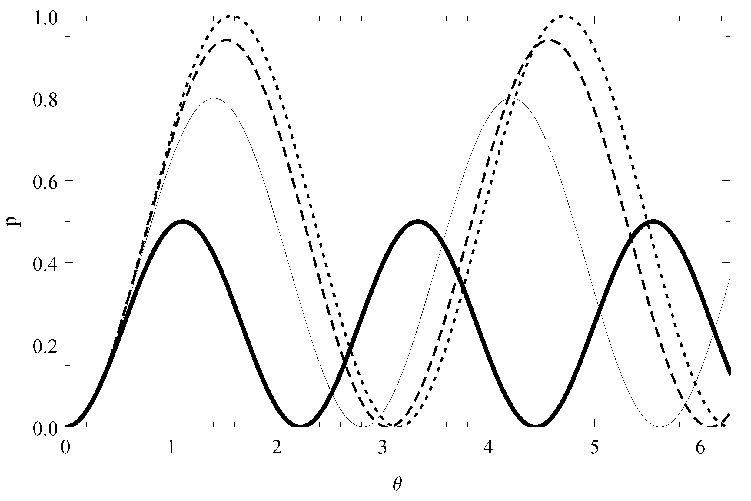
In the presence of off-resonance effects, the success probability of the various quantum strategies is affected both in terms of amplitude and periodicity. In particular, focusing on the constant driving case, the success probability $p_0\left(\theta \right)$ in Equation (42) is dampened by the Lorentzian-like factor $1/(1+{\beta }_0^2)$. Moreover, the periodicity of the oscillations of this probability changes from $2\pi$ to $2\pi /{\left(1+{\beta }_0^2\right)}^{\frac{1}{2}}$. In summary, oscillations become smaller in amplitude but higher in frequency. These facts are clearly visible in Figure 1.

(2)

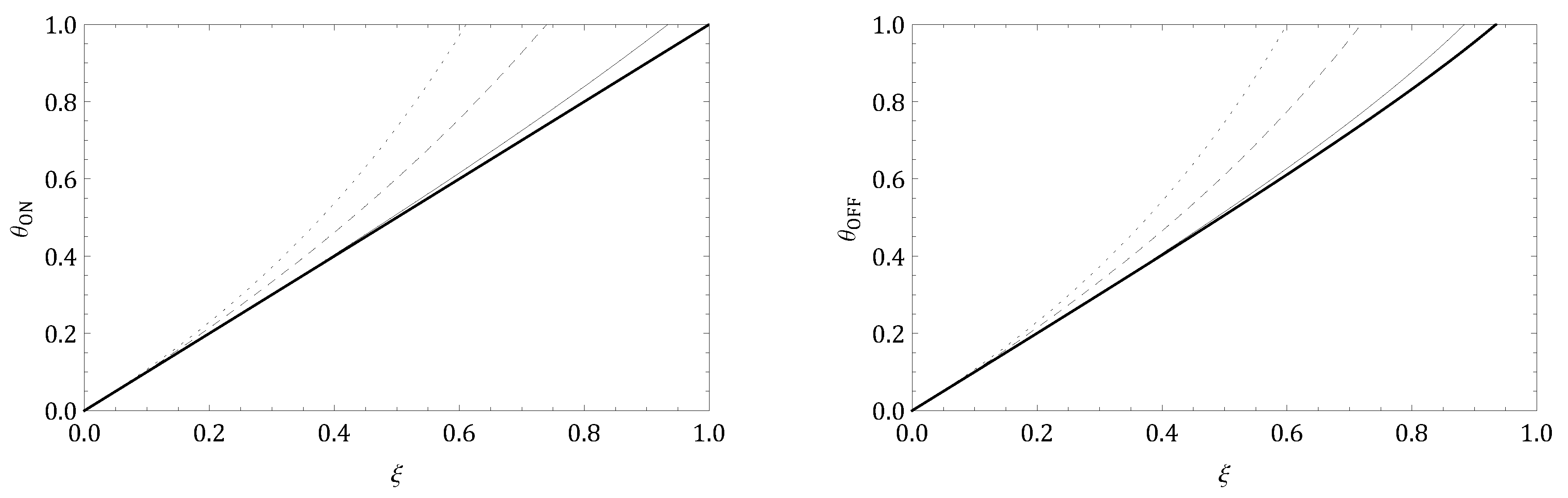
Departing from the on-resonance condition (that is, ${\beta }_0=0$), we observe a change in the geodesic paths on the underlying manifolds. The presence of off-resonance effects (that is, ${\beta }_0\ne 0$) generates geodesic paths with a more complex structure. In particular, unlike what happens when the on-resonance condition is satisfied, numerical integration of the geodesic equations is required. In particular, the numerical plots of the geodesic paths $\theta$ versus the affine parameter $\xi$ for the four driving strategies with geodesic equations in Equations (46), (53), (60) and (67) appear in Figure 2.

(3)

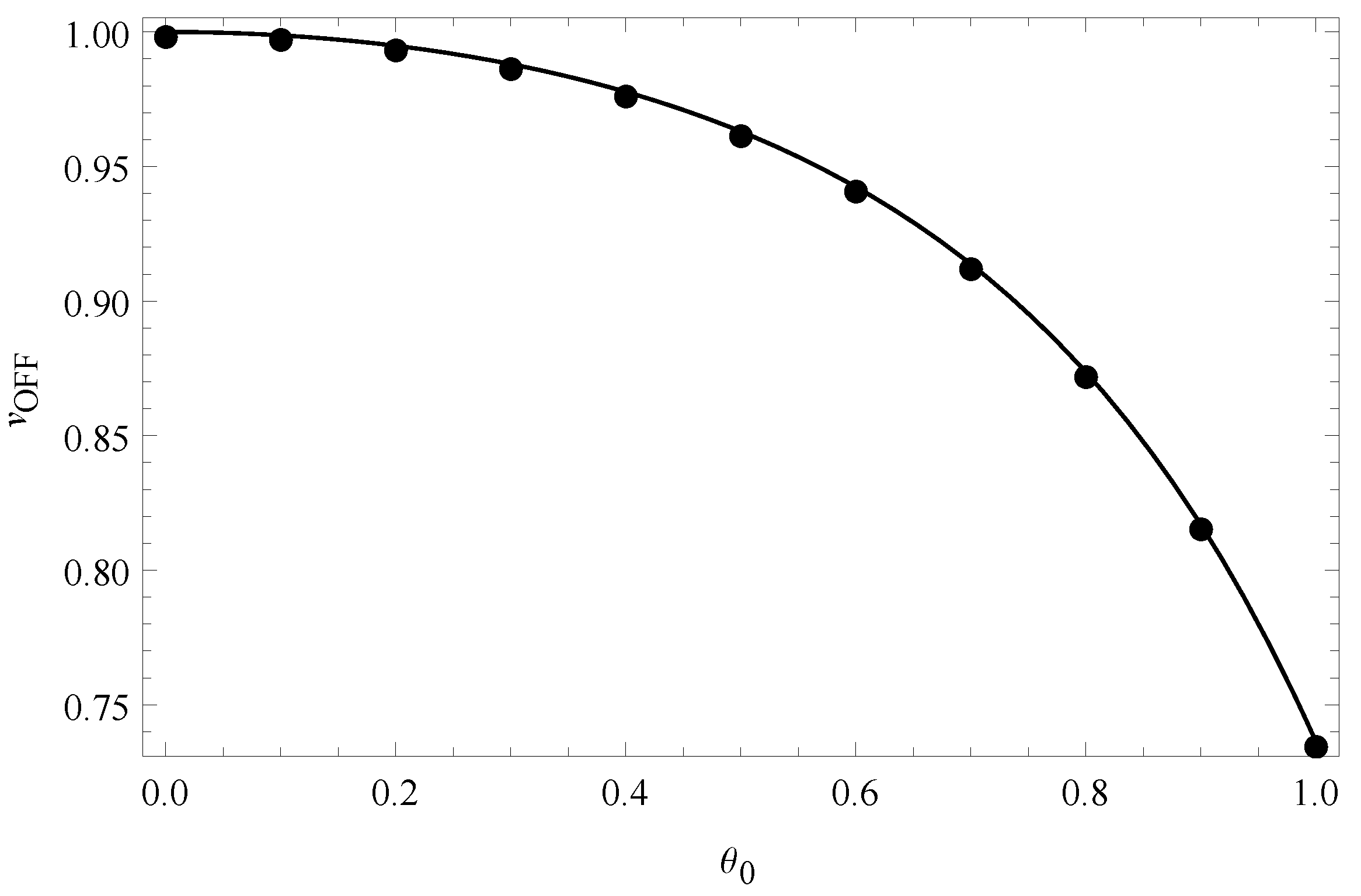
Each and every numerical value of the geodesic speeds corresponding to the various quantum driving strategies considered in this paper becomes smaller when departing from the on-resonance condition (see Figure 3, for instance). In general, quantum driving strategies characterized by a high geodesic speed appear to be very sensitive to off-resonance effects. Instead, strategies yielding geodesic paths with smaller geodesic speed values seem to be more robust against departures from the on-resonance condition. These observations can be understood from Figure 4.

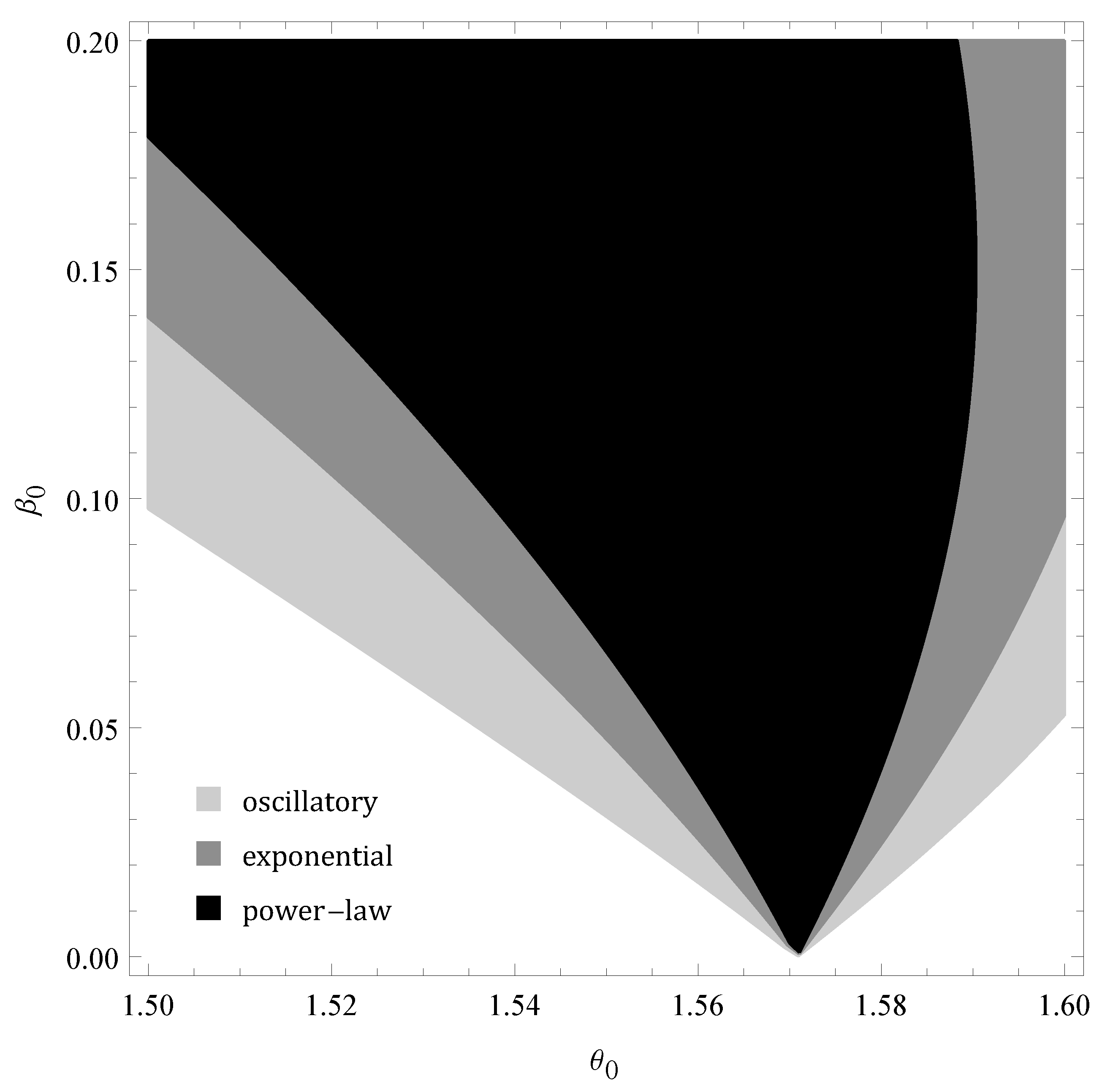
(4)

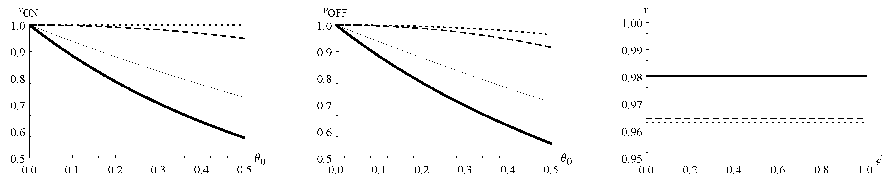
In the off-resonance regime, there emerges a sensitive dependence of the geodesic speeds on the initial conditions. This, in turn, can cause a change in the ranking of the various quantum driving strategies. In particular, the strategy specified by a constant Fisher information is no longer the absolute best strategy in terms of speed. Indeed, it is possible to find two-dimensional (2D) parametric regions where this strategy is being outperformed by all the remaining strategies both in terms of speed and robustness. In general, these 2D regions are more extended for the less robust strategies (see Equations (94) and (95)). For instance, we can identify 2D regions where the speed-based ranking becomes: (1) Oscillatory strategy; (2) exponential-law decay strategy; (3) power-law decay strategy. Instead, considering the very same 2D regions, the robustness-based ranking is given by: (1) Power-law decay strategy; (2) exponential-law decay strategy; (3) oscillatory strategy. In these 2D regions, the constant strategy is the worst, both in terms of speed and robustness. These findings are illustrated in Figure 5.

In conclusion, our information geometric analysis suggests that speed and robustness appear to be competing features when departing from the on-resonance condition. Ideally, a quantum driving strategy should be fast, robust, and thermodynamically efficient [34,35,36]. Since speed and thermodynamic efficiency quantified in terms of minimum entropy production paths seem to be conflicting properties as well [20,21], it appears reasonable to think there might be a connection between robustness and thermodynamic efficiency. We leave the exploration of this conjectured link to future scientific efforts.

References

1. Jackson, J.D. Classical Electrodynamics; John Wiley & Sons, Inc.: New York, NY, USA, 1999. [Google Scholar]
2. Sakurai, J.J. Modern Quantum Mechanics; Addison-Wesley Publishing Company, Inc.: Boston, MA, USA, 1994. [Google Scholar]
3. D’Alessandro, D.; Dahleh, M. Optimal control of two-level quantum systems. IEEE Trans. Autom. Control 2001, 46, 866. [Google Scholar] [CrossRef]
4. Boscain, U.; Charlot, G.; Gauthier, J.-P.; Guerin, S.; Jauslin, H.-R. Optimal control in laser-induced population transfer for two- and three-level quantum systems. J. Math. Phys. 2002, 43, 2107. [Google Scholar] [CrossRef]
5. Romano, R. Geometric analysis of minimum-time trajectories for a two-level quantum system. Phys. Rev. A 2014, 90, 062302. [Google Scholar] [CrossRef] [Green Version]
6. Byrnes, T.; Forster, G.; Tessler, L. Generalized Grover’s algorithm for multiple phase inversion states. Phys. Rev. Lett. 2018, 120, 060501. [Google Scholar] [CrossRef] [Green Version]
7. Cafaro, C.; Alsing, P.M. Continuous-time quantum search and time-dependent two-level quantum systems. Int. J. Quantum Inf. 2019, 17, 1950025. [Google Scholar] [CrossRef]
8. Aharonov, Y.; Anandan, J.; Popescu, S.; Vaidman, L. Superpositions of time evolutions of a quantum system and a quantum time-translation machine. Phys. Rev. Lett. 1990, 64, 2965. [Google Scholar] [CrossRef] [Green Version]
9. Kempf, A.; Prain, A. Driving quantum systems with Superoscillations. J. Math. Phys. 2017, 58, 082101. [Google Scholar] [CrossRef]
10. Barredo, D.; Labuhn, H.; Ravets, S.; Lahaye, T.; Browaeys, A. Coherent excitation transfer in a spin chain of three Rydberg atoms. Phys. Rev. Lett. 2015, 114, 113002. [Google Scholar] [CrossRef] [Green Version]
11. Schempp, H.; Gunter, G.; Wuster, S.; Weidemuller, M.; Whitlock, S. Correlated exciton transport in Rydberg-dressed-atom spin chains. Phys. Rev. Lett. 2015, 115, 093002. [Google Scholar] [CrossRef]
12. Shi, Z.C.; Wang, W.; Yi, X.X. Population transfer driven by off-resonant fields. Opt. Express 2016, 24, 21971. [Google Scholar] [CrossRef] [Green Version]
13. Hirose, M.; Cappellaro, P. Time-optimal control with finite bandwidth. Quantum Inf. Process. 2018, 17, 88. [Google Scholar] [CrossRef] [Green Version]
14. Allen, L.; Eberly, J.H. Optical Resonance and Two-Level Atoms; Dover Publications: New York, NY, USA, 1987. [Google Scholar]
15. Laucht, A.; Simmons, S.; Kalra, R.; Tosi, G.; Dehollain, J.P.; Muhonen, J.T.; Freer, S.; Hudson, F.E.; Itoh, K.M.; Jamieson, D.N.; et al. Breaking the rotating wave approximation for a strongly driven dressed single-electron spin. Phys. Rev. B 2016, 94, 161302. [Google Scholar] [CrossRef] [Green Version]
16. Dai, K.; Wu, H.; Zhao, P.; Li, M.; Liu, Q.; Xue, G.; Tan, X.; Yu, H.; Yu, Y. Quantum simulation of the general semi-classical Rabi model in regimes of arbitrarily strong driving. Appl. Phys. Lett. 2017, 111, 242601. [Google Scholar] [CrossRef]
17. Cafaro, C.; Alsing, P.M. Theoretical analysis of a nearly optimal analog quantum search. Phys. Scr. 2019, 94, 085103. [Google Scholar] [CrossRef] [Green Version]
18. Gassner, S.; Cafaro, C.; Capozziello, S. Transition probabilities in generalized quantum search Hamiltonian evolutions. Int. J. Geom. Methods Mod. Phys. 2020. accepted. [Google Scholar] [CrossRef]
19. Farhi, E.; Gutmann, S. Analog analogue of a digital quantum computation. Phys. Rev. A 1998, 57, 2403. [Google Scholar] [CrossRef] [Green Version]
20. Cafaro, C.; Alsing, P.M. Decrease of Fisher information and the information geometry of evolution equations for quantum mechanical probability amplitudes. Phys. Rev. E 2018, 97, 042110. [Google Scholar] [CrossRef] [PubMed] [Green Version]
21. Cafaro, C.; Alsing, P.M. Information geometry aspects of minimum entropy production paths from quantum mechanical evolutions. Phys. Rev. E 2019, in press. [Google Scholar]
22. Messina, A.; Nakazato, H. Analytically solvable Hamiltonians for quantum two-level systems and their dynamics. J. Phys. A Math. Theor. 2014, 47, 445302. [Google Scholar] [CrossRef] [Green Version]
23. Grimaudo, R.; de Castro, A.S.M.; Nakazato, H.; Messina, A. Classes of exactly solvable generalized semi-classical Rabi systems. Ann. Phys. 2018, 2018, 1800198. [Google Scholar] [CrossRef] [Green Version]
24. Braunstein, S.L.; Caves, C.M. Statistical distance and geometry of quantum states. Phys. Rev. Lett. 1994, 72, 3439. [Google Scholar] [CrossRef] [PubMed]
25. Berry, M.V. Quantal phase factors accompanying adiabatic changes. Proc. R. Soc. Lond. A 1984, 392, 45. [Google Scholar]
26. Aharonov, Y.; Anandan, J. Phase change during a cyclic quantum evolution. Phys. Rev. Lett. 1987, 58, 1593. [Google Scholar] [CrossRef] [PubMed]
27. Resta, R. Manifestations of Berry’s phase in molecules and condensed matter. J. Phys. Condens. Matter 2000, 12, R107. [Google Scholar] [CrossRef]
28. Braunstein, S.L.; Caves, C.M.; Milburn, G.J. Generalized uncertainty relations: Theory, examples, and Lorenz Invariance. Ann. Phys. 1996, 247, 135. [Google Scholar] [CrossRef] [Green Version]
29. Cafaro, C.; Mancini, S. An information geometric viewpoint of algorithms in quantum computing. AIP Conf. Proc. 2012, 1443, 374. [Google Scholar]
30. Cafaro, C.; Mancini, S. On Grover’s search algorithm from a quantum information geometry viewpoint. Physica A 2012, 391, 1610. [Google Scholar] [CrossRef] [Green Version]
31. Cafaro, C. Geometric algebra and information geometry for quantum computational software. Physica A 2017, 470, 154. [Google Scholar] [CrossRef] [Green Version]
32. Amari, S.; Nagaoka, H. Methods of Information Geometry; Oxford University Press: Providence, RI, USA, 2000. [Google Scholar]
33. Felice, D.; Cafaro, C.; Mancini, S. Information geometric methods for complexity. Chaos 2018, 28, 032101. [Google Scholar] [CrossRef]
34. Castelvecchi, D. Clash of the physical laws. Nature 2017, 543, 597. [Google Scholar] [CrossRef] [Green Version]
35. Faist, P.; Renner, R. Fundamental work cost of quantum processes. Phys. Rev. X 2018, 8, 021011. [Google Scholar] [CrossRef] [Green Version]
36. Campbell, S.; Deffner, S. Trade-off between speed and cost in shortcuts to adiabaticity. Phys. Rev. Lett. 2017, 118, 100601. [Google Scholar] [CrossRef] [PubMed] [Green Version]
37. Lee, J.M. Riemannian Manifolds: An Introduction to Curvature; Springer: New York, NY, USA, 1997. [Google Scholar]
Figure 1. Plot of the success probability p versus the temporal parameter θ in the case of constant driving for β = 0 (dotted), β 0 = 0.25 (dashed), β 0 = 0.5 (thin solid), and β 0 = 1 (thick solid).
Quantumrep 02 00011 g001
Figure 2. Numerical plots of the geodesic paths θ versus the affine parameter ξ for the four driving strategies: Power-law (dotted line), exponential (dashed line), oscillatory (thin solid line), and constant (thick solid line). In the LHS (left-hand-side), we consider the on-resonance scenario with β 0 = 0 . In the RHS (right-hand-side), we consider the off-resonance scenario with β 0 = 1 / 2 . In both sides, we set Γ / ħ = 1 , λ = 2 / π , θ 0 = 0 , and θ ˙ 0 = 1 .
Quantumrep 02 00011 g002
Figure 3. Plot of the analytical (thin solid) and numerical (filled circle) values of the geodesic speed v OFF versus the initial condition θ 0 in the case of constant driving. In the plot, we set β 0 = 1 / 2 , Γ / ħ = 1 , and θ ˙ 0 = 1 .
Quantumrep 02 00011 g003
Figure 4. From left to right: (L) Plot of the geodesic speed v ON versus the initial condition θ 0 with β 0 = 0 ; (C) Plot of the geodesic speed v OFF versus the initial condition θ 0 with β 0 = 1 / 2 ; (R) Plot of the robustness coefficient r versus the affine parameter ξ . Plots that correspond to the constant, oscillatory, exponential decay, and power law decay strategies appear in dotted, dashed, thin solid, and thick solid lines, respectively. In all plots, we set Γ / ħ = 1 , λ = 2 / π , and θ ˙ 0 = 1 .
Quantumrep 02 00011 g004
Figure 5. Plot of the two-dimensional parametric regions P β 0 , θ 0 where the oscillatory (light grey), the exponential decay (grey), and the power law decay (black) driving strategies outperform the constant driving scheme in terms of both geodesic speed and robustness. Note that the light grey region contains the grey region while the grey region contains the black region. Furthermore, the black region specifies a driving strategy more robust than that specified by the grey region while the grey region specifies a driving strategy more robust than that specified by the light grey region. In all region plots, we set Γ / ħ = 1 , λ = 2 / π , and θ ˙ 0 = 1 . Finally, the maximum success probability of each driving scheme is assumed to be greater than 25 / 26 0.96 , that is, 0 β 0 0.20 .
Quantumrep 02 00011 g005