Article

Robust Path Tracking Control with Lateral Dynamics Optimization: A Focus on Sideslip Reduction and Yaw Rate Stability Using Linear Quadratic Regulator and Genetic Algorithms

by
Karrar Y. A. Al-bayati
1,2,*,
Ali Mahmood
1,3 and
Róbert Szabolcsi
4
1
Doctoral School on Safety and Security Sciences, Óbuda University, 1081 Budapest, Hungary
2
Electronic and Communication Engineering Department, University of Kufa, Najaf 54001, Iraq
3
Systems and Control Engineering Department, Ninevah University, Mosul 41001, Iraq
4
Kandó Kálmán Faculty of Electrical Engineering, Óbuda University, 1034 Budapest, Hungary
*
Author to whom correspondence should be addressed.
Vehicles 2025, 7(2), 50; https://doi.org/10.3390/vehicles7020050
Submission received: 16 March 2025 / Revised: 28 April 2025 / Accepted: 10 May 2025 / Published: 21 May 2025

Abstract

:
Currently, one of the most important challenges facing autonomous vehicles’ development due to varying driving conditions is effective path tracking while considering lateral stability. To address this issue, this study proposes the optimization of the linear quadratic regulator (LQR) control system by using the genetic algorithm (GA) to support the vehicle in following the predefined path accurately, minimizing the sideslip, and stabilizing the vehicle’s yaw rate. The dynamic system model of the vehicle is represented based on yaw rate angle, lateral speed, and vehicle sideslip angle as the variables of the state space model, with the steering angle as an input parameter. Using the GA to optimize the LQR control by tuning the weighting of the Q and R matrices led to enhancing the system response and minimizing deviation errors via a proposed cost function of GA. The simulation results were obtained using MATLAB/Simulink 2024a, with a representation of a predefined path as a Gaussian path. Under external and internal disturbances, such as road conditions, lateral wind, and actuator delay, the model demonstrates improved tracking performance and reduced sideslip angle and lateral acceleration by adjusting the longitudinal vehicle speed. This work highlights the effectiveness of robust control in addressing path planning, driving stability, and safety in autonomous vehicle systems.

1. Introduction

Recently, there has been widespread interest in developing the autonomous vehicle sector due to the increasing number of vehicles and changing driving conditions. This has contributed to improved performance, driving safety, and comfort, in addition to preventing deviation from the predetermined path and addressing traffic congestion at intersections [1,2,3,4]. Path tracking is one of the most prominent challenges in the field of autonomous vehicles in terms of accuracy, reducing the risk of deviation and increasing the comfort of passengers [5,6,7]. It has become necessary to use control strategies, especially when changing speed, maneuvering during lane changes, and turning at various steering angles. Many approaches have been adopted to address path tracking issues, such as traditional proportional–integral–derivative (PID), fuzzy logic control (FLC), model predictive control (MPC), and linear quadratic regulators (LQRs), based on different parameters—for instance, lateral forces and sideslip angle [8,9,10,11,12,13]. Many researchers have adopted the PID control technique to ensure the accuracy of the predicted path tracking relative to the actual path [14,15]. Zhaojian Wang et al. applied a PID controller based on a simplified two-DOF vehicle model to reduce the lateral deviation by modifying the steering angle [16]. Tiep et al. used the fuzzy approach for tuning the PID parameters, which showed a good response, stability, and accuracy of addressing lateral deviation issues compared to the classical PID [17]. Gaining Han et al. proposed a neural network PID controller using the CARMA model to represent the second order of the vehicle’s dynamic model. It demonstrated an effective path tracking response with an approximately 2-m error in actual position and a 3-degree error in the heading angle of the vehicle, which outperformed the fuzzy-PID controller [18].
Some researchers applied alternative control methods instead of the PID controller due to the difficulty in handling nonlinear systems [19,20,21]. A model predictive controller (MPC) was presented by Hengyang Wang et al. for the precise tracking process of an autonomous vehicle. They improved the MPC controller by specifying the optimal cost weights using the FLC controller to ensure not only tracking accuracy but also system stability [22]. Juqi et al. demonstrated the effectiveness of path tracking, focusing on the sharp steering angle changes based on the expected value of the heading angle and speed using the fuzzy-MPC [23]. However, several research projects have been conducted using the LQR controller, which demonstrates a dynamic response under varying road conditions to minimize the lateral force error and tracking instability along the actual predefined path [24,25]. Zhao et al. employed an adaptive prediction time linear quadratic regulator (APT-LQR) algorithm to stabilize the performance of the vehicle dynamic system by optimizing the front-wheel steering angle and specifying a desired yaw moment for each wheel. Despite not considering tire slip force and driving speed variation, they showed robust control and stability in following the actual path [26]. Zhaoqiang et al. utilized the Fuzzy Logic Controller to adjust the coefficient values of the LQR controller. Their results show an improvement in accuracy within 0.2 m of lateral error, approximately at low-speed path tracking, while at high speed, the proposed LQR controller minimizes the lateral error by approximately 28%, making it more precise and stable than the MPC controller, especially at low vehicle speeds [27]. Several recent studies have shown that combining LQR with intelligent technologies can improve the performance of control systems. In one study, a neural network-based dynamic model was used within an LQR to track vehicle trajectories [28], while another study combined PSO and GA to enhance LQR performance in an active suspension system [29]. These results confirm the benefits of combining LQR with modern optimization methods.
Despite the improvements in the above-mentioned path tracking control strategies such as fuzzy-LQR, they have sensitivity toward uncertainties due to their adopted rules or prediction strategies. These models also did not take into consideration the parameters of lateral forces, the yaw moment, and the sideslip angle. This study proposes an advanced control approach of using a genetic algorithm (GA) with an LQR controller in parallel, not only for comprehensive path tracking accuracy but also for vehicle stability. The dynamic model of the vehicle is derived based on lateral velocity, yaw rate, and sideslip angle as state space variables, with the steering angle as an input variable. To achieve optimal performance in precise path tracking, lateral stability, and computational control effort, the GA was utilized to specify the value of the LQR matrices under road environment variation dynamically. The simulation results of the proposed LQR with the GA show effective performance in path tracking accuracy, sideslip reduction based on the desired yaw rate, and lateral acceleration minimization by adjusting the longitudinal vehicle speed with and without disturbances. This work demonstrates the significant progress of trajectory planning through the robust, advanced LQR-GA control, showing that the model successfully maintains vehicle stability and safety by reducing lateral forces and sideslip angle. The schematic diagram in Figure 1 illustrates the structure of the LQR-GA control for vehicle path tracking.
This paper is organized as follows: the state-space formulation of the vehicle dynamic model is presented in Section 2. Section 3 details the optimization of the LQR control technique using GA, with mean squared error (MSE) as the cost function to reduce lateral forces on the vehicle. In Section 4, the simulation results are presented using the Simulink program under various scenarios. First, the LQR-GA is applied for vehicle path tracking. Then, the longitudinal vehicle speed is used as a variable to maintain lateral acceleration within safe limits, ensuring vehicle stability, comfort, and safety. Finally, lateral wind force, slippery road conditions, and actuator delay are considered as internal and external disturbances. Section 5 concludes the proposed work.

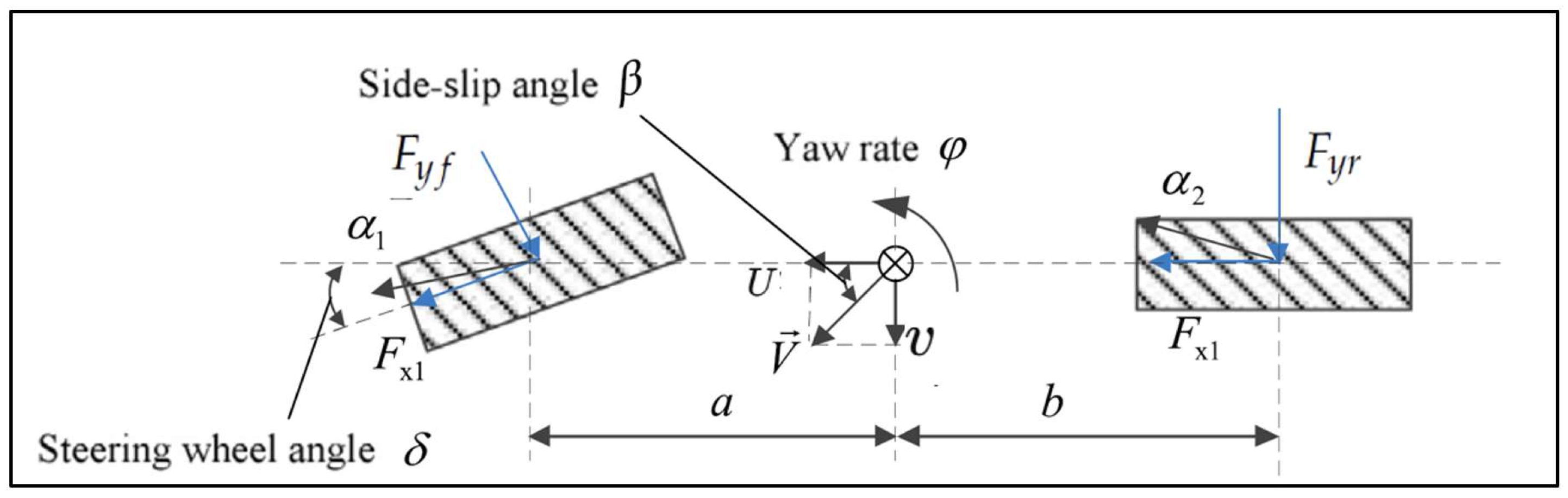
2. Vehicle Dynamics Modeling
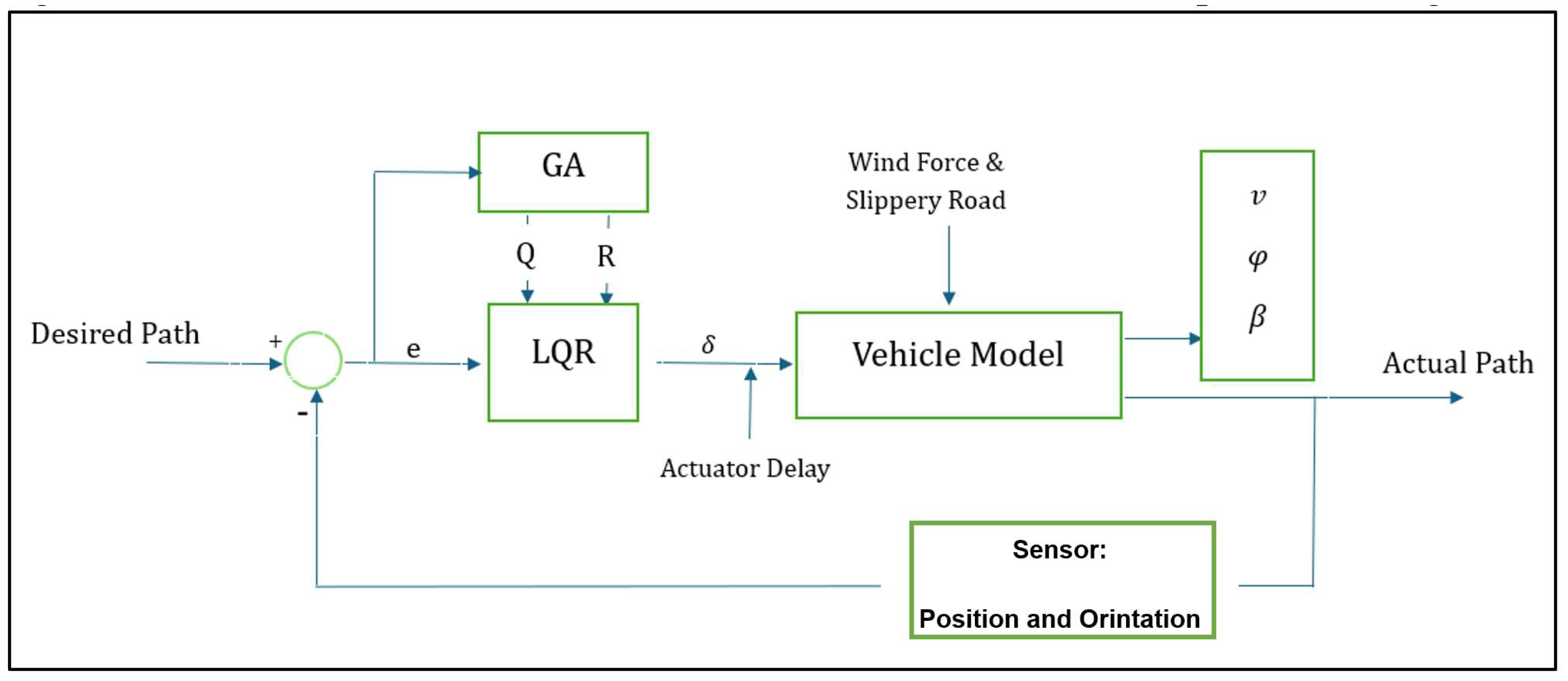
To mathematically derive the four-wheel vehicle dynamic model, the process begins with a simplified 2-DOF vehicle model due to the complexity of nonlinear steering control. In Figure 2, by applying Newton’s second law, the lateral motion and rotational motion equations of the vehicle are obtained as follows [30]:
F y = m a y = F y f cos δ + F y r
M = I z φ ˙ = a F y f cos δ b F y r
In general, the steering angle is assumed to be small, which leads to simplifying the above-mentioned equations as follows:
F y = m a y = F y f + F y r
M = I z φ ˙ = a F y f b F y r
The lateral force can be regarded as a linear relationship of the tire sideslip angle based on the 2-DOF vehicle model [31]. The lateral force and lateral acceleration in Equation (3) can be represented as follows, respectively:
F y i = C α i
a y = v ˙ + φ U
where C and α i are the lateral cornering stiffness and sideslip angle of the tire, respectively. According to [26,27,32], the lateral slip angle can be represented as:
α f = δ + v + a φ U
α r = v b φ U
By combining 5–8 equations in Equations (3) and (4), we obtain the following eq as:
v ˙ = U φ 2 C f + C r m U v + 2 a C f b C r m U φ + 2 C f m δ
φ ˙ = 2 a C f I z δ 2 a C f + b C r I z U v 2 a 2 C f + b 2 C r I z U φ
The sideslip angle is a key parameter in the dynamic model, representing the angle between the longitudinal speed of the vehicle and its speed vector. The following equation expresses the sideslip angle [31,33]:
β = arctan ( v U )
For approximation, β << 1
β v U
By deriving the sideslip angle Equation (12) and combining it with lateral velocity Equation (9), the sideslip angle dynamics are as follows:
β ˙ = 2 C f + C r m U β 1 + 2 a C f b C r m U 2 φ + 2 C f m U δ
To represent the state space of vehicle dynamics, three parameters are used based on the above-mentioned equations. The three state variables are lateral velocity, yaw rate and sideslip angle, while the control input is the steering angle. The state space concluded from differential Equations (9), (10) and (13) can be written as:
x ˙ = A x + B u
where:
A = 2 C f + C r m U 0 1 2 a C f b C r m U 2 0 2 C f + C r m U U + 2 a C f b C r m U 0 2 a C f + b C r I z U 2 a 2 C f + b 2 C r I z U ,   B = 2 C f m U 2 C f m 2 a C f I z

3. Control Design

This section provides a detailed discussion on the design of the linear quadratic regulator (LQR) controller, explaining its structure and how it achieves optimal control performance. Moreover, it introduces the motivation and justification for integrating the genetic algorithm to optimize LQR parameters, highlighting the resulting advantages in system robustness and stability. The discussion highlights the rationale for selecting GA, its advantages in handling complex optimization problems, and its role in enhancing the effectiveness of the LQR controller.

3.1. Linear Quadratic Regulator (LQR)

The linear quadratic regulator (LQR) controller is a state-feedback control technique designed to minimize a quadratic cost function by optimizing the weighting matrices [34,35]. Figure 3 illustrates the block diagram of the LQR controller.
The controller operates based on the state-space representation of the vehicle dynamics system, where the state vector comprises the sideslip angle ( β ), yaw rate ( φ ), and lateral velocity ( v ).
The LQR controller minimizes the following cost function
J = 0 ( x T Q x + u T R u ) d t
where:
x is the state vector [ v , φ , β ] T
u is the control input (steering angle δ)
Q is a positive semi-definite matrix penalizing deviation in the states
R is a positive definite matrix penalizing control effort.
To solve the Algebraic Riccati equation, the optimal feedback matrix K will be used.
u = k x + φ d  
where φ d is the desired yaw rate derived from the trajectory.
The state-space representation of the LQR controller for a continuous-time linear time-invariant system is as follows:
x   ˙ t = A   x t + B   u ( t )
where:
A is the state matrix
B is the input matrix.
The quadratic cost function to be minimized is given by:
J = 0 ( x T t Q x t + u T t R u ( t ) ) d t
where:
Q is the state cost matrix; R is the control cost matrix.
By finding the optimal values of the Q and R matrices using the GA optimization algorithm, the controller gain matrix K can be computed by solving the continuous-time algebraic Riccati equation:
A T P + P A P B R 1 B T P + Q = 0
Once P is obtained, the control input is given by:
u t = R 1 B T P x ( t )
The state feedback matrix K is then given by:
K = R 1 B T P
However, the performance of the LQR controller is heavily dependent on the proper selection of the Q and R matrices. Traditional manual tuning of these matrices can be subjective, time-consuming, and may not guarantee optimal vehicle performance, particularly under complex or varying driving conditions. Therefore, an optimization method is necessary to systematically and efficiently determine the optimal weighting matrices for achieving the desired stability and path tracking performance.

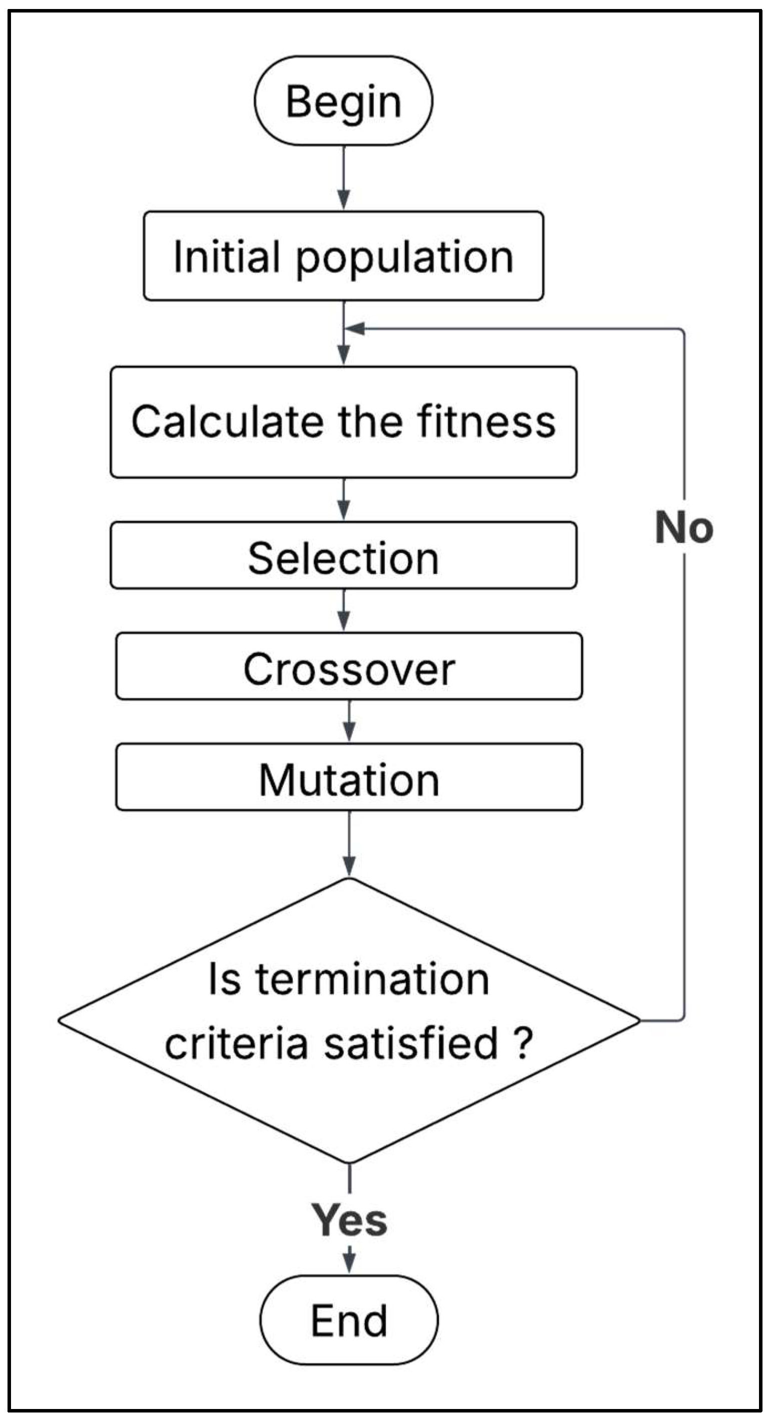
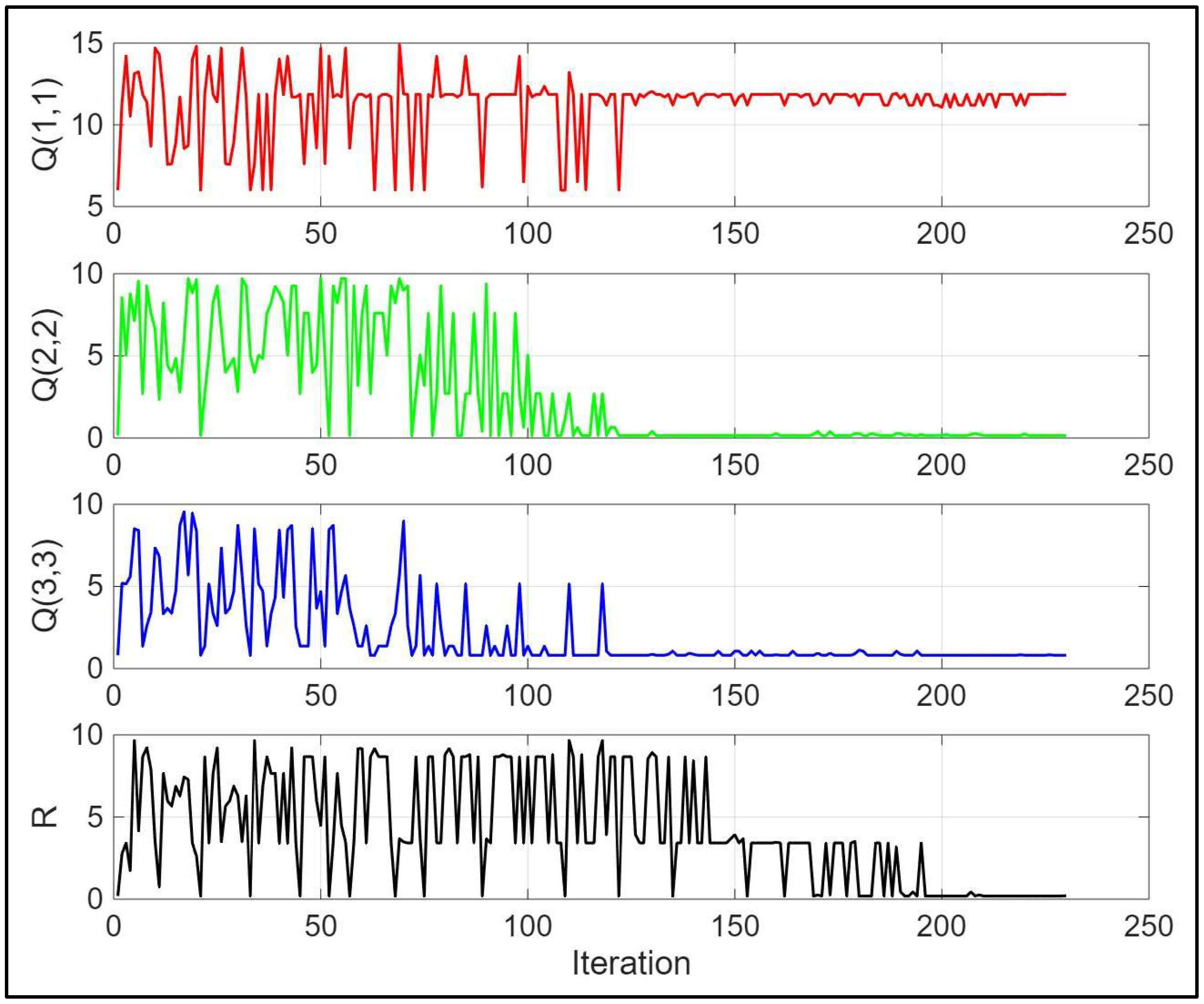
3.2. Genetic Algorithm Optimization

The genetic algorithm was initially introduced by John Holland [36,37] as a means to improve the efficiency of computational processes. The fundamental concept is inspired by the natural evolutionary process of chromosomes, starting with the representation of a chromosome’s structure [38]. This structure encompasses all elements that require optimization. For the LQR controller, the optimization process involves determining the Q and R matrices [39,40]. Once the chromosome structure is established, the GA optimization process begins, starting with the random selection of an initial population of chromosomes. At this stage, a fitness function evaluates the performance of each chromosome. Subsequently, a crossover occurs between pairs of chromosomes to exchange information and generate new ones. The final step involves mutation, where random changes are applied to some individuals in the population to introduce diversity and enhance the optimization process [41].
As the performance of the LQR controller largely depends on the values of its Q and R matrices, the GA optimization method will be used to select their parameters to minimize the trajectory tracking error and improve stability. GA is a population-based search algorithm inspired by natural selection.
The elements of Q and R matrices are encoded as genes, while the trajectory tracking error, lateral acceleration, and yaw rate deviation will be evaluated as a fitness function. It must be mentioned that Q must be positive semi-definite, and R must be positive definite.
Figure 4 shows a flowchart of the GA.
The choice of GA is justified by its flexibility in handling both discrete and continuous optimization variables as well as its robustness in noisy and dynamic environments, which are typical in autonomous vehicle operation scenarios. Moreover, the use of GA eliminates the subjectivity associated with the manual tuning of LQR parameters and ensures a more consistent and reliable control performance, as demonstrated by the convergence behavior and performance improvements in the simulation results.
By integrating GA with LQR, this study ensures that the path tracking control system is optimized not only for the nominal conditions but also maintains robustness and stability under road disturbances, actuator delays, and variable vehicle speeds.

4. Simulation Setup

The simulation is implemented in MATLAB/Simulink 2024a, utilizing a Gaussian-function trajectory to assess the vehicle’s path tracking performance and lateral stability under varying conditions. The Gaussian trajectory is defined with a mean (μ) of 280 and a standard deviation (σ) of 80. A time step (dt) of 0.01 s is employed, and the total simulation duration (T) is set to 50 s. The evaluation criteria primarily include the trajectory tracking error, defined as the deviation between the desired and actual paths; the lateral acceleration, which reflects passenger comfort and tire force dynamics; and the yaw rate, which serves as a key indicator of the vehicle’s rotational stability.
The simulation model incorporates a set of key parameters that accurately represent the physical and dynamic characteristics of the vehicle. These parameters, including the vehicle’s mass, yaw moment of inertia, center of gravity location, and tire properties, are critical for evaluating the performance of the control system. The detailed specifications used in the simulation are presented in Table 1 below [7]:

4.1. Constant vs. Variable Longitudinal Velocity U

Firstly, the performance of the LQR controller optimized by the GA will be tested at a constant longitudinal velocity of U = 15 m/s (54 km/h).
The genetic algorithm tuning process exhibited effective convergence within 50 generations, resulting in significant improvements in both stability and control performance. The optimized weighting matrices achieved a well-balanced trade-off between minimizing state deviations and limiting control effort. The stability of the closed-loop system was verified by analyzing the eigenvalues of the system matrix, all of which had negative real parts, confirming the system’s stability under the optimized control parameters. Following this stability validation, the optimized values for the weighting matrices were determined as Qdiagonal = [14.6014, 0.1536, 0.1000] and R = 0.0717.
Figure 5 demonstrates the evolution of the individual components of the Q and R matrices during the GA optimization process. The plots for Q (1,1), Q (2,2), Q (3,3), and R show significant variability in the initial iterations as the algorithm explores the solution space. As optimization progresses, the values stabilize and converge to their final optimal values, reflecting the algorithm’s ability to identify effective control parameters. This convergence behavior highlights the robustness of the GA in balancing the competing objectives of minimizing state deviations and control effort.
Figure 6 illustrates the desired trajectory and the actual path, which closely aligns with the desired Gaussian trajectory, highlighting the controller’s precision and effectiveness in maintaining accurate path tracking.
Figure 7 illustrates the lateral acceleration (ay) of the vehicle over the 50-s simulation period. Lateral acceleration is a critical parameter for evaluating passenger comfort and the forces acting on the tires during cornering and lane change maneuvers.
The results show that the GA-optimized controller maintains a consistent lateral acceleration profile without excessive peaks or abrupt changes. However, its maximum value (12.43 m/s2) under constant U is considered very high [42]. As a result, to reduce the lateral acceleration below a specific threshold, the value of U will not remain constant during the simulation but will vary depending on the lateral acceleration, as shown in Equation (22).
U v = U ( 1 g a i n × a y a y m a x )
where:
Uv: variable longitudinal velocity (m/s)
Gain: a constant value ( 0 < G a i n < 1 )
aymax: the maximum acceptable lateral acceleration (0.4 g) [43].
The lateral acceleration of the vehicle decreased from 12.43 m/s2 to 2.572 m/s2 when the longitudinal velocity U was treated as a variable. As the GA works as the optimization method, it will update the values of the Q and R parameters to keep the LQR performance as optimal so their values will become Qdiagonal = [14.9146, 0.15, 0.1] and R = [0.4833].
The steering angle behavior during the simulation provides valuable insight into the control system’s performance, highlighting its impact on vehicle stability and passenger comfort. The GA-optimized controller effectively tends to reduce peak lateral acceleration, indicating improved passenger comfort and minimized tire forces while also significantly reducing the sideslip angle, thereby enhancing lateral stability. The control input, represented by the steering angle, remained smooth and stable throughout the 50-s simulation period, avoiding oscillatory or erratic behavior.
Figure 8a presents the steering angle profile, demonstrating the controller’s ability to generate consistent and precise control inputs. The comparison between constant and variable longitudinal velocity highlights the control system’s adaptability under more realistic driving conditions.
Figure 8b depicts the yaw rate (φ) of the vehicle. The yaw rate is a crucial indicator of the vehicle’s rotational stability and its ability to follow the desired trajectory during cornering maneuvers. The results demonstrate a consistent and stable yaw rate response under the influence of the GA-optimized controller. The absence of oscillatory or abrupt changes highlights the controller’s effectiveness in maintaining the desired rotational dynamics and ensuring stability throughout the simulation. The figure also illustrates the behavior under variable longitudinal velocity, where the response remains within acceptable bounds, indicating the robustness of the controller.
Figure 8c illustrates the sideslip angle (β) of the vehicle over the 50-s simulation period. The sideslip angle represents the angular deviation between the vehicle’s velocity vector and its longitudinal axis, serving as a critical measure of lateral stability. The results demonstrate that the sideslip angle remains within a narrow range throughout the simulation, with a peak value of less than approximately 0.04 radians. This indicates effective lateral control and minimal sliding during the maneuver. The optimized LQR controller ensures that the sideslip angle returns to near zero after transient deviations, reflecting the system’s ability to maintain stability and align the vehicle’s motion with the desired trajectory. The inclusion of variable longitudinal velocity continues to reflect satisfactory performance, albeit with slightly different transient dynamics.
Figure 8d illustrates the lateral velocity v, which represents the vehicle’s velocity component perpendicular to its longitudinal direction and serves as a crucial parameter in evaluating lateral stability and handling performance. The results indicate that the lateral velocity remains well regulated throughout the maneuver, exhibiting minimal fluctuations and settling within a stable range. When variable longitudinal velocity is introduced, the results continue to support the effectiveness of the GA-optimized control strategy in maintaining stability and control.
Figure 9 illustrates the dynamic distribution of lateral forces on the front and rear axles, which are critical for maintaining stability and ensuring effective cornering performance. The GA-optimized controller ensures that these forces remain within acceptable limits, avoiding excessive peaks that could compromise tire performance or vehicle control. The smooth and consistent variation in lateral forces reflects the controller’s ability to maintain balance and stability under varying dynamic conditions. When the value of U was treated as a variable, the maximum lateral force dropped from 7715 N and 4728 N to 3421 N and 545.7 N for the front and rear tires, respectively.
As the longitudinal velocity profile was adapted as a function of lateral acceleration to enhance vehicle stability and passenger comfort during lateral maneuvers, the velocity exhibits a clear pattern of reduction followed by an increase during two main phases of the simulation (Figure 10).
This behavior results from the application of the control law defined in Equation (22), which adjusts the longitudinal velocity proportionally to the experienced lateral acceleration. Although the velocity changes by nearly a factor of two over intervals of approximately 10–12 s, this variation is smooth and progressive, corresponding to mild acceleration and deceleration rates that are well within the thresholds considered comfortable for passengers. Moreover, the reduction in lateral acceleration achieved through this strategy significantly improves ride quality by minimizing abrupt lateral forces and body sway. Therefore, the observed speed variation is both acceptable and beneficial, ensuring enhanced stability and a more comfortable experience for vehicle occupants during dynamic maneuvers.

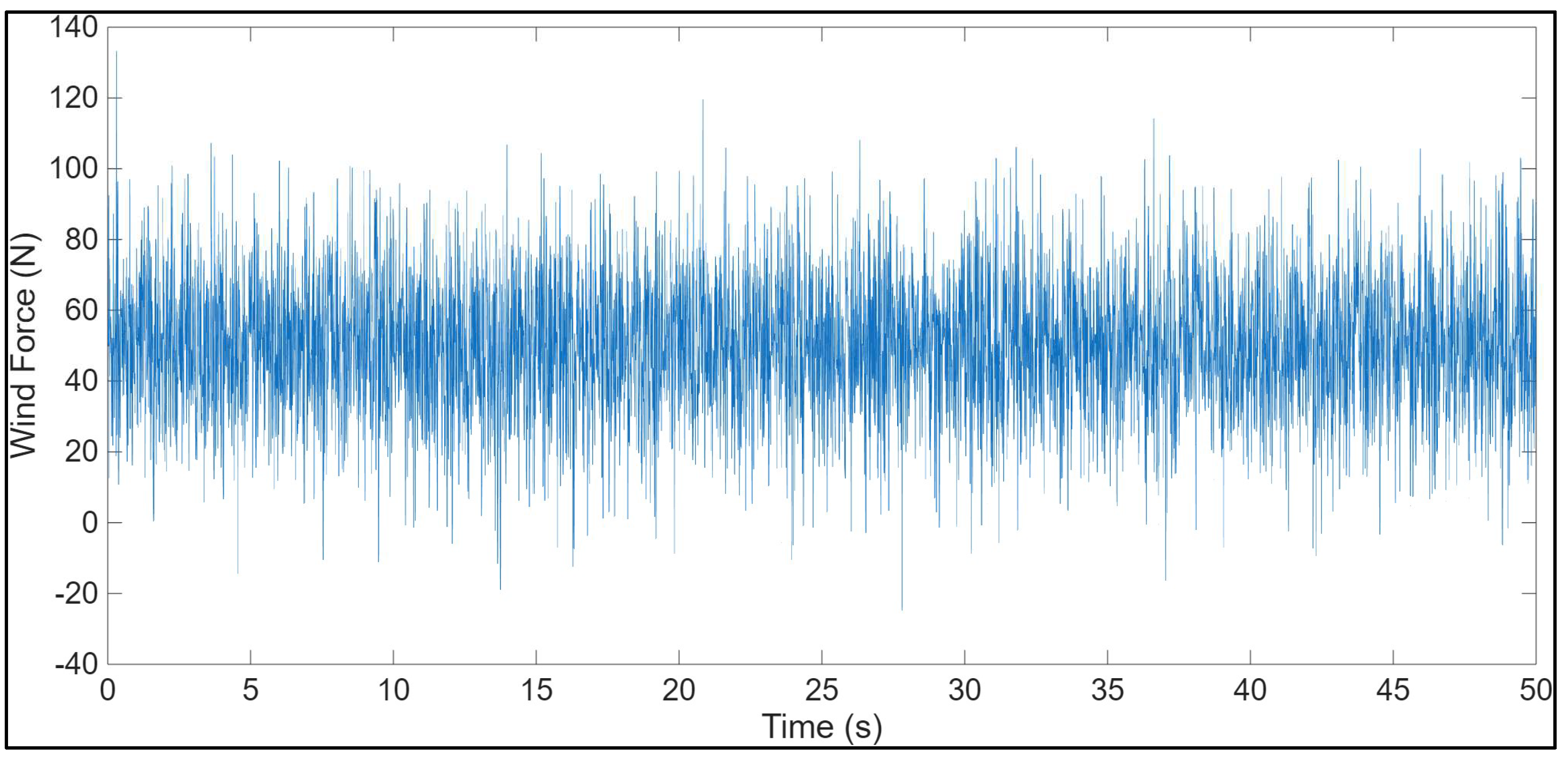
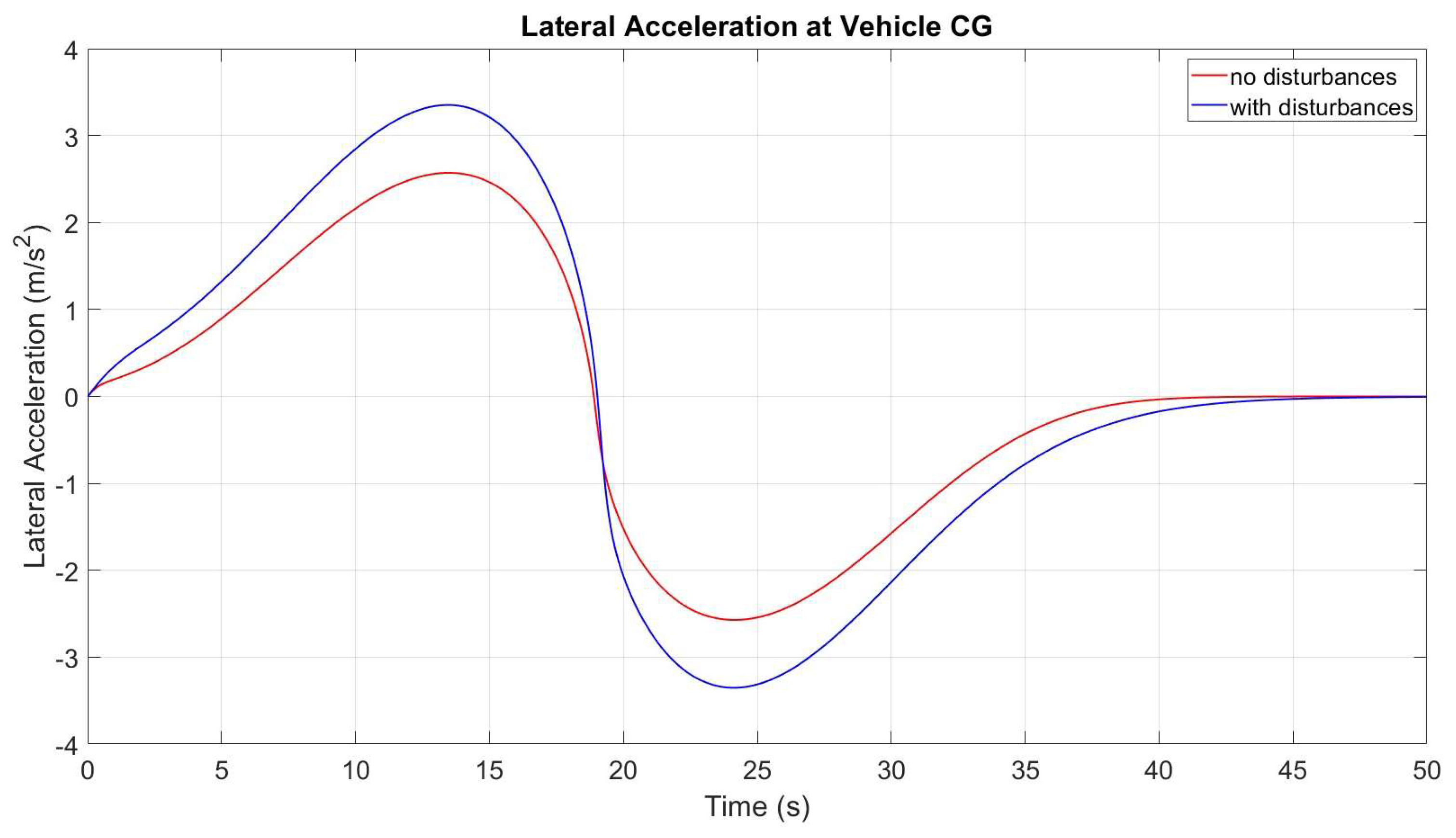
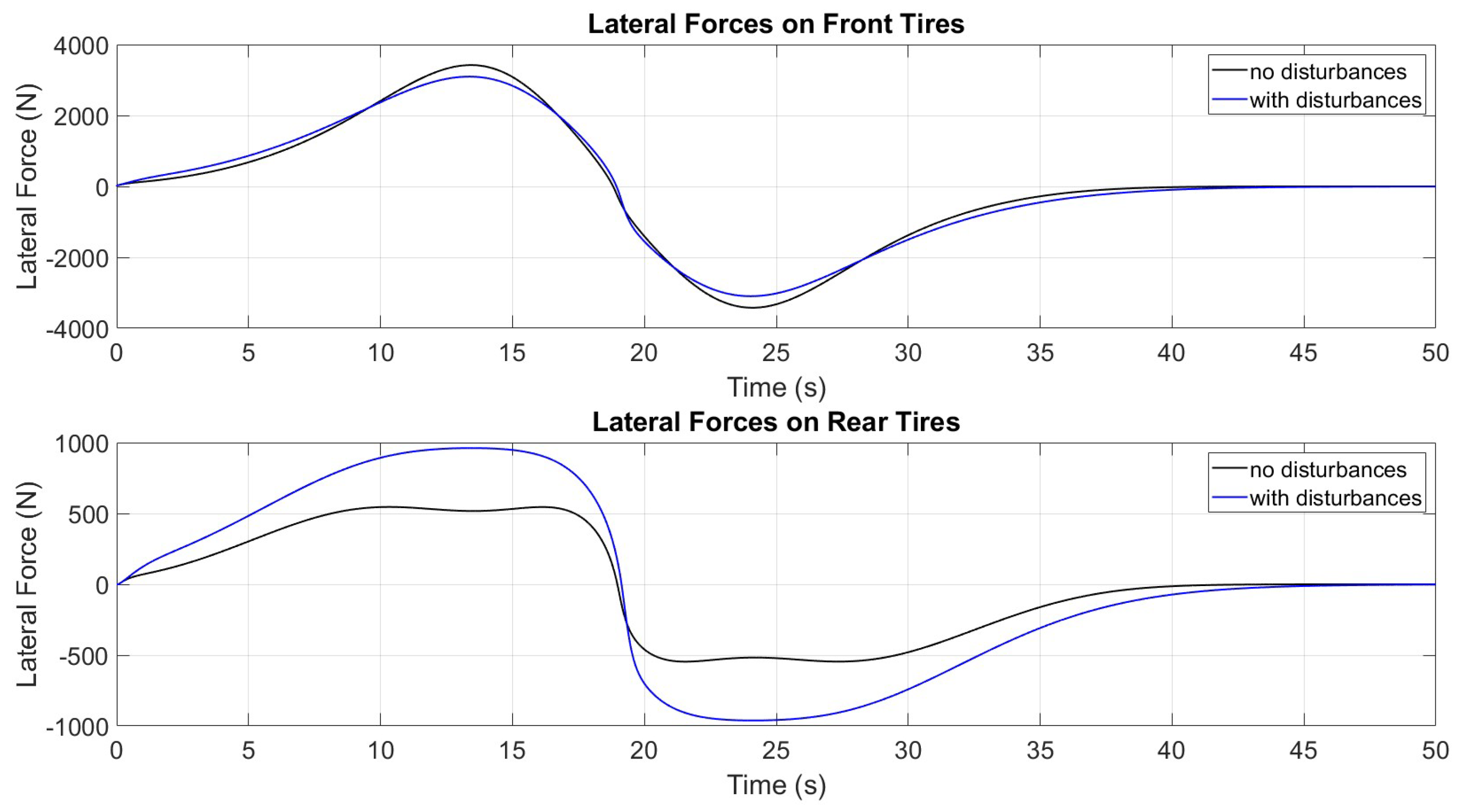
4.2. Disturbance and Delay in the Actuator Added to the System

To ensure the robustness of the designed controller, external disturbances will be added to the vehicle model. Two such disturbances are introduced: the “change in the cornering stiffness” due to slippery roads and wet road conditions, and lateral wind force. The cornering stiffness values of the front and rear wheels will be reduced to 75% of their values, while the applied lateral wind force is modeled as a random signal, with a mean value of 50 and a standard deviation of 20, as shown in Figure 11.
Finally, as an internal disturbance (uncertainties), a delay will be added to the actuator (steering input) to further test the robustness of the designed controller. This delay will be modeled as a first-order low-pass filter with a time constant (τ) of 0.5 s.
Figure 12 shows the new values of the parameters shown in Figure 8 after adding external and internal disturbances to the system.
Figure 13 shows the updated value of the lateral acceleration after adding external and internal disturbances. The previous value was 2.572 m/s2, while the new value increased to 3.352 m/s2, indicating a rise in lateral forces. However, this change remains within an acceptable range, suggesting that the controller can still maintain stable and safe vehicle behavior under disturbance conditions.
Figure 14 shows the updated values of the lateral forces after making the longitudinal velocity variable and introducing both external and internal disturbances.

5. Conclusions

This study presented an advanced path tracking control approach, integrating a linear quadratic regulator (LQR) controller with genetic algorithm optimization to enhance vehicle lateral dynamics. The proposed method focused on minimizing trajectory tracking errors, reducing sideslip angles, and ensuring yaw rate stability. Through GA optimization, the weighting matrices of the LQR controller were fine-tuned, resulting in a balanced trade-off between minimizing state deviations and limiting control effort.
The simulation results demonstrated the effectiveness of the GA-optimized controller in improving vehicle stability and control performance. The optimized controller achieved precise path tracking, as evidenced by the minimal trajectory tracking error and the close alignment of the actual path with the desired Gaussian trajectory. Additionally, the reduction in peak lateral acceleration and sideslip angle highlighted improvements in passenger comfort and lateral stability, while the smooth control input reflected the system’s ability to maintain consistent and stable operation.
The efficiency of the proposed LQR-GA algorithm is demonstrated through the optimization convergence achieved within 50 generations, yielding optimal Q and R matrices that significantly enhanced the system’s dynamic response. Notably, the lateral acceleration was reduced from a peak of 12.43 m/s2 to just 2.572 m/s2, and lateral force magnitudes were minimized by more than 50% on both the front and rear axles. These improvements illustrate the algorithm’s effectiveness, not only in ensuring robust control under disturbances but also in enhancing passenger comfort and overall vehicle stability.
Further validation was provided through the analysis of yaw rate and lateral forces on the front and rear axles, confirming the controller’s ability to maintain stability and balance under dynamic conditions. These results underline the potential of combining LQR and GA for achieving robust and efficient path tracking control in vehicles.
Future work may explore the application of this approach to more complex driving scenarios, such as varying road conditions or higher-speed maneuvers, to further evaluate and enhance the robustness of the proposed method.

Author Contributions

The authors made the following contributions. K.Y.A.A.-b.: abstract, literature review, introduction, methodology, controller design, writing original draft preparation and final version, references. A.M.: controller design, simulation and results, conclusion, writing original draft preparation, software. R.S.: supervision, investigation, reviewing and editing. All authors have read and agreed to the published version of the manuscript.

Funding

This research was funded by Óbuda University, 1034 Budapest, Bécsi út 96/b, Hungary.

Data Availability Statement

The original contributions presented in this study are included in the article; further inquiries can be directed to the corresponding author.

Conflicts of Interest

The authors declare no conflicts of interest.

References

  1. Faisal, A.; Kamruzzaman, M.; Yigitcanlar, T.; Currie, G. Understanding autonomous vehicles. J. Transp. Land Use 2019, 12, 45–72. [Google Scholar] [CrossRef]
  2. Booth, L.; Karl, C.; Farrar, V.; Pettigrew, S. Assessing the Impacts of Autonomous Vehicles on Urban Sprawl. Sustainability 2024, 16, 5551. [Google Scholar] [CrossRef]
  3. Bektache, D.; Ghoualmi-Zine, N. An artificial intelligence-based approach for avoiding traffic congestion in connected autonomous vehicles. Int. J. Veh. Auton. Syst. 2025, 18, 81–103. [Google Scholar] [CrossRef]
  4. Pappalardo, G.; Caponetto, R.; Varrica, R.; Cafiso, S. Assessing the operational design domain of lane support system for automated vehicles in different weather and road conditions. J. Traffic Transp. Eng. (Engl. Ed.) 2022, 9, 631–644. [Google Scholar] [CrossRef]
  5. Ma, B.; Pei, W.; Zhang, Q. Trajectory tracking control of autonomous vehicles based on an improved sliding mode control scheme. Electronics 2023, 12, 2748. [Google Scholar] [CrossRef]
  6. Rokonuzzaman, M.; Mohajer, N.; Nahavandi, S.; Mohamed, S. Review and performance evaluation of path tracking controllers of autonomous vehicles. IET Intell. Transp. Syst. 2021, 15, 646–670. [Google Scholar] [CrossRef]
  7. Tang, X.; Shi, L.; Wang, B.; Cheng, A. Weight adaptive path tracking control for autonomous vehicles based on PSO-BP neural network. Sensors 2022, 23, 412. [Google Scholar] [CrossRef]
  8. Deshmukh, D.; Kumutham, A.R.; Pratihar, D.K.; Deb, A.K. Accurate path tracing of a tracked robot: A modified PID approach with slip compensation. Eng. Res. Express 2025, 7, 015203. [Google Scholar] [CrossRef]
  9. He, Y.; Wu, J.; Xu, F.; Liu, X.; Wang, S.; Cui, G. Path tracking control based on TS fuzzy model for autonomous vehicles with yaw angle and heading angle. Machines 2024, 12, 375. [Google Scholar] [CrossRef]
  10. Tang, L.; Yan, F.; Zou, B.; Wang, K.; Lv, C. An improved kinematic model predictive control for high-speed path tracking of autonomous vehicles. IEEE Access 2020, 8, 51400–51413. [Google Scholar] [CrossRef]
  11. Ni, J.; Wang, Y.; Li, H.; Du, H. Path tracking motion control method of tracked robot based on improved LQR control. In Proceedings of the IEEE 2022 41st Chinese Control Conference (CCC), Hefei, China, 25–27 July 2022; pp. 2888–2893. [Google Scholar]
  12. Reda, A.; Benotsmane, R.; Bouzid, A.; Vásárhelyi, J. A hybrid machine learning-based control strategy for autonomous driving optimization. Acta Polytech. Hung. 2023, 20, 165–186. [Google Scholar] [CrossRef]
  13. Kovacs, A.; Vajk, I. Tuning parameter-free model predictive control with nonlinear internal model control structure for vehicle lateral control. Acta Polytech. Hung. 2023, 20, 185–204. [Google Scholar] [CrossRef]
  14. Zhang, X.; Li, J.; Ma, Z.; Chen, D.; Zhou, X. Lateral trajectory tracking of self-driving vehicles based on sliding mode and fractional-order proportional-integral-derivative control. Actuators 2023, 13, 7. [Google Scholar] [CrossRef]
  15. Zou, T.; Angeles, J.; Hassani, F. Dynamic modeling and trajectory tracking control of unmanned tracked vehicles. Robot. Auton. Syst. 2018, 110, 102–111. [Google Scholar] [CrossRef]
  16. Wang, Z.; Wang, M.; Zhang, Y.; Guan, T.; Song, X.; Liu, J.; Zhen, Y.; Zhang, D. Driverless simulation of path tracking based on PID control. In Proceedings of the IOP Conference Series: Materials Science and Engineering, Hangzhou, China, 18–20 April 2020; Volume 892, No. 1. p. 012050. [Google Scholar]
  17. Lee, K.; Im, D.Y.; Kwak, B.; Ryoo, Y.J. Design of fuzzy-PID controller for path tracking of mobile robot with differential drive. Int. J. Fuzzy Log. Intell. Syst. 2018, 18, 220–228. [Google Scholar]
  18. Han, G.; Fu, W.; Wang, W.; Wu, Z. The lateral tracking control for the intelligent vehicle based on adaptive PID neural network. Sensors 2017, 17, 1244. [Google Scholar] [CrossRef]
  19. Debarshi, S.; Sundaram, S.; Sundararajan, N. Robust EMRAN-aided coupled controller for autonomous vehicles. Eng. Appl. Artif. Intell. 2022, 110, 104717. [Google Scholar] [CrossRef]
  20. Samak, C.V.; Samak, T.V.; Kandhasamy, S. Proximally optimal predictive control algorithm for path tracking of self-driving cars. In Proceedings of the 2021 5th International Conference on Advances in Robotics, Kanpur, India, 30 June–4 July 2021; pp. 1–5. [Google Scholar]
  21. Varma, B.; Swamy, N.; Mukherjee, S. Trajectory tracking of autonomous vehicles using different control techniques (pid vs lqr vs mpc). In Proceedings of the 2020 IEEE International Conference on Smart Technologies in Computing, Electrical and Electronics (ICSTCEE), Bengaluru, India, 9–10 October 2020; pp. 84–89. [Google Scholar]
  22. Wang, H.; Liu, B.; Ping, X.; An, Q. Path tracking control for autonomous vehicles based on an improved MPC. IEEE Access 2019, 7, 161064–161073. [Google Scholar] [CrossRef]
  23. Hu, J.; Peng, H.; Gao, H. Trajectory Tracking Control Based on Fuzzy-MPC for Autonomous Vehicles. In Proceedings of the 2024 IEEE 6th International Conference on Industrial Artificial Intelligence (IAI), Shenyang, China, 21–24 August 2024; pp. 1–6. [Google Scholar]
  24. Tavan, N.; Tavan, M.; Hosseini, R. An optimal integrated longitudinal and lateral dynamic controller development for vehicle path tracking. Lat. Am. J. Solids Struct. 2015, 12, 1006–1023. [Google Scholar] [CrossRef]
  25. Vivek, K.; Sheta, M.A.; Gumtapure, V. A comparative study of Stanley, LQR and MPC controllers for path tracking application (ADAS/AD). In Proceedings of the 2019 IEEE International Conference on Intelligent Systems and Green Technology (ICISGT), Visakhapatnam, India, 29–30 June 2019; pp. 67–674. [Google Scholar]
  26. Zhao, F.; An, J.; Chen, Q.; Li, Y. Integrated path following and lateral stability control of distributed drive autonomous unmanned vehicle. World Electr. Veh. J. 2024, 15, 122. [Google Scholar] [CrossRef]
  27. Wang, Z.; Sun, K.; Ma, S.; Sun, L.; Gao, W.; Dong, Z. Improved linear quadratic regulator lateral path tracking approach based on a real-time updated algorithm with fuzzy control and cosine similarity for autonomous vehicles. Electronics 2022, 11, 3703. [Google Scholar] [CrossRef]
  28. Nagariya, A.; Saripalli, S. An iterative lqr controller for off-road and on-road vehicles using a neural network dynamics model. In Proceedings of the 2020 IEEE Intelligent Vehicles Symposium (IV), Las Vegas, NV, USA, 19 October–13 November 2020; pp. 1740–1745. [Google Scholar]
  29. Zhao, W.; Gu, L. Hybrid particle swarm optimization genetic LQR controller for active suspension. Appl. Sci. 2023, 13, 8204. [Google Scholar] [CrossRef]
  30. Cheng, S.; Li, L.; Yan, B.; Liu, C.; Wang, X.; Fang, J. Simultaneous estimation of tire side-slip angle and lateral tire force for vehicle lateral stability control. Mech. Syst. Signal Process. 2019, 132, 168–182. [Google Scholar] [CrossRef]
  31. Ma, Y.J.; Zhou, X.L.; Ran, M.P. Estimation of Sideslip Angle Based on the Combination of Dynamic and Kinematic Methods. Int. J. Automot. Technol. 2024, 26, 785–798. [Google Scholar] [CrossRef]
  32. Stano, P.; Montanaro, U.; Tavernini, D.; Tufo, M.; Fiengo, G.; Novella, L.; Sorniotti, A. Model predictive path tracking control for automated road vehicles: A review. Annu. Rev. Control 2023, 55, 194–236. [Google Scholar] [CrossRef]
  33. Jneid, M.S.; Harth, P. Integrated Torque Vectoring Control Using Vehicle Yaw Rate and Sideslip Angle for Improving Steering and Stability of All Off-Wheel-Motor Drive Electric Vehicles. Acta Polytech. Hung 2024, 21, 87–106. [Google Scholar] [CrossRef]
  34. Das, S.; Pan, I.; Halder, K.; Das, S.; Gupta, A. LQR based improved discrete PID controller design via optimum selection of weighting matrices using fractional order integral performance index. Appl. Math. Model. 2013, 37, 4253–4268. [Google Scholar] [CrossRef]
  35. Das, S.; Pan, I.; Halder, K.; Das, S.; Gupta, A. Impact of fractional order integral performance indices in LQR based PID controller design via optimum selection of weighting matrices. In Proceedings of the 2012 IEEE International Conference on Computer Communication and Informatics, Coimbatore, India, 10–12 January 2012; pp. 1–6. [Google Scholar]
  36. Athuraliya, N.; De Silva, H.; Dasanayake, D.; Fernando, K.; Haddela, P.S.; Gunarathne, A. Classification of Documents and Images Using an Enhanced Genetic Algorithm. In Proceedings of the 2022 IEEE 4th International Conference on Advancements in Computing (ICAC), Colombo, Sri Lanka, 9–10 December 2022; pp. 405–410. [Google Scholar]
  37. Lambora, A.; Gupta, K.; Chopra, K. Genetic algorithm-A literature review. In Proceedings of the 2019 IEEE International Conference on Machine Learning, Big Data, Cloud and Parallel Computing (COMITCon), Faridabad, India, 14–16 February 2019; pp. 380–384. [Google Scholar]
  38. Lifeth, A. Modeling Epigenetic Evolutionary Algorithms: An Approach Based on the Epigenetic Regulation Process. Master’s Thesis, Universidad Nacional de Colombia, Engineering School, Computer Systems Engineering, Bogotá, DC, USA, 14 December 2020. [Google Scholar]
  39. Abdullah, A.; Mahmood, A.; Thanoon, M. Design of Linear Quadratic Regulator Based on Genetic Model Reference Adaptive Control. J. Autom. Mob. Robot. Intell. Syst. 2022, 16, 75–81. [Google Scholar] [CrossRef]
  40. Mahmood, A.; Al-bayati, K.Y.; Szabolcsi, R. Comparison between Genetic Algorithms of Proportional–Integral–Derivative and Linear Quadratic Regulator Controllers, and Fuzzy Logic Controllers for Cruise Control System. World Electr. Veh. J. 2024, 15, 351. [Google Scholar] [CrossRef]
  41. Dawood, Y.S.; Mahmood, A.K.; Ibrahim, M.A. Comparison of PID, GA and fuzzy logic controllers for cruise control system. Int. J. Com. Dig. Sys. 2018, 7, 311–319. [Google Scholar]
  42. Reymond, G.; Kemeny, A.; Droulez, J.; Berthoz, A. Role of lateral acceleration in curve driving: Driver model and experiments on a real vehicle and a driving simulator. Hum. Factors 2001, 43, 483–495. [Google Scholar] [CrossRef] [PubMed]
  43. NHTSA. Federal Motor Vehicle Safety Standards: Electronic Stability Control Systems; Controls and Displays. 2007. Available online: https://www.nhtsa.gov/document/final-rule-federal-motor-vehicle-safety-standards-electronic-stability-control-systems-0?utm_source=chatgpt.com (accessed on 9 February 2025).
Figure 1. LQR-GA control of vehicle path tracking.
Vehicles 07 00050 g001
Figure 2. Vehicle dynamic model.
Vehicles 07 00050 g002
Figure 3. Block diagram of the LQR controller.
Vehicles 07 00050 g003
Figure 4. GA flowchart.
Vehicles 07 00050 g004
Figure 5. Evolution of the individual components of the Q and R matrices during the GA optimization process.
Vehicles 07 00050 g005
Figure 6. Desired and actual trajectory of the vehicle.
Vehicles 07 00050 g006
Figure 7. Lateral acceleration for constant and variable longitudinal velocity (U).
Vehicles 07 00050 g007
Figure 8. System response for constant and variable longitudinal velocity (U): (a) steering angle, (b) yaw rate, (c) sideslip angle, and (d) lateral velocity.
Vehicles 07 00050 g008
Figure 9. Lateral force response for constant and variable longitudinal velocity (U).
Vehicles 07 00050 g009
Figure 10. Longitudinal velocity as a function of lateral acceleration.
Vehicles 07 00050 g010
Figure 11. Lateral wind force.
Vehicles 07 00050 g011
Figure 12. System response with and without disturbance: (a) steering angle, (b) yaw rate, (c) sideslip angle, and (d) lateral velocity.
Vehicles 07 00050 g012
Figure 13. Lateral acceleration response with and without disturbance.
Vehicles 07 00050 g013
Figure 14. Lateral force response with and without disturbance.
Vehicles 07 00050 g014
Table 1. The parameters in the simulation model.
ParametersValues
Vehicle mass (m)1500 (kg)
Yaw moment of inertia (Iz)3000 (kg·m2)
Distance from CG to front axle1.2 (m)
Distance from CG to rear axle1.6 (m)
Front cornering stiffness80,000 (N/rad)
Rear cornering stiffness 80,000 (N/rad)
Height of the center of gravity (hg)510 (mm)
Rotational Inertia of the wheel (J)1 (kg·m2)
Radius of the front and rear wheels (RF/RR)307 (mm)
Disclaimer/Publisher’s Note: The statements, opinions and data contained in all publications are solely those of the individual author(s) and contributor(s) and not of MDPI and/or the editor(s). MDPI and/or the editor(s) disclaim responsibility for any injury to people or property resulting from any ideas, methods, instructions or products referred to in the content.

