Abstract
Physics-assisted machine learning is a powerful framework that enhances data efficiency by integrating the strengths of conventional machine learning with physical knowledge. This paper applies this concept and focuses on the design of a driver evaluator using physics-assisted unsupervised learning, which serves as a virtual reference generator that provides different driving modes for vehicles equipped with active actuators. A strategy that applies sensitivity analysis regarding the vehicle handling performance, aiming to reduce the computational workload of the clustering algorithms, is proposed. First, a bicycle model with nonlinear Pacejka’s tire models is established for the analysis of lateral dynamics. Next, mathematical interpretations of sensitivity analysis are derived to evaluate the contribution of physical parameters to the system response and build the reduced parameters set. Then, Gaussian mixture models are fitted to a database generated with the full parameters set and another with the reduced set, respectively. Finally, step-steer and constant radius tests are performed to assess the handling performance with respect to the two validated centroids. Comparisons of lateral dynamics and understeer characteristics indicate that the proposed method can accurately distinguish driving modes in a much faster manner compared to traditional machine learning. This methodology has significant potential for practical applications with large databases and more complex systems.
1. Introduction
Vehicles can be categorized by sport or comfort in terms of their design, performance, and driving modes. Many modern automobile manufacturers are now providing different driving modes that can be used to adjust the car’s performance (sport/comfort) and fuel efficiency. Sport mode normally focuses on vehicle performance (longitudinal, lateral, and vertical dynamics) with more responsive throttle and higher engine revs. Whereas, comfort mode is normally a default setting, designed to provide a comfortable driving experience. In other words, sport mode intends to offer an adventurous ride experience, while comfort mode is designed for a smooth and silent ride [1]. In this paper, we concentrate on the impact of lateral dynamics (specifically understeer gradient) on vehicle driving modes. Several studies have examined the vehicle’s dynamic behavior and handling performance, and their effects on the driving modes. Timo et al. [2] quantified the differences in vehicle dynamics between the sport and comfort mode of Renault’s Multi-Sense during naturalistic driving on a 26.3 km route containing a rural and highway section. A higher steady-state lateral acceleration and yaw rate were presented for the sport mode compared to the comfort mode, as well as a more sensitive throttle response. Leonardo et al. [3] presented a torque-vectoring control structure with two driving modes that yielded significantly different vehicle cornering responses in steady-state and transient conditions. Sets of understeer characteristics at different longitudinal accelerations were implemented to specify alternative driving modes. The normal mode was defined as corresponding to a vehicle with a similar understeer gradient to the baseline vehicle, and the sport mode was matched to a consistently reduced understeer gradient. These studies illustrate the difference in performance among the driving modes using the sensor data from experimental tests, which are time-consuming, costly, and heavily dependent on driver’s ability. Furthermore, they do not put forward a detailed strategy to accurately distinguish them from the perspective of design. Defining the driving modes that align with the desired performance warrants further investigation.
As artificial intelligence continues to gain popularity and widespread use, machine learning plays a crucial role in driving style recognition, particularly for autonomous vehicles. Yuntae et al. [4] classified the driving modes based on the driver’s pedal operation characteristics during specific situations. Hamid et al. [5] established a hybrid system of neural networks and fuzzy inferences to recognize the maneuver type and determine the driver’s behavior as safe or aggressive. Na et al. [6] discussed the driver characteristics with their operation behavior and built a driver classifier based on a back propagation neural network. The applications of this work, which have been applied to the intelligent driver advisory system, the driver safety warning system, and the vehicle dynamics control system, were introduced. The aforementioned studies focus on the classification of the driving style using machine learning with respect to the drivers, which is to build only driver models in other words.
To analyze the driving modes with respect to the vehicle’s physical parameters, the problem can be regarded as feature classification using unsupervised learning. In other words, it is to build virtual vehicles with respect to different combinations of physical parameters without considering the driver’s behavior and model. It is typically about finding the structures hidden in collections of unlabeled data [7]. Since the vehicle is a sophisticated system with a large number of parameters, the database established for performance indices analysis is very large, which poses challenges to computational efficiency. To reduce workload, the concept of physics-assisted machine learning is investigated. It aims to build a model that leverages empirical data and physical prior knowledge seamlessly to significantly propel research progress [8]. For example, Kemal et al. [9] presented a novel method for rapid online identification of vehicle cornering stiffness coefficients, which was based on vehicle model-based deep learning. It guaranteed high-fidelity estimation with much smaller datasets, in comparison to traditional neural network training and Pacejka’s model estimation with regression. Jian et al. [10] applied a physics-assisted machine learning method to construct the predictive models for splitting tensile strength of RAC (Recycled aggregate concrete), where the physical assistance played a significant role in features selection and ML models verification.
To learn the physics of the system, sensitivity analysis is a good tool for analyzing the significance of parameters. Many researchers have applied sensitivity analysis to different applications. Othaganont et al. [11] presented the original study on the application of the sensitivity analysis to reveal the coupling of the hybrid powertrain parameters. Krishna et al. [12] provided quantitative insight into the sensitivity of tire parameters on the performance of the anti-lock braking system control algorithms. Berta et al. [13] performed a sensitivity analysis to assess the influence of the inertial properties of railway vehicles on their dynamic behavior. A Monte Carlo parametric sensitivity analysis was applied by Mohamed et al. [14] to evaluate the bandwidth sensitivity of automobile handling, comfort, and stability. All these studies observe the output variations by manually changing the parameter values, but it would be time-consuming and labor-intensive for a more complicated system. Therefore, a mathematical interpretation is necessary to represent both the first and second-order sensitivity of parameters.
It should be emphasized that in almost all cases, the driving modes are selected by the drivers (passengers, in the case of autonomous vehicles). With the use of a vehicle virtual model (traditionally known as a target generator or driver evaluator) and active actuators, the fundamental characteristics (understeer gradient) of lateral vehicle dynamics can be influenced and changed through active control. Hence, based on the driver’s requests, the lateral vehicle dynamics can be modified to provide a different driving experience. In addition, although established metrics like sideslip angle are well-recognized and commonly used to characterize driving aggressiveness in planar vehicle lateral dynamics, they do not capture the complex interactions between different system metrics or account for the full spectrum of driving behaviors, especially in cases where nonlinear or multi-dimensional relationships exist. Unsupervised learning methods are therefore crucial due to their ability to discover hidden patterns and explore complex relationships between multiple variables, ultimately leading to a more comprehensive and nuanced understanding of driving aggressiveness. Moreover, it would be much easier to define different levels of aggressiveness based on requirements.
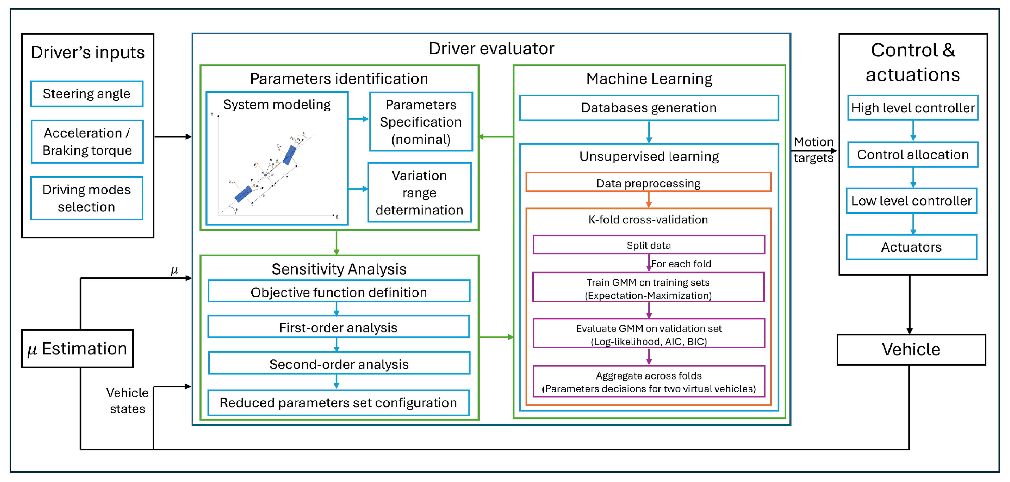
The main contribution of this paper is the preliminary design of the driver evaluator to characterize different driving modes (sport/comfort) using the lateral vehicle dynamics model and physics-assisted machine learning. The proposed algorithm achieves automated parameters set reduction using sensitivity analysis, which significantly improves computational efficiency while maintaining accuracy compared to traditional machine learning methods. Figure 1 presents the overall architecture, including all the detailed steps, which are further clarified in the following sections. The driver inputs the steering wheel angle, torque, and the choice of driving modes into the driver evaluator, which outputs the motion targets to the control system to adjust the car’s performance to be either sporty or comfort. The rest of the paper is organized as follows: a nonlinear bicycle model with Pacejka’s tire model is presented in Section 2 for the case study. The methodology consisting of the mathematical derivation of sensitivity analysis and the unsupervised machine learning is clarified in Section 3. In Section 4, first, the reduced parameters set is obtained from the sensitivity analysis, then the databases are constructed for unsupervised learning. The lateral dynamics of the clustering results are compared between the full parameters set and the reduced one. The conclusion and future work of this paper are stated in Section 5.
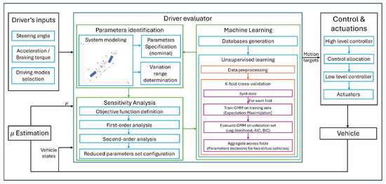
Figure 1.
Overall architecture of vehicle system equipped with a driver evaluator.
2. System Modeling
The bicycle model is the simplest and most used tool to analyze vehicle handling performance. A single-track 2 DOF (Degree Of Freedom) bicycle model is utilized in this study. The effects of the steering system and suspension are neglected. The vehicle which is treated as a rigid body only moves in two dimensional plane with constant longitudinal velocity. A nonlinear Pacejka’s tire model is applied to describe the relationship between slip and tire forces. Moreover, the effects of aerodynamics and lateral load transfer are ignored. The bicycle model with the front wheel angle as input is embedded in Figure 1. The lateral dynamics can be obtained based on Newton’s second law of motion as follows:
where is the lateral tire force. is the lateral acceleration and r is the yaw rate. The remaining parameters are further selected and explained in Table 1.

Table 1.
Bicycle model nominal parameters.
Considering the simplified Pacejka’s tire model, the magic formula is applied to calculate the tire forces as follows:
where is the normal load of front or rear tire. and are the front and rear slip angle, respectively, which can be calculated as:
where u and v are the longitudinal and lateral velocity of the vehicle respectively. In addition, is the front wheel angle as input. B, C, and D are the coefficients of the tire model. represents the cornering stiffness, where B is the stiffness factor, and C is the shape factor that controls the limits of the range of the sine function [15]. The peak factor D is further calculated as follows:
To explore how physical parameters affect vehicle handling performance, the bicycle model is transformed to algebraic equations with parameters as input. The nominal values are given in Table 1, which is a 2019 Jeep Grand Cherokee, obtained from a project in progress [16].
3. Methodology
To distinguish different driving modes regarding the baseline vehicle, a strategy consisting of two key steps is proposed, as illustrated in Figure 1. First, the mathematical interpretation of sensitivity analysis with respect to vehicle physical parameters is introduced to demonstrate their effects on lateral dynamics. Parameters that have little or no influence on the objective function and are not coupled with other high-index parameters can be removed, thereby reducing the number of parameters that need to be taken into account. Secondly, two databases are built for the full and reduced parameters sets, respectively, including the unlabeled lateral dynamics data generated during a specific maneuver. Unsupervised machine learning is then adopted to build a classifier to categorize driving modes based on the driver’s preference. The comparison of the generated motion and understeer gradients between clusters, along with the recorded computational time indicate the strength of this methodology.
3.1. Mathematical Interpretation of Sensitivity Analysis
3.1.1. First-Order Sensitivity Analysis
The first-order sensitivity analysis measures the fractional contribution of each single parameter to the output variance by definition, indicating which parameter has the most influence on the system response [14]. Instead of measuring output changes due to variations in system parameters through simulations, a mathematical description is more straightforward, efficient, and effective.
A factor K is introduced to represent the handling performance of the system, which can be written as an objective function with respect to the vehicle parameters , where The first-order sensitivity index to parameter can be calculated using the Jacobian of the function:
The full set of first-order sensitivities in original unit bases can then be written in a scalar as:
This expression organizes the parameters by their significance. However, it does not illustrate their interactions or couplings with each other. A parameter with a small first-order analysis will affect the system to a small extent, but its strong coupling with other critical parameters is equivalently as important. Therefore, the second-order analysis should be performed.
3.1.2. Second-Order Sensitivity Analysis
The second-order sensitivity analysis measures the interactions between the parameters. This information is very critical regarding which parameters to keep or discard in the final set. Instead of Jacobian, Hessian is applied to generate the following expression:
This yields the correlation sensitivity indices between and . The second-order sensitivity matrix can be written by combining all these indices together:
This expression is useful to keep the parameter that was assumed to be discarded due to its small first-order sensitivity index. The mathematical techniques developed in this section will be utilized with the vehicle model to form the reduced parameters set. It should be emphasized that first-order sensitivity analysis cannot be skipped. For a complex system with numerous parameters, it is difficult to determine which parameters should be checked for coupling with others, by directly applying second-order sensitivity analysis.
3.2. Unsupervised Machine Learning
Given a specific maneuver and different combinations of physical parameters, a large number of cases representing varying virtual models generate unlabeled lateral dynamics data. An unsupervised learning algorithm can be adopted to classify the data into the chosen clusters. It can be categorized as follows: centroid-based, distribution-based, density-based, and hierarchical clustering. It is important to choose the appropriate method for different applications. Since the density-based clustering algorithm automatically determines the number of clusters while the hierarchical clustering algorithm presents the structure of the information rather than the separation of clusters, centroid-based and distribution-based clustering are suitable for this study, as we are mainly interested in the separation of clusters.
This paper adopts a Gaussian mixture model algorithm (GMMs) to classify the driving modes for the proposed bicycle model, accounting for the limited number of vehicle parameters and the possibility of overlapped data distribution. It is a representative distribution-based clustering algorithm. It assumes that all data points are generated from a mixture of a finite number of Gaussian distributions. Unlike K-means which is a typical centroid-based algorithm and the most popular due to its simplicity, the Gaussian mixture model performs soft classification, which provides probabilities of the data points belonging to each of the possible clusters [17]. Rather than assigning data points to the nearest centroids, it fits a set of Gaussian distributions to the data. The probabilities of each data point belonging to each of the clusters can be calculated. Since it performs a soft clustering, the Gaussian mixture model can capture clusters that overlap or have complex boundaries. It is more flexible and able to deal with data that have different sizes and correlation structures. However, it has the same challenges in initialization sensitivity and in guaranteeing convergence to the global optimal as K-means.
To ensure robustness and reliability, k-fold cross-validation is applied to ensure that it generalizes well to different data subsets and accurately captures the underlying structure of the data. The database is randomly partitioned into k folds of equal size. Each fold is retained as the validation data, and the remaining k-1 folds are treated as training data. Then, a GMM is fitted to the training sets and evaluated on the validation set. After repeating the cross-validation process k times, the separate and average performance scores over all folds can be calculated [18]. The integration of log-likelihood, AIC (AKaike Information Criterion), and BIC (Bayesian Information Criterion) offers a robust methodology for evaluating GMMs. Log-likelihood quantifies the probability of the observed data under the model, with higher values indicating a better fit [19]. However, simply maximizing the log-likelihood can result in overfitting, which poses necessity in using AIC and BIC to penalize model complexity [20]. AIC estimates the relative amount of information lost when a given model is used to represent the process that generates the data, while BIC is another criterion with a stronger penalty for complex models [21]. Lower AIC and BIC values indicate a better trade-off between model fit and complexity. When measuring the performance of GMMs, log-likelihood provides a direct measure of the model’s fit to the data, which is then adjusted by AIC and BIC to account for model complexity [22].
4. Results and Discussion
In this section, following the steps outlined in Figure 1, the objective function is built to analyze the handling performance of the bicycle model. The first-order sensitivity analysis is performed to find the parameters which have little or no influence on the lateral dynamics. To further investigate the impact of the parameters that should have been ignored according to their low first-order sensitivity index, the second-order analysis is then performed to explore the correlation between the parameters. In the final subsection, a step-steer test is conducted for all cases to establish the database of the reduced parameters set and original full set, respectively. Comparisons of motion and understeer gradients between the GMM clustering results help to specify the driving modes and validate the key role of the sensitivity analysis.
4.1. Sensitivity Analysis Results
4.1.1. First-Order Sensitivity Analysis Results
In a bicycle model, the lateral acceleration and yaw rate are the key responses that reflect its handling performance, which can be represented as metric K as follows:
where and are the contribution factors, determined by the priority of maneuverability and stability. In this paper, only lateral acceleration is taken into account because we do not focus on stability, assigning and . The analysis of K can then be calculated as the normalized sensitivity of , considering different scales and units of the various parameters. In addition, the absolute value of the changes is applied.
Instead of considering the effects of a and b separately, L is introduced as the sum of a and b, which remains constant. Changes in a indicate the shift of the CG position forward or aft. The nominal values of the physical parameters are determined from the baseline vehicle in Table 1. Since the tire model used in the Jeep [16] is “SUV 265/50R20”, the tire parameters can be estimated as and . The value of the stiffness factor B can be calculated by dividing the cornering stiffness by . The full parameters set can be written as . Three cases using the same step steer angle input but different initial longitudinal velocities are conducted in Matlab/Simulink on the nonlinear bicycle model built in the previous section, resulting in steady-state lateral accelerations of approximately , , and , respectively. The first-order sensitivity indices can be calculated with respect to the full parameters set as:
where represents the normalized sensitivity index of at an initial longitudinal velocity of 10 m/s, at 20 m/s, and at 30 m/s. In more detail, for , 0.0393 is the index with respect to m, while 0.7457 is relative to a. These three equations follow a trend that is consistent with the characteristics of the nonlinear Pacejka’s tire model. The tire parameters have a significant impact on the vehicle’s handling performance in the linear region, where the slip angle is small. However, due to tire force saturation, their influence diminishes in the nonlinear region.
It is no surprise that the greatest first-order sensitivity scalar is related to a, which reveals the most significant parameter for vehicle handling performance, and is consistent between these three cases, while has little or no influence. Increasing a, which means shifting the CG position backward, will significantly change the lateral dynamics. The parameters , B and C which are related to the cornering stiffness also have great effects on vehicle handling performance, compared to m, , and . The results are consistent with the conclusion from [23], where Salem found that the most significant changes occur as a result of moving vehicle CG position and thereby altering its understeer or oversteer balance by manually tuning each parameter within a ten percent deviation and checking the lateral acceleration response on a linear bicycle model. Moreover, from the first-order sensitivity analysis, can be removed from the parameters set utilized for the machine learning, but further investigation about m and is required due to its moderate first-order sensitivity value.
4.1.2. Second-Order Sensitivity Analysis Results
To further simplify the features of machine learning and verify the feasibility of the results of the first-order sensitivity analysis, a second-order analysis is performed to measure the correlation between m and with the other four parameters, , B, C and a. Since the matrix is symmetric, and only off-diagonal values represent the interactions. The 7 × 7 matrix could be simplified and derived from the vehicle seven parameters, using the upper triangular matrix without the diagonal values. The same nominal values used in the first-order sensitivity analysis are applied, and the results are presented in the following matrix:
The ith row illustrates the coupling of the ith parameter with itself and the other parameters. Therefore, the large values of , and illustrate the strong coupling of the fourth, fifth, and sixth parameters with the seventh parameter. This indicates that tire parameters , B, and C are strongly coupled with the distance from the CG to the front axle. These four parameters form the reduced set, expressed as , which is delivered to the machine learning block. In addition, the small values in the first three rows reveal minor or no coupling between m, , and with the other four parameters, justifying their removal for the subsequent set. Only the results for case 1 are presented here, as the second-order sensitivity analysis leads to the same conclusion regarding the establishment of the reduced set.
The results demonstrate the significance of the second-order sensitivity analysis. The parameters that have no impact on the handling performance from the first-order analysis need to be verified to have no coupling with the other critical parameters. This reduced set will be fed into unsupervised learning to classify the driving modes.
4.2. Machine Learning Simulation Results
4.2.1. Database Construction with Step-Steer Test
To identify the different driving modes, it is important to understand their definition and the key difference. Generally, as aforementioned, comfort mode provides softer suspension, slower throttle and gearbox responses, and lighter steering [24]. This mode is suitable for those who prefer a gentle driving experience for the daily commute. In contrast, the sport mode is designed for enthusiastic drivers with increased responsiveness from the engine, and the gearbox. Žuraulis [24] only considers the longitudinal vehicle dynamics and its impact on these modes. In contrast, this paper only considers the lateral vehicle dynamics and their impact. In this analysis, the sport mode is considered to have a consistently reduced understeer gradient and an increased maximum value of lateral acceleration and yaw rate for a given wheel angle and initial speed compared with the comfort mode [3]. Higher lateral accelerations are observed for the sport mode compared to the comfort mode when the speed is above 40 km/h. Additionally, the yaw rate difference is especially visible for speeds above 55 km/h [2]. A good starting point for the simulation setup is then obtained from these speed ranges.
Two databases are created for the nonlinear bicycle model considering the full and the reduced parameters set, respectively. The range for each parameter is assumed to be from the baseline vehicle, with the values determined by the capacity threshold of active actuator sets. The detailed parameters for Pacejka’s tire model can be estimated based on SUV 265/50R20 tire model in Simulink from the baseline vehicle. These ranges are divided into three equal intervals for each parameter. By assigning different values to the front and rear tire parameters, and randomly combining all parameters together, cases are established for data generation. The step-steer test is then conducted in Simulink after dropping all oversteer cases to generate the system responses for each case. According to the ISO standard 7401 [25], a fast tire wheel input of 1.5 degrees with an initial vehicle speed of 20 m/s is applied. The simulation results for each case are merged into a database for the machine learning algorithm.
4.2.2. Gaussian Mixture Models Clustering Results
After loading all the data points, normalization is first performed to reduce large-scale differences. A Gaussian mixture model is then fitted to the data after initialization. A 5-fold cross-validation is then applied to assess the model’s performance through evaluating the log-likelihood, AIC (Akaike Information Criterion), and BIC (Bayesian Information Criterion). After comparing these three metrics across five subsets, the two centroids from the fold with lowest AIC and BIC, as well as relative higher log-likelihood values are chosen to represent the clustered sport and comfort vehicle, respectively. The corresponding parameter values are listed in Table 2, where cornering stiffness is presented instead of the tire parameters. The parameters excluded based on the sensitivity analysis results are set to be consistent with those of the baseline vehicle. All units are consistent with Table 1.

Table 2.
Parameters of the sport and comfort vehicle models from the clustering results.
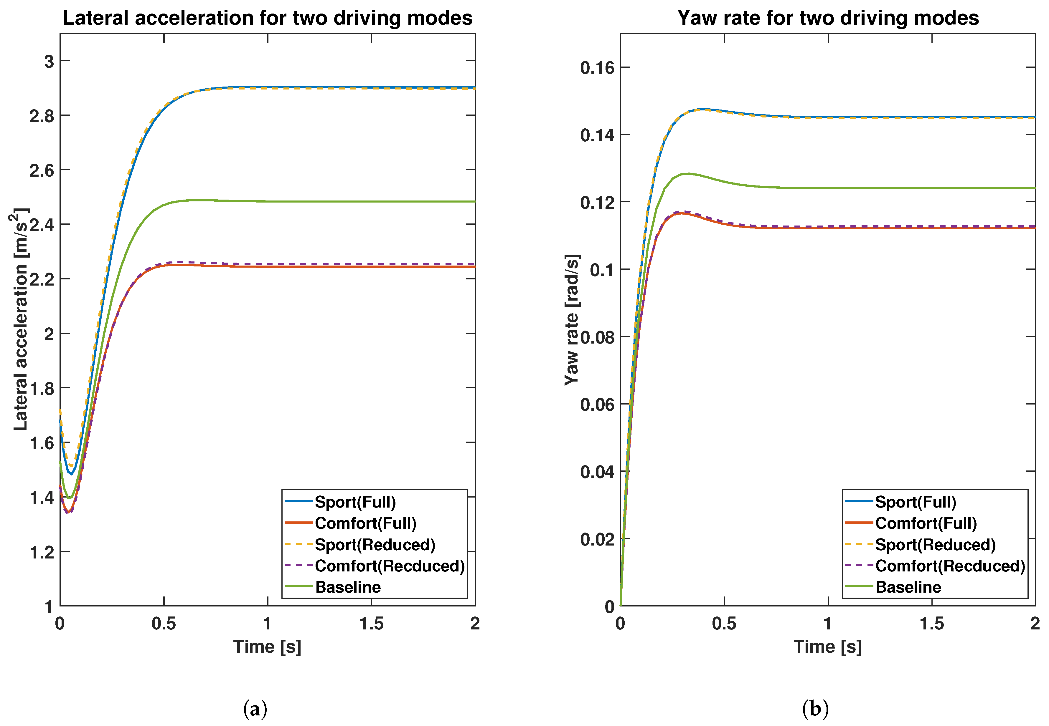
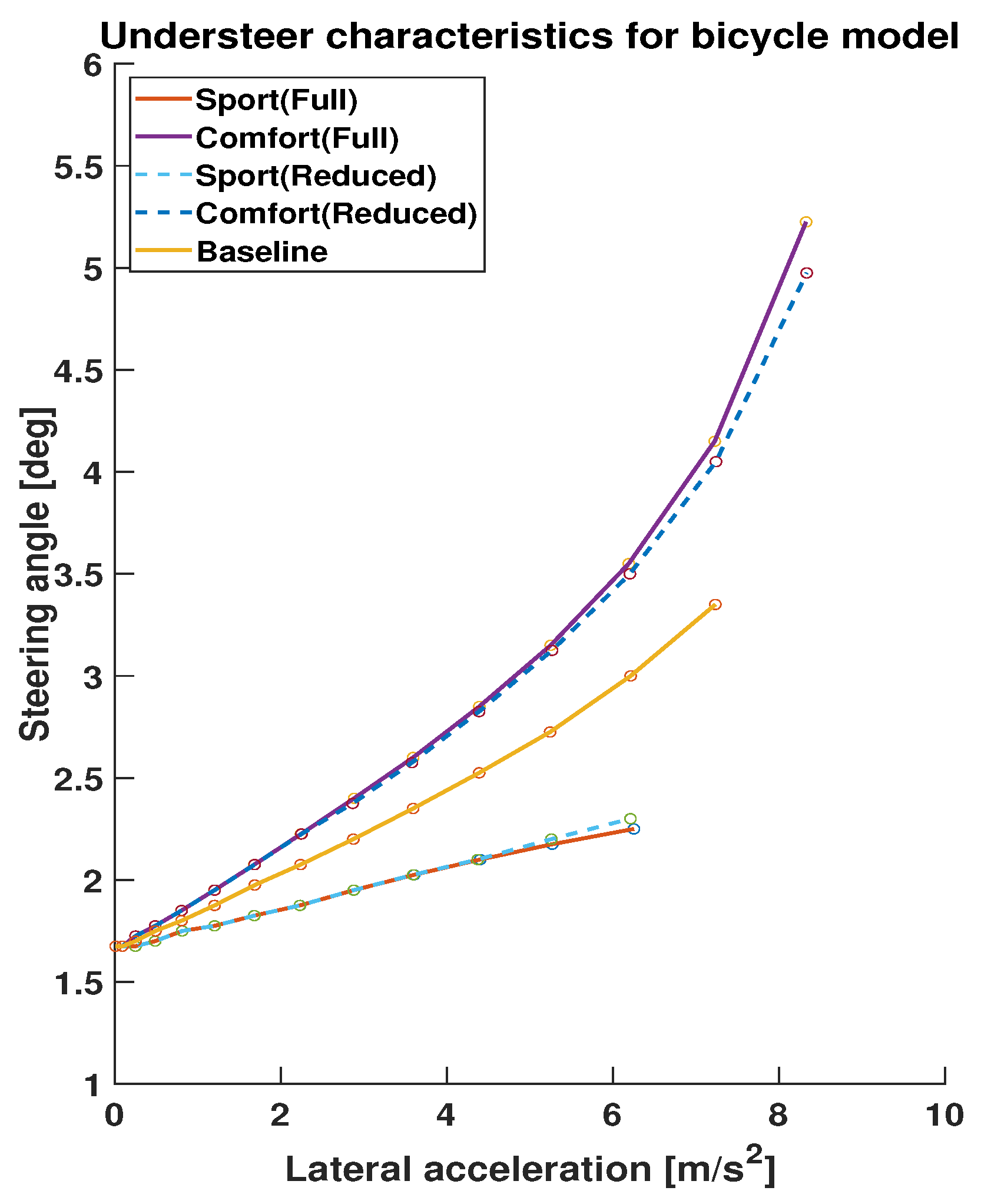
To further visualize the clustering results, two tests are conducted on the vehicles built using the parameters from the two centroids for both the full and reduced parameters sets. First, a step-steer test is performed with an initial longitudinal speed of 20 m/s, and a 1.5-degree wheel angle. Secondly, a constant radius test is applied with a test radius of 100 m. During the test, the longitudinal speed is gradually increased, and the steering angle is simultaneously adjusted to make the vehicle follow a circular trajectory with the given radius. The plot of steering angle input versus lateral acceleration illustrates the understeer characteristics, which is a key metric influencing the vehicle’s handling performance. Figure 2 shows the comparison results of lateral acceleration and yaw rate, respectively, between the two databases and the baseline vehicle. In addition, Figure 3 shows the comparison results of the understeer characteristics.
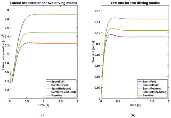
Figure 2.
(a) Lateral acceleration comparison results between two databases and baseline vehicles. (b) Yaw rate comparison results between two databases.
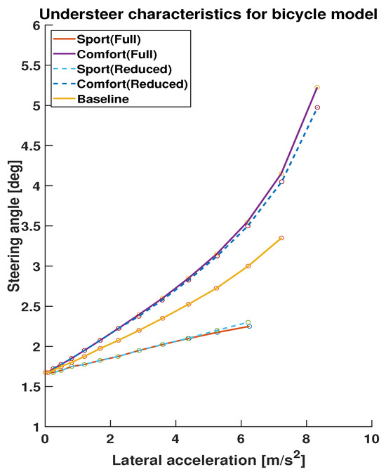
Figure 3.
Understeer characteristics comparison results between two databases and baseline vehicles.
A very small difference is observed in the lateral dynamics as well as the understeer characteristics for the two databases built using the full and reduced parameters sets, which demonstrates the accuracy of the physics-assisted machine learning. The small deviation in the nonlinear region is acceptable. Furthermore, simulation times are recorded and compared to highlight the improvement in computational efficiency. The simulation for the database with the full parameter set takes 20.79 s, but it is only 0.30 s for the database with the reduced set. There is no doubt that it will be more beneficial for higher-fidelity models with a large number of parameters. Therefore, the simulation results verify the feasibility and applicability of the sensitivity analysis in obtaining reduced parameter sets for machine learning applications. The accuracy of machine learning is maintained while computational efficiency is improved by reducing the size of the database.
5. Conclusions
This paper proposes a sensitivity analysis-based machine learning strategy that can acquire different driving modes with reduced computational overhead. The 2DOF bicycle model with nonlinear Pacejka’s tire model is utilized to generate lateral motions for specific maneuvers. The results of the first-order sensitivity analysis suggest the removal of (moment of inertia) from the parameters set and further investigation for the removal of m (mass) and (tire parameter) is proposed. Then, the second-order sensitivity analysis confirms their removal and determines the reduced parameters set. The Gaussian mixture models cluster the simulation data from the step-steer maneuver into sport and comfort modes. K-fold cross-validation and the consideration of log-likelihood, AIC, and BIC metrics are integrated to assess the GMMs. Comparing the lateral dynamics from the database with the full parameters set, the proposed method illustrates great accuracy for driving modes classification with high computational efficiency. This work has great significance and practical implications for higher degrees of freedom systems with large datasets. In the future, we will investigate our proposed approach with a 7DOF vehicle model and a full vehicle model with a suspension system while combining the longitudinal and lateral motions, as well as the four-wheel rotational motions. In addition, sensor data will be collected to fine-tune and adapt the virtual models. Furthermore, this driver evaluator has great potential for future investigation of combing the current work with the optimization technique for trajectory generation for application of collision avoidance.
Author Contributions
Conceptualization, M.H.; methodology, M.H.; software, M.H.; validation, M.H.; formal analysis, M.H.; investigation, M.H.; resources, M.H.; data curation, M.H.; writing—original draft preparation, M.H.; writing—review and editing, M.H. and F.A.; visualization, M.H.; supervision, F.A. All authors have read and agreed to the published version of the manuscript.
Funding
This research received no external funding.
Institutional Review Board Statement
Not applicable.
Informed Consent Statement
Not applicable.
Data Availability Statement
The original contributions presented in this study are included in the article. Further inquiries can be directed to the corresponding author(s).
Conflicts of Interest
The authors declare no conflicts of interest.
References
- Sheller, M. Automotive emotions: Feeling the car. Theory Cult. Soc. 2004, 21, 221–224. [Google Scholar] [CrossRef]
- Melman, T.; Winter, J.D.; Mouton, X.; Tapus, A.; Abbink, D. How do driving modes affect the vehicle’s dynamic behaviour? Comparing Renault’s Mult-Sense sport and comfort modes during on-road naturalistic driving. Veh. Syst. Dyn. 2021, 4, 485–503. [Google Scholar] [CrossRef]
- Novellis, L.D.; Sorniotti, A.; Gruber, P. Driving modes for designing the cornering response of fully electric vehicles with multiple motors. Mech. Syst. Signal Process. 2015, 64–65, 1–15. [Google Scholar] [CrossRef]
- Kim, Y.; Choi, S.B.; Oh, J.J.; Eo, J. Satisfactory Driving Mode Classification Based on Pedal Operation Characteristics. IEEE Trans. Intell. Veh. 2024, 9, 2988–2998. [Google Scholar] [CrossRef]
- Eftekhari, H.R.; Ghatee, M. A similarity-based neuro-fuzzy modeling for driving behavior recognition applying fusion of smartphone sensors. J. Intell. Transp. Syst. 2019, 23, 72–83. [Google Scholar] [CrossRef]
- Lin, N.; Zong, C.; Tomizuka, M.; Song, P.; Zhang, Z.; Li, G. An overview on study of identification of driver behavior characteristics for automotive control. Hindawi Publ. Corp. Math. Probl. Eng. 2014, 2014, 569109. [Google Scholar] [CrossRef]
- Sutton, R.S.; Barto, A.G. Reinforcement Learning: An Introduction, 2nd ed.; The MIT Press: Cambridge, MA, USA; London, UK, 2018. [Google Scholar]
- Hao, Z.; Liu, S.; Zhang, Y.; Ying, C.; Feng, Y.; Su, H.; Zhu, J. Physics-informed machine learning: A survey on problems, methods and applications. arXiv 2023, arXiv:2211.08064. [Google Scholar]
- Koysuren, K.; Keles, A.F.; Cakmakci, M. Online Parameter Estimation using Physics-Informed Deep Learning for Vehicle Stability Algorithms. In Proceedings of the 2023 American Control Conference (ACC), San Diego, CA, USA, 31 May–2 June 2023; pp. 466–471. [Google Scholar]
- Liu, J.; Han, X.; Pan, Y. Physics-assisted machine learning methods for predicting the splitting tensile strength of recycled aggregate concrete. Sci. Rep. 2023, 13, 9078. [Google Scholar] [CrossRef] [PubMed]
- Othaganont, P.; Assadian, F.; Auger, D. Sensitivity analyses for cross-coupled parameters in automotive powertrain optimization. Energies 2014, 7, 3733–3747. [Google Scholar] [CrossRef]
- Mantripragada, V.K.T.; Kumar, R.K. Sensitivity analysis of tyre characteristic parameters on ABS performance. Veh. Syst. Dyn. 2022, 60, 47–72. [Google Scholar] [CrossRef]
- Suarez, B.; Felez, J.; Maroto, J.; Rodriguez, P. Sensitivity analysis to assess the influence of the inertial properties of railway vehicle bodies on the vehicle’s dynamic behaviour. Veh. Syst. Dyn. 2012, 51, 251–279. [Google Scholar] [CrossRef]
- Hassan, M.A.; Abdelkareem, M.A.; Tan, G.; Moheyeldein, M.M. A Monte Carlo parametric sensitivity analysis of automobile handling, comfort, and stability. Hindawi Shock Vib. 2021, 2021, 6638965. [Google Scholar] [CrossRef]
- Pacejka, H.B. Tyre and Vehicle Dynamcis, 2nd ed.; Elsevier/BH: Amsterdam, The Netherlands, 2006. [Google Scholar]
- Langari, R. AVA: Automated Vehicles for All. U.S. Department of Transportation. Available online: https://rip.trb.org/View/1878930 (accessed on 20 April 2023).
- Pevneva, A.G.; Inna, P. Comparison of the probabilistic model of a fuzzy Bayesian classifier and the Gaussian mixture problem. J. Phys. Conf. Ser. 2022, 2373, 062022. [Google Scholar] [CrossRef]
- Buffle, E.; Papadis, A.; Blaser, I.; Nozica, N.; Kassar, M.; Ludwig, R.; Berger, D.; Haenggi, M. In-vivo validation of a nomogram with isostiffness-lines for the assessment of aortic stenosis severity. Eur. Heart J. 2023, 44, ehad655.033. [Google Scholar] [CrossRef]
- Prusti, D.; Behera, R.K.; Rath, S.K. Hybridizing graph-based Gaussian mixture model with machine learning for classification of fraudulent transactions. Comput. Intell. 2022, 38, 2134–2160. [Google Scholar] [CrossRef]
- Liu, H.; Roeder, K.; Wasserman, L.A. Stability Approach to Regularization Selection (StARS) for High Dimensional Graphical Models. Adv. Neural Inf. Process. Syst. 2010, 24, 1432–1440. [Google Scholar] [PubMed]
- Vrieze, S.I. Model selection and psychological theory: A discussion of the differences between the akaike information criterion (aic) and the bayesian information criterion (bic). Psychol. Methods 2012, 17, 228–243. [Google Scholar] [CrossRef] [PubMed]
- Dziak, J.J.; Coffman, D.L.; Lanza, S.T.; Li, R.; Jermiin, L.S. Sensitivity and specificity of information criteria. Brief. Bioinform. 2019, 21, 553–565. [Google Scholar] [CrossRef] [PubMed]
- Salem, M.M.M.; Ibrahim, M.M.; Mourad, M.A.; EI-Gwwad, K.A.A. Sensitivity analysis of vehicle parameters on dynamic stability and vehicle handling performance. Int. J. Veh. Struct. Syst. 2021, 13, 65–71. [Google Scholar] [CrossRef]
- Žuraulis, Ž.; Robertas, P.; Mourad, M.A.; Ginas, J. Semi-Active Suspension Influence on Comfort Sensation of a Vehicle Occupant. Available online: https://api.semanticscholar.org/CorpusID:55490476 (accessed on 15 March 2022).
- ISO 7401; Road Vehicles: Lateral Transient Response Test Methods = Véhicules Routiers: Méthodes d’Essai en réGime Transitoire sous AccéLération latéRALE, 1st ed. International Organization for Standardization: Geneva, Switzerland, 1988.
Disclaimer/Publisher’s Note: The statements, opinions and data contained in all publications are solely those of the individual author(s) and contributor(s) and not of MDPI and/or the editor(s). MDPI and/or the editor(s) disclaim responsibility for any injury to people or property resulting from any ideas, methods, instructions or products referred to in the content. |
© 2025 by the authors. Licensee MDPI, Basel, Switzerland. This article is an open access article distributed under the terms and conditions of the Creative Commons Attribution (CC BY) license (https://creativecommons.org/licenses/by/4.0/).

