Abstract
The Xfinity Racing Series is an American stock car racing series organized by NASCAR. For the 2017 racing season, NASCAR introduced new regulations with the objective of creating a level playing field by reducing aerodynamic influence on vehicle performance. In this context, the primary objective of this work is to explore the differences in the aerodynamic performance between the 2016 and 2017 Toyota Camry Xfinity racecars using only open-source Computational Fluid Dynamics (CFD) and CAE tools. During the CFD validation process, it was observed that none of the standard turbulence models, with default turbulence model closure coefficients, were able to provide racecar aerodynamic characteristics predictions with acceptable accuracy compared to experiments. This necessitated a fine-tuning of the closure coefficient numeric values. This work also demonstrates that it is possible to generate CFD predictions that are highly correlated with experimental measurements by modifying the closure coefficients of the standard SST turbulence model.
1. Introduction
Stock car racing is truly an American phenomenon. This is a form of automobile racing in which cars that conform externally to standard U.S. commercial types are raced, usually on oval, paved tracks. Stock car racing is said to have originated during the U.S. Prohibition period (1919–1933), when illegal still operators, needing private cars capable of more than ordinary speed to evade the law while transporting liquor, tuned and altered ordinary passenger automobiles to make them faster [1]. Subsequently, these cars were raced for pleasure, particularly in the southeastern states, where the sport remained most popular. Organized stock car racing began at Langhorne, Pennsylvania, in 1939. The National Association for Stock Car Auto Racing (NASCAR), founded in 1947 at Daytona Beach, Florida, gave the sport its first formal organization. The sport had become popular on the beach at Daytona Beach from the 1930s, but the first organized racing in Daytona took place in 1948. By the 1970s, several other organizations, including the United States Auto Club (USAC), also sponsored stock car races [1]. Over the years, as a racing sanctioning body, NASCAR has evolved as the American equivalent of the Fédération Internationale de l’Automobile, commonly referred to as the FIA, which regulates the world’s most prestigious motorsports, Formula 1 or F1. It is needless to say that NASCAR has positioned itself as one of the world’s premier motorsports organizations, and NASCAR races are among the most-watched sporting events in the United States.
According to its website (https://www.nascar.com/; accessed on 30 July 2024), NASCAR currently serves as the Sectioning Body for five race series: the Cup Series, Xfinity Series, Truck Series, International Series, and Roots Series. Of these series, the first three are known as the Stock Car Racing Series, in which three major Automotive Original Equipment Manufacturers (or OEMs), General Motors (GM), Ford, and Toyota, participate. Among the three stock car racing series sanctioned by NASCAR, the Cup Series is regarded as by far the most coveted one, followed by the Xfinity and Pick-up Truck Series. The Xfinity Series is primarily dominated by the OEM-supported Cup Series teams, although there are several minor non-Cup teams competing in the Series, in which the Cup teams aim to provide their young drivers with experience in longer races (180–300 miles) during a season that includes many companion races to Cup Series events. While some Xfinity Series teams remain family-owned or independent, most of the season’s races are won by cars and drivers connected to Cup Series operations and major automakers. These lower-series cars are slightly less powerful than Cup cars but provide valuable practice for drivers, including some Cup drivers who compete in these divisions for extra track time and winnings, and serve as a proving ground for future Cup Series stars but also feature a mix of young talents, veterans returning from unsuccessful Cup careers, independent owners/drivers, and occasional appearances by Cup regulars. A reader interested in these non-engineering aspects of NASCAR races is directed to the thesis of Swansey [2].
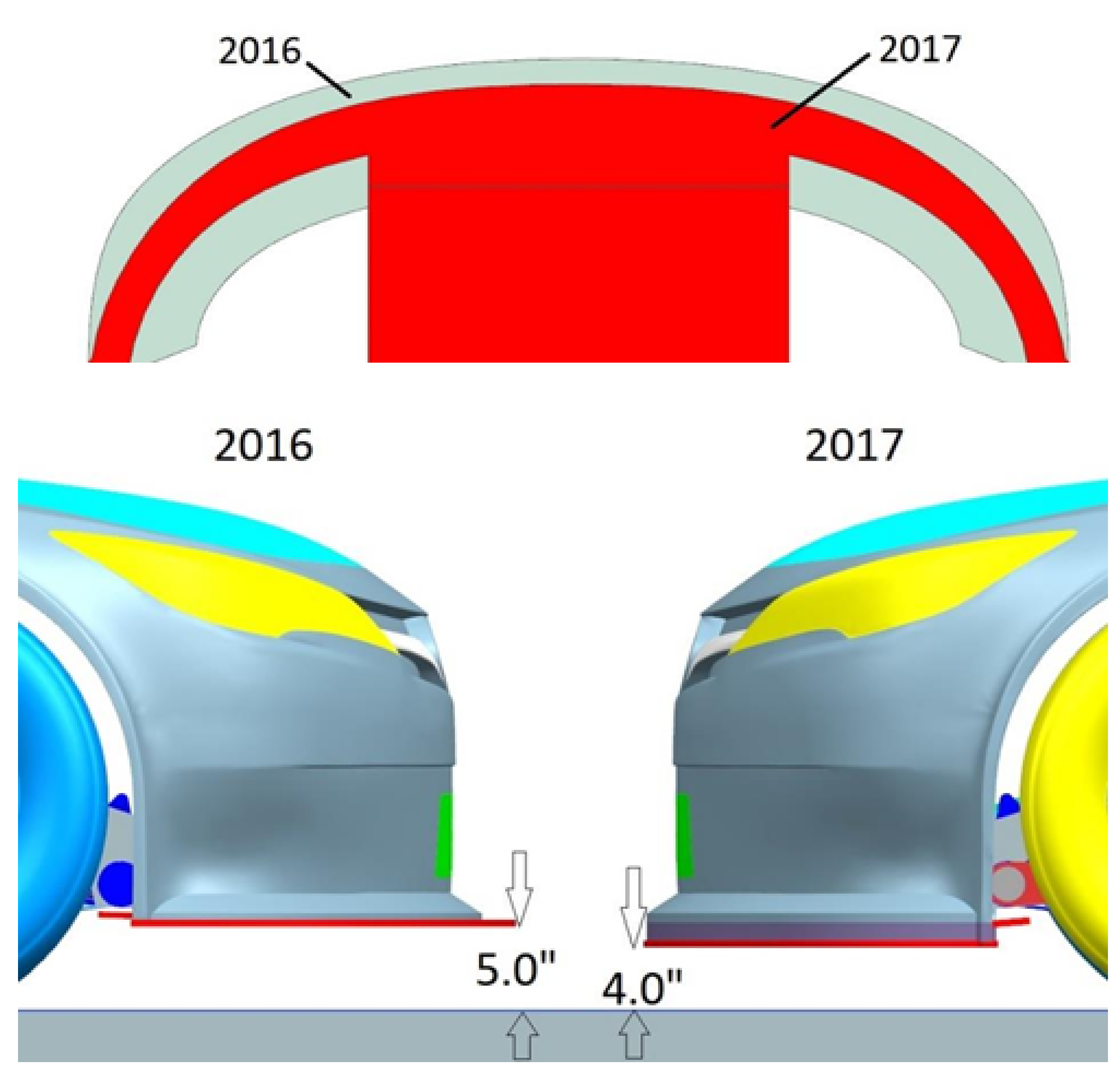
At the beginning of the 2017 season, NASCAR implemented significant aerodynamic rule changes for both the Monster Energy NASCAR Cup Series and the Xfinity Series. The primary goal was to diminish aerodynamic forces and enhance the overall quality of racing. This significant alteration shifted the emphasis away from relying solely on vehicle performance to placing a greater premium on the skills of the drivers. One notable change involved the reduction in spoiler height, a deliberate move intended to decrease rear down-force and minimize the vehicle drag. Spoiler shape was changed and the width was also reduced to protect the spoiler in the event of hitting a wall on the race track. Finally, spoiler ears were eliminated for the 2017 race season. Figure 1 shows 2016 and 2017 Toyota Camry Xfinity Series racecars. An overlay of 2016 and 2017 spoilers is also shown in Figure 1 (Bottom), giving a good visual comparison of these two spoiler configurations. As we also can see in Figure 1, the other change for 2017 involved reducing the area of the racecar’s front splitter plate. To maintain the car’s aerodynamic balance, front down-force was reduced by making the front splitter 162.4 mm (6 inches) shorter on the sides and 50.8 mm (2 inches) shorter in the center. Figure 2 illustrates the distinctions between the splitter configurations used in the 2016 and 2017 seasons. This comparison encompasses not only the changes in the splitter dimensions but also a reduction in the ground-to-splitter-bottom clearance, referred to as the splitter-gap. The splitter-gap was reduced from 127 mm (5 inches) to 101.6 mm (4 inches), which is slated to facilitate an easier inspection process.
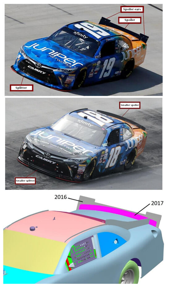
Figure 1.
Toyota Xfinity Series racecars. (Top): 2016 car; (Middle): 2017 car; (Bottom): 2016 and 2017 rear spoiler differences.

Figure 2.
Comparison of the 2016 and 2017 season splitter configurations, with the 2017 configurations highlighted in red. The 2017 car features a smaller splitter surface (Top) and a lower splitter gap (Bottom) compared to the 2016 model.
We became interested in understanding the extent to which these changes would impact the on-track aerodynamic performance of the Xfinity racecars. While wind tunnel tests could have provided a straightforward answer regarding the implications for drag, down-force (negative lift), and front balance (the ratio of front down-force to total down-force), they are prohibitively expensive. Moreover, wind tunnel tests do not offer detailed quantitative knowledge about the effects of these changes on the overall flow field around the car, which is one of our major interests. In this regard, Computational Fluid Dynamics (CFD) appears to be the most optimal tool, and has long been used to comprehend the effects of geometry changes on the overall drag of a car, including the underhood flow [3].
While the literature is abundant with CFD studies investigating various aspects of passenger vehicles, research on stock racecars, especially involving Xfinity racecars, is limited. The majority of NASCAR Cup racecar aerodynamics-related work has been conducted by Uddin and his colleagues at the University of North Carolina, Charlotte [4,5,6,7,8]. These studies explored the impact of solver parameters, boundary conditions, and turbulence modeling on the effectiveness of CFD predictions, utilizing the commercial CFD code Star-CCM+ by Siemens. On the other hand, investigations related to Xfinity Series racecars are primarily attributed to Jacuzzi and colleagues (cf. [9,10]), who examined passive flow control for drag reduction in vehicle platoons. Specifically, they explored how blowing could influence the vehicle wake. Another noteworthy contribution in Xfinity Series cars comes from Catranis [11], who aimed to improve the accuracy of steady-state Reynolds-Averaged Navier–Stokes (RANS) CFD simulation by systematically adjusting refinement parameters within the simulation mesh settings. These simulations were conducted using OpenFOAM with two NASCAR Xfinity Series vehicles and were validated against wind tunnel data.
Commercial CFD codes, such as Siemens Star-CCM+, Anysys Fluent, or Dassault Systèmes PowerFLOW, are very expensive. Therefore, an additional goal of the work presented here is to establish a high-fidelity CFD simulation framework utilizing open-source codes, aiming to mitigate the costs associated with CFD simulations.
The work presented in this paper originated from the Master’s thesis work of Nazarii Olkhovskyi [12] at the University of North Carolina, Charlotte. As mentioned in the Acknowledgment section as well, the racecar model and all wind tunnel test data for the project were provided by the sponsor of the project, Joe Gibbs Racing, 663 Huntersville, NC, 28078, U.S.A.
2. Methodology
As mentioned earlier, this study involved a comparison between the 2016 and 2017 aerodynamic devices at various vehicle attitudes. An extensive Computational Fluid Dynamics (CFD) analysis was conducted to investigate the aerodynamic effects on vehicle forces, and it delves into investigating changes in airflow around the car and how they impact both local and global forces acting on the vehicle.
To accomplish this in CFD, a comprehensive ride height model that accounts for the vehicle suspension’s kinematics had to be developed. When the car changes its ride height, all vehicle components shift their positions relative to the wind tunnel. Given that an assembly comprises over a hundred parts, regenerating and exporting CAD models for each part posed a substantial task. To streamline this process, a decision was made to fix all sprung vehicle components and move the wind tunnel and all unsprung components with respect to it. This reduces the number of parts requiring export to only the suspension components and wind tunnel boundaries. Rather than moving the car concerning the wind tunnel, it was decided to move the wind tunnel concerning the car.
Siemens NX CAD software was utilized for the development of all 3D models and their subsequent export for CFD simulations. OpenFOAM, an open-source software package, was employed for CFD simulations, comprising the SnappyHex mesher, OpenFOAM solvers, and ParaView post-processing tools. The mesher subdivides the volume around the car in a virtual wind tunnel into hexahedral cells, with the solver employing this mesh to calculate and transfer flow properties between cells. The post-processing tool aids in data visualization and the generation of plots and figures. The results were compared to flow visualization data from the wind tunnel, and global drag, down-force, and side-force were contrasted with coefficients obtained during wind tunnel tests for both the 2016 and 2017 aerodynamic packages.
The utilization of open-source software introduced additional challenges. Not many open-source meshers can generate hexahedral or polyhedral meshes exceeding 120 million cells, and they must support parallel processing while producing boundary layers with specified thickness. SnappyHexMesh was selected based on these requirements. Although it lacks a graphical interface, users can modify dictionary files and create user-defined scripts to generate custom meshes.
OpenFOAM has gained popularity as an open-source CFD software comparable to commercial counterparts over the past decade. It offers a wide range of solvers for different simulation types. ParaView, a data visualization software, was employed for post-processing and is available to the public at no cost. Similar to SnappyHexMesh and OpenFOAM, it is customizable and allows for the development of custom scripts to automate post-processing.
A last note on the methodology: The 2017 rule change lowered the splitter by 1 inch, resulting in a higher vehicle body position compared to the 2016 rule package at the same splitter heights. Given the dominant influence of splitter height on aerodynamic performance, the decision was made to compare the two aerodynamic packages at common splitter-gaps rather than common body positions.
3. Governing Equations
OpenFoam solves the Navier–Stokes equations which govern the flow field around any object. These equations mathematically express the principles of Conservation of Mass, commonly known as the Continuity Equation, and the Conservation of Momentum, as expressed through Equations (1) and (2), respectively, utilizing Einstein notation. In this notation, repeating index variables (e.g., i or j) imply summation over all possible values (i.e., ).
In these equations, t and represent time and the spatial coordinate in the i direction, respectively, while variables u, p, , T, e, K, and denote the time-dependent values of the velocity, pressure, fluid density, temperature, internal energy, thermal conductivity, and fluid viscous stress tensor, respectively. With as the fluid kinematic viscosity and as the instantaneous rate of the strain tensor, the viscous stress tensor, , is defined as
The instantaneous rate of the strain tensor is defined as
A Direct Numerical Simulation (DNS) of the Navier–Stokes equations requires resolving the flow to the smallest time and length scales, which is impossible to carry out even with the most powerful computer on earth. This makes the Reynolds-Averaged Navier–Stokes (RANS) approach the commonly used method for CFD solutions of engineering problems. This approach is based on Reynolds decomposition, which decomposes an instantaneous quantity into mean and fluctuating components. If the lower- and upper-case symbols denote the instantaneous (or time-dependent) and average values, respectively, and the primed variable means the fluctuating component, then this can be expressed mathematically as . Thus, with this convention, , , and represent the time-dependent instantaneous, time-averaged, and time-dependent fluctuating parts of the velocity component in the i direction, respectively.
Six additional terms in the form of are introduced into the system of equations as a consequence of the Reynolds averaging process, which brings the number of independent variables to 10, while the system only has four equations. This is known as the closure problem in fluid dynamics, which is often resolved using the turbulent viscosity hypothesis introduced by Boussinesq in 1877. Per Boussinesq’s hypothesis, a connection is required between turbulent stresses and the mean rate of strain, analogous to the viscous stress relationship given in Equation (3). However, in this scenario, the constant of proportionality takes the form of a fictitious flow variable known as the “turbulent eddy viscosity”, denoted as in Equation (7).
Here, k is the turbulence kinetic energy per unit mass, , and is the Kronecker delta. The determination constitutes the focal point of turbulence modeling approaches. Eddy viscosity-based turbulence models available in the literature primarily diverge in how they estimate and what other constitutive relationship or transport equations are used in order to derive . Modern turbulence modeling methods typically involve solving additional transport equations to determine . These modeling approaches are categorized based on the number of transport equations and the specific transport variables used in the modeled equations. For instance, a one-equation turbulence model entails solving a single additional transport equation, while a two-equation approach like the modeling approach requires the transport of turbulence kinetic energy and a specific rate of turbulence kinetic energy dissipation .
The current study uses the SST , referred to as simply SST in discussions to follow. The SST model was originally proposed by Menter and subsequently further improved by his coworkers [13,14]. Though a short description is provided below, the interested reader is referred to Zhang et al. [15] and the original articles of Menter and coworkers [13,14,16] for a more comprehensive read.
Shear Stress Transport (SST) Turbulence Model
The SST is a hybrid model that takes the advantage of Wilcox’s standard model [17,18] in the near-wall region while also retaining the strength of the model of Launder and coworkers (see [19,20]) in the far-field freestream region. In addition, this model includes an additional non-conservative cross-diffusion term containing in the transport equation. This cross-diffusion term is used only in regions far from the wall by using a blending function. The expressions for the eddy viscosity and the transport equations are given in Equations (8)–(15).
where , and are the closure coefficients of the model. The values of these coefficients are computed using blending functions and the corresponding constants of the and models via the relationships , etc.
4. Geometry, Mesh, and Solver Settings
A Toyota Camry NASCAR Xfinity Series racecar, as used by the sponsor of the project, Joe Gibbs Racing, was selected for the simulation. This model, introduced in 2015, remained in use until the conclusion of 2018, when it was succeeded by the Toyota Supra NASCAR Xfinity Series racecar (please see Figure 1). This study required the creation of a three-dimensional CAD model exhibiting a true representation of the car. Ensuring an accurate representation of the vehicle involves a meticulous process. For this purpose, the whole body and all external components for which CAD data did not exist were scanned using a white light scanner generating a point cloud within 0.002 inches of the actual surface. This point cloud underwent a cleaning process to eliminate unwanted data, followed by surfacing and thickening to produce a clean, closed volume ideal for CFD simulations. Subsequent to this, achieving the exact same attitude of the vehicle in the wind tunnel is of utmost importance. To accomplish this, a kinematic ride height model was developed. This model utilizes the splitter-to-ground distance to establish the front ride height and adjusts the rear wheel travel from the inspection ride height to set the rear ride height.
To facilitate the computational simulation of airflow over the Xfinity racecar, the vehicle model was positioned within a digital wind tunnel (DWT), as illustrated in Figure 3. In this DWT setup, the upstream boundary, treated as a velocity inlet, was situated 20 m upstream, while the outlet boundary, treated as a pressure outlet, was positioned 50 m downstream of the vehicle. The side and upper boundaries were set 20 m away from the respective sides of the car. Following the recommendations outlined by Fu et al. [21] and Misar et al. [7], this boundary placement aims to minimize blockage effects. Please note that, in this study, the streamwise, wall-normal, and lateral (side) directions are denoted as x, z, and y directions, respectively. The Xfinity Series racecar, in terms of dimensions, measures 5.175 m in length, 1.295 m in height, and 1.905 m in width.
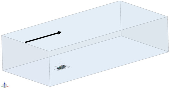
Figure 3.
Computational domain; arrow denotes flow direction going from left to right.
4.1. Mesh
The mesh was generated using the SnappyHexMesh utility in OpenFOAM, which takes Stereolithographic (.STL) files as inputs. Consequently, all vehicle parts and wind tunnel boundaries were exported as separate STL files, each later assigned its specific boundary conditions. The initial mesh generation involves creating a background mesh to fully encompass all vehicle parts and wind tunnel walls. Specifying the farthest corners of the rectangular domain, along with the number of cells in each direction, is critical for ensuring even sides of a single cell. This background mesh, termed level zero, represents the coarsest mesh in the entire domain, with a selected base mesh size of 0.25 m for this simulation.
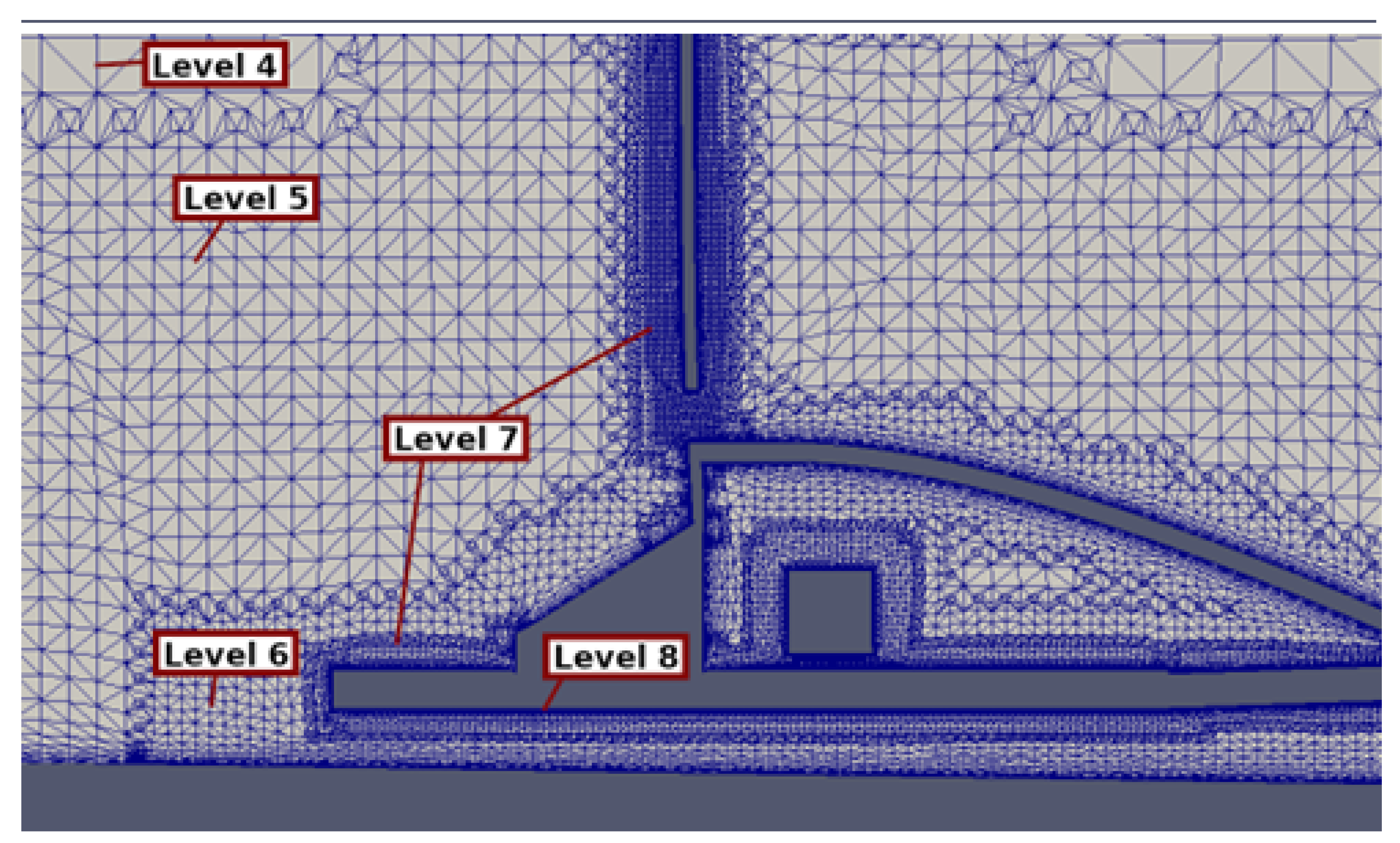
Mesh refinement occurs in levels, where each 3D cell is divided into eight cells. Level-one cells measure 0.125 m, level-two cells are 0.0625 m, and so forth. Refinement is achieved using volume sources, allowing resizing within specific geometries, and specifying the distance from an object, refining every cell within the specified distance to the assigned level. This combination of volume and distance refinement features was applied in all simulations. Figure 4 illustrates volume refinement regions. Surface refinement follows a similar fashion. Maximum and minimum cell levels are specified based on curvature parameters. The algorithm determines whether cell size should be closer to the minimum or maximum levels. High curvature results in surface refinement to the maximum specified level, while low curvature leads to refinement to the minimum level.
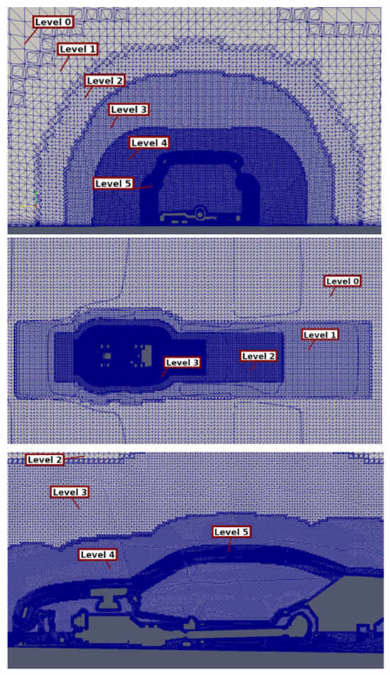
Figure 4.
Volume mesh and different mesh refinement levels; slices through (Top), (Middle), and (Bottom) planes.
Figure 5 (Top) provides a zoomed-in view of the volume mesh surrounding the car on the plane. This perspective illustrates the changing refinement levels as the distance from the car surface approaches zero. Notably, the volume beneath the car required refinement to levels 5 and 6 due to the presence of a high velocity gradient associated with the underbody center jet flow and its dissipation. Accurately capturing this jet dissipation is crucial for predicting force coefficients, as will be demonstrated in the Results section. Emphasizing the significance of refinement, the area around the front splitter takes precedence. This region experiences the highest pressure and velocity gradients. Consequently, the splitter-surface undergoes refinement to levels 7 and 8, resulting in a cell size of 1–2 mm. The volume is refined to level 7 (2 mm cell size); Figure 5 (Bottom) illustrates volume refinement around the splitter’s leading edge, ensuring a minimum of 10 cells vertically between the splitter and the ground.
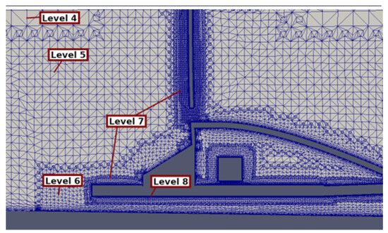
Figure 5.
Zoomed-in view of the volume mesh showing refinement levels at various distances forming the surface around the splitter region.
4.2. Boundary Conditions
Given that the average speed of the NASCAR Xfinity Series racecar on a 1.5-mile track is 180 mph, the simulation was conducted at this speed; this corresponded to an inlet uniform velocity of 80.5 m/s. To align with the real-world scenario, the ground velocity was set at the same magnitude and direction as the airflow. Tangential velocity on tire surfaces was assigned to match the ground speed, and all rotational components were configured with the same angular velocity as the tires. For the inlet conditions, a turbulence intensity (TI) of 0.2% and a turbulent viscosity ratio of 10 were selected to closely represent the aerodynamic environment of the wind tunnel test conditions. It is important to note that a TI of 0.2% is not representative of the environment an Xfinity racecar would experience on the track. However, since the CFD work involves validating the methodology against wind tunnel test data, the TI settings used are those typically expected in a wind tunnel.
For the inlet conditions, a turbulence intensity (TI) of 0.2% and a turbulent viscosity ratio of 10 were selected, ensuring a comprehensive representation of the aerodynamic environment of the wind tunnel test condition. Note that a TI of 0.2% is not a representative of the environment an Xfinity racecar would experience on a track; however, since the CFD work involves methodology validation against wind tunnel test conditions, TI conditions as would be expected in a wind tunnel are used.
4.3. Simulation Settings
Considering the huge mesh size and limited computing resources, conducting any simulation other than Reynolds-Averaged Navier–Stokes (RANS) is found impractical. Given the maximum local speed of the flow, which is below Mach 0.3, an incompressible SST RAN solver was used, as was previously used by Fu et al. [5], Jacuzzi [10], and Catranis [11]. However, previous studies indicated this turbulence model has a tendency to overpredict the wake region’s size and predict early separation. To address this, adjustments to turbulence closure coefficients were made which aligned the model predictions better with wind tunnel results.
The selection of a numerical discretization scheme is pivotal. Among the popular and robust schemes for external flow, first- and second-order upwind schemes were compared against wind tunnel experiments. Focusing on global force coefficients and surface flow patterns, both schemes closely predicted force coefficients, with the main distinction observed in surface flow patterns within separation regions. The second-order scheme closely resembled the wind tunnel experiment’s flow patterns, although it exhibited a larger separation bubble. In contrast, the first-order scheme failed to predict separation altogether. Consequently, the second-order scheme was chosen for subsequent simulations. Efforts will be made to rectify early separation through adjustments to the turbulence model and its coefficients.
The simulation involving radiator flow utilized Darcy’s law and porous media. Measurements of pressure drop and velocity ratios were conducted in front of and behind the radiator during the wind tunnel experiment. Utilizing this data, a pressure drop vs. bulk velocity relationship was developed, and the resultant coefficients were fed into the simulation parameters. This approach is similar to the one used by Zhang et al. [3], which showed very good correlation with experimental underhood flow. An interested reader is directed to the OpenFOAM User Guide [22] for additional reading and understanding on how this is implemented in OpenFOAM.
5. Results and Discussion
The performance comparison between the 2016 and 2017 versions of the racecar will be presented for two different configurations, specifically related to the ride height settings, a common term in motorsports terminology. These two ride heights are labeled as RH1 and RH2. RH1 represents a low-drag vehicle setting optimized for faster tracks, such as super-speedways with longer straightaways. In contrast, RH2 corresponds to a high-down-force setting suited for short and intermediate tracks. Typically, the low-drag setting (RH1) results in lower down-force compared to the high-drag, high-down-force setting (RH2). These different vehicle settings are achieved by adjusting both the heave and pitch of the racecar. However, the specific values for heave and pitch corresponding to these two ride heights are proprietary and confidential information belonging to the sponsor. Therefore, we are not permitted to disclose these data beyond the general description provided.
5.1. Tuning of SST Turbulence Model Closure Coefficients
The model closure coefficients used in popular Reynolds-Averaged Navier–Stokes (RANS) turbulence models are often selected in an ad hoc manner (see Pope [23]). To enhance the accuracy of RANS predictions for turbulent flows over simplified and realistic road vehicle geometries and racecars, several efforts have been made to tune these coefficients specifically for each geometry. For instance, Fu et al. [4,24] adjusted the model closure coefficients for the SST turbulence model applied to a Gen-6 NASCAR Cup racecar. Their approach involved systematically varying the coefficients through evenly spaced values, one at a time, to achieve improved predictions of lift- and drag-forces when compared to wind tunnel data. Similarly, Bounds et al. [25] refined the coefficients for a fully detailed automotive passenger vehicle. They varied the SST closure coefficients independently and then combined the optimal values to create the “best” set of coefficients. Overall, these tuning efforts aim to enhance the predictive accuracy of RANS turbulence models for various geometries by optimizing the model closure coefficients.
As previously mentioned, the SST turbulence model-based CFD simulations, using default closure coefficients, tend to overpredict the size of the wake region and predict early flow separation. The accurate prediction of these phenomena is crucial for the precise estimation of down-force coefficients, which is of paramount importance in racing applications. In the context of motorsports aerodynamics, the accurate prediction of down-force takes precedence over other parameters. Previous studies have indicated that the prediction of down-force heavily depends on the choice of turbulence model closure coefficients. However, a comprehensive study on the impact of all turbulence model closure coefficients is beyond the scope of this research. Therefore, we focused on studying the impact of the parameter (see Equation (10)), which is related to the determination of eddy viscosity, on the prediction of backlight separation and overall aerodynamic headline predictions. Note that we emphasized the accuracy of down-force prediction more than the prediction of drag. Also, note that all forces are presented as a nondimensional force coefficient defined as:
In Equation (16), A, , and stand for the reference area, fluid density, and freestream velocity, respectively; is the force such as drag-force (D), down-force or negative lift (L), and side-force S. We further note the following:
- The quantities and represent the lift-force components as experienced at the center of the front- and rear-wheel axles, respectively, and are known as the Front Lift-Force Coefficient and Rear Lift-Force Coefficient, respectively.
- The quantity % Front is defined as the ratio of the Front Lift-Force to the Total Lift-Force.
- The quantity represents the ratio of the negative lift-force (down-force) to drag-force.
For the purpose of demonstrating the efficacy of our SST turbulence model closure coefficients tuning endeavor, the headline aerodynamic coefficients for this car at ride height H1 are obtained by running CFD simulations with the coefficient set to both the default value of 0.31 and a wide range of modified values in which we observed that produces the best result. These results, with set at 0.31 and 0.50, are compared against wind tunnel (WT) measurements in Table 1. In this table, Delta CFD and WT data represent the differences between CFD predictions and wind tunnel measurements, expressed as a percentage of the wind tunnel data. A positive value of “Delta CFD and WT” indicates an overprediction by CFD, while a negative value indicates an underprediction by CFD. Clearly, from Table 1, with set to 0.50, CFD predictions show much better correlation with the experimental data across all quantities. Except for an approximately 10% difference in the drag prediction, the lift- and side-force coefficients show errors of around 1%. From our motorsports experience, this level of correlation between CFD and experimental data is considered outstanding. Even for the drag, —0.50 results in a 4% reduction in underprediction. Changing from 0.31 to 0.50 improved the overall lift prediction by as much as 10%; while the front lift prediction shows a 7% improvement, the rear shows almost an 11% improvement. However, note that while the default value of produced an underprediction of both front and rear down-force, setting equal to 0.50 showed a 1.7% overprediction.

Table 1.
CFD predicted headline aerodynamic coefficients obtained using default SST closure coefficients compared against wind tunnel data.
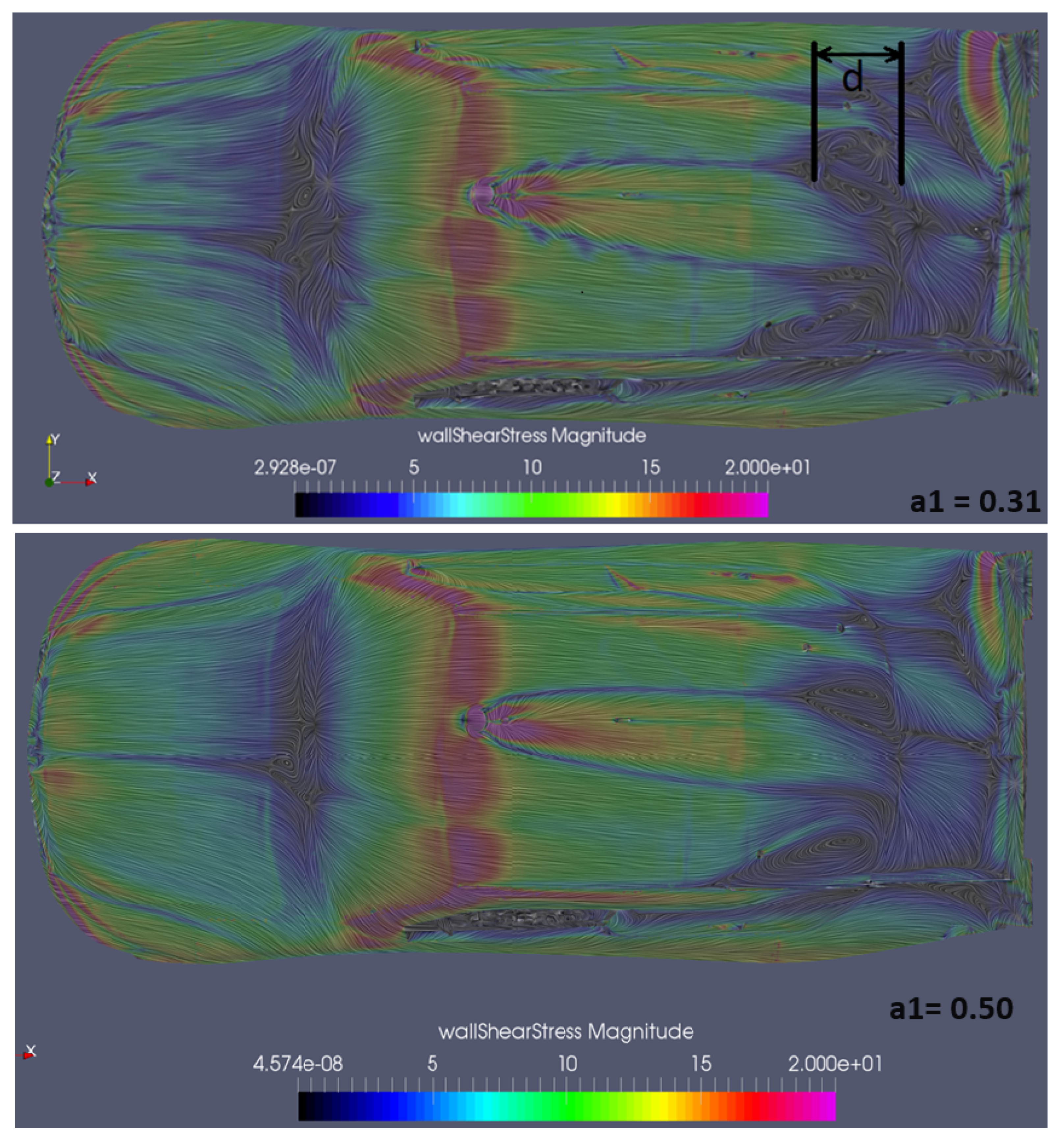
To understand why a larger value of produces such accurate results, we need to revisit our earlier comment: the key lies in correctly predicting the backlight separation bubble. To illustrate this, Figure 6 shows oil-flow lines and surface wall stress contours obtained with set to 0.31 and 0.50. Note that, strictly speaking, these “oil-flow lines” are actually “surface streamlines”. However, they are commonly referred to as oil-flow lines in the NASCAR community to better correspond with their experimental counterparts. In Figure 6 (Top), the size of the separation bubble, marked as d, is compared against the separation bubble observed during wind tunnel tests. When was set to 0.31, the CFD-predicted backlight separation bubble was found to be approximately 30% larger than what was observed in the tests. To decrease the separation, turbulent viscosity needs to increase in the wake region. According to Equation (10), the simplest way to achieve this is by increasing the value of . When was set to 0.50, our CFD simulations predicted a backlight separation bubble that closely matched the experimental observations, as can be seen in Figure 6 (Bottom).
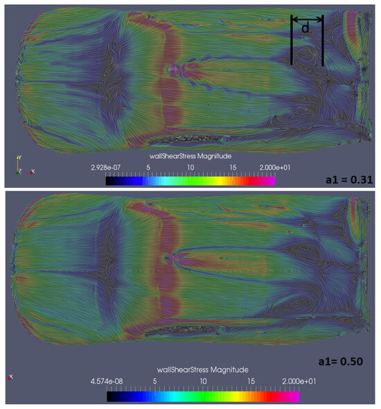
Figure 6.
Oil-flow lines superimposed on wall shear stress contour, as obtained from CFD simulations using default (Top) and modified (Bottom) values of .
5.2. Mesh Independence
The literature abundantly demonstrates that mesh size can significantly influence CFD simulation results, with this influence diminishing asymptotically as the mesh size increases beyond a certain optimum threshold, which is highly case-dependent. There is a tendency for diminishing returns as the cost–benefit ratio of running higher resolution simulations outweighs the benefits of further mesh refinement beyond a certain point. Thus, to ensure the mesh used was sufficiently or optimally refined, numerous simulations were performed using different level-zero cell sizes while keeping other mesh parameters constant; note that for this study simulations were run using the 2016 car at ride height RH1. Specifically, simulations were conducted with level-zero cell sizes of 0.29 m, 0.27 m, and 0.25 m, resulting in overall mesh sizes of 77 million (M) cells, 95 M cells, and 123 M cells, respectively. These results are presented in Table 2, in which it can be observed that refining the mesh beyond 94 M cells did not yield significant improvements in the results. For instance, changing the mesh size from 77 M to 123 M cells had minimal impact on the drag- and side-force coefficients, with variations not exceeding 4 counts. However, the lift coefficient was more sensitive to mesh size changes. Increasing the mesh size from 77 M to 95 M cells, which is approximately a 20% increase, resulted in a 1.6% change in the lift coefficient. Further increasing the cell count by another 20%, to 123 M cells, showed only a 0.35% difference in the lift coefficient prediction.

Table 2.
Mesh independence check for the 2016 car at R1 ride height.
Considering the computational resources required, a 123 M cell mesh demands 20% more CPU hours compared to a 95 M cell mesh. However, the results obtained using the fine mesh (123 M cells) and the medium mesh (95 M cells) were within 0.35% of each other. Therefore, the 94 M cell mesh was deemed optimal, providing a good balance between accuracy and computational efficiency. This detailed analysis ensures that the selected mesh size is sufficiently large to produce reliable results without unnecessarily increasing computational costs. The 95 M cell mesh offers an optimal solution, achieving high accuracy in lift coefficient prediction while maintaining manageable computational resource requirements.
5.3. Comparison of 2016 and 2017 Racecar Aerodynamics Characteristics at Ride Height RH2
A CFD simulation framework that produces aerodynamic headline coefficient predictions with strong correlation to experimental results and independence from mesh size has been successfully established. This robust simulation setup allowed for the validation of the modified turbulence model under varying conditions; the stage is now set to use this setup to gain insight into the difference between the aerodynamic characteristics of the 2016 and 2017 racecars. However, to further validate the simulation configuration, the vehicle’s ride height was set to RH2, and the results were compared to wind tunnel experiments. Changing the ride height of the car significantly affects the flow characteristics around the vehicle. Variations in ride height can alter the distribution of aerodynamic forces, impacting lift-, drag-, and side-forces. Therefore, it is crucial to maintain good correlation between the CFD simulation and experimental results to ensure the reliability and accuracy of the modified turbulence model under different conditions.
The ride height RH2 represents a different aerodynamic setup compared to the initial configuration (RH1), introducing new challenges for the simulation. Ensuring that the modified turbulence model can accurately predict the aerodynamic behavior at RH2 is essential for validating the overall simulation approach. This step demonstrates the model’s capability to handle changes in vehicle configuration and provides confidence in its predictive power for various aerodynamic scenarios.
Table 3 compares the CFD predicted force coefficients data against wind tunnel data for both the 2016 and 2017 versions of the racecar corresponding to ride height R2. These coefficients include lift-, drag-, and side-forces, which are critical for assessing the vehicle’s aerodynamic performance. This table shows a high level of agreement between the CFD and experimental results at RH2 and validates the modified turbulence model’s accuracy and reliability. This validation is crucial for ensuring that the simulation can be used for further aerodynamic analyses and optimization of the vehicle’s performance. Similar to previous results, the drag coefficient is underpredicted by about 7.6% and 10.7% for the 2016 and 2017 cars, respectively. On the positive side, down-force and side-force have great correlation with experimental results along with the prediction of front-to-rear down-force balance. Interestingly, as shown in Table 3, the total down-force (or negative lift) for the 2016 car is overpredicted by CFD by about 2.4%. In contrast, the 2017 car simulations show a 3.4% underprediction of down-force. For the 2016 car, the front down-force is almost perfectly predicted by CFD, while the rear down-force is overpredicted by 5%. Conversely, for the 2017 car, CFD underpredicts both front and rear down-force, with the rear down-force predictions showing a better correlation (1.2% error) compared to the front down-force prediction (6%). Notably, for both cars, CFD underpredicts the front balance by 1.2%. Regarding side-force prediction errors, the 2017 car simulation shows an almost perfect correlation with wind tunnel data, while the side-force for the 2016 car is underpredicted by about 7%.

Table 3.
CFD prediction and wind tunnel test data for headline aerodynamic coefficients for both 2016 and 2017 racecars at ride height R2.
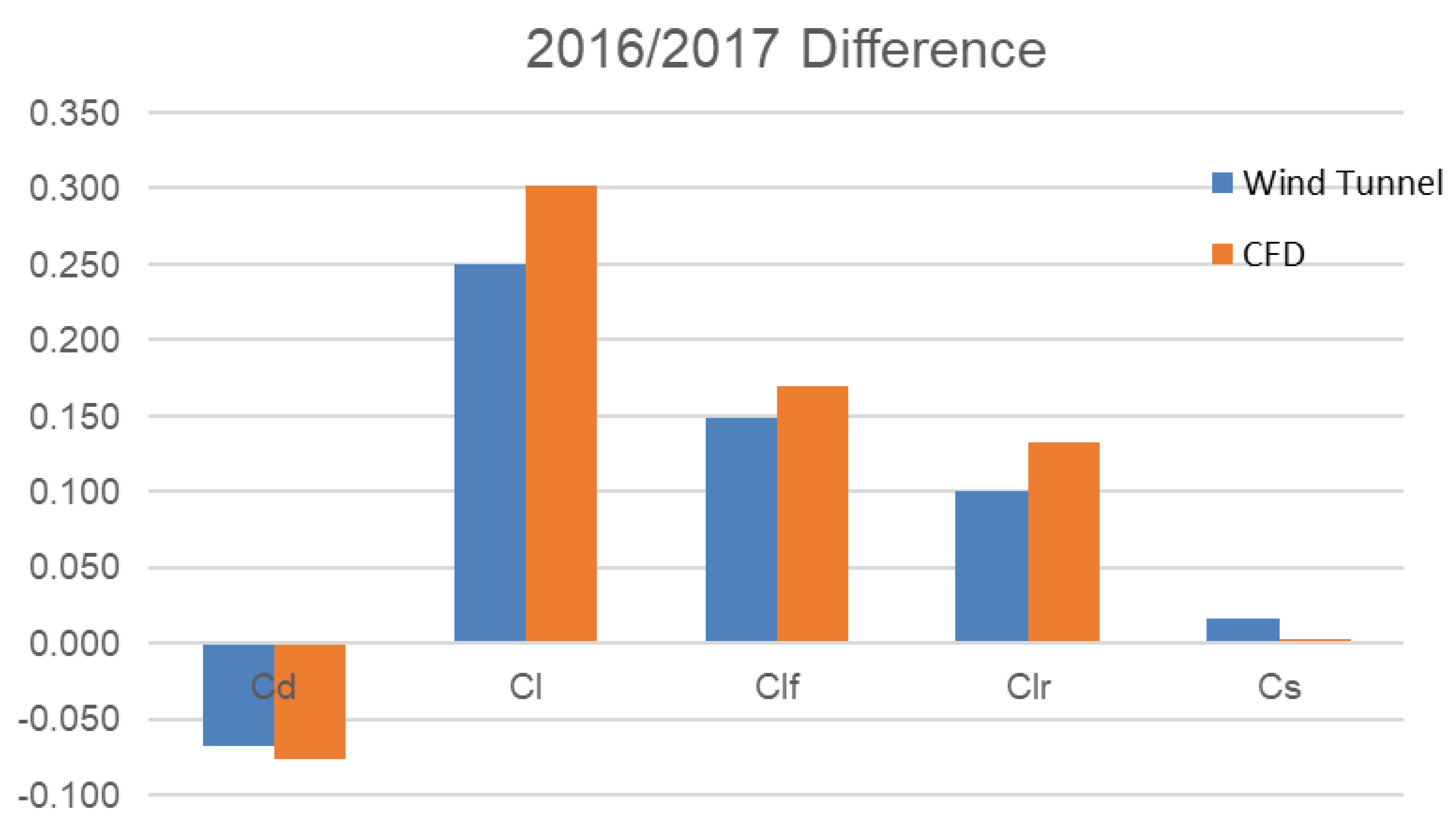
To provide a clearer visualization of the differences in the aerodynamic characteristics between these two cars, the numerical data presented in Table 3 are summarized in Figure 7. This summary is based on our Computational Fluid Dynamics (CFD) simulations and wind tunnel tests. The figure offers a more intuitive comparison, making it easier to understand the variations in aerodynamic performance between the two models. As observed in this figure, both the CFD simulations and wind tunnel tests indicate that the 2017 car exhibits lower drag. The CFD results show a slightly higher drag difference of 76 counts compared to 68 counts observed in the wind tunnel tests. However, this discrepancy is not significant from an engineering decision making perspective, as both CFD and wind tunnel data exhibit the same directional trend. Likewise for the lift predictions; although trend-wise both CFD and WT tests show higher lifts or lower down-force for the 2017 car as compared to the 2016 car, CFD results tend to somewhat amply the delta; this trend is true for total, front, and rear lift components. For example, while CFD indicates a total down-force decrease of 302 counts for the 2017 car, the wind tunnel shows a decrease of 250 counts.

Figure 7.
Aerodynamic characteristic differences between 2016 and 2017 cars from CFD simulations and wind tunnel tests.
However, the greatest discrepancy between the CFD prediction and WT test in terms of the performance delta between 2016 and 2017 cars is seen in the side-force. While the wind tunnel shows a 17-count decrease in side-force, CFD shows only a 2-count decrease. Note that, for the 2017 car, the difference between the CFD predicted and experimentally observed side-force is only one count or about 0.5%; the difference for the 2016 car is significantly larger, about 14 counts or almost 7%. As such, the underproduction of delta side-force between the 2016 and 2017 cars may arise from the CFD prediction error for the 2016 car. Although we cannot be very certain here, one of the possible reasons could be the inability of the steady-state RANS CFD approach to capture the bi-stable nature of wakes commonly observed in a a ground vehicle (see [26,27,28] for details). This bi-stability is a transient phenomenon which can greatly influence the side-force component and cannot be characterized in a steady-state simulation. Additionally, the possibility of vehicle misalignment during the wind tunnel test cannot be ruled out. Even a small change in the yaw angle of the vehicle could easily result in a 14-count difference in side-force, which highlights the sensitivity of the aerodynamic measurements to precise vehicle positioning and alignment in the test setup. However, without further proof, which is left for a future investigation, this hypothesis and the possibility of other sources of measurement errors can merely be treated as a conjecture only.
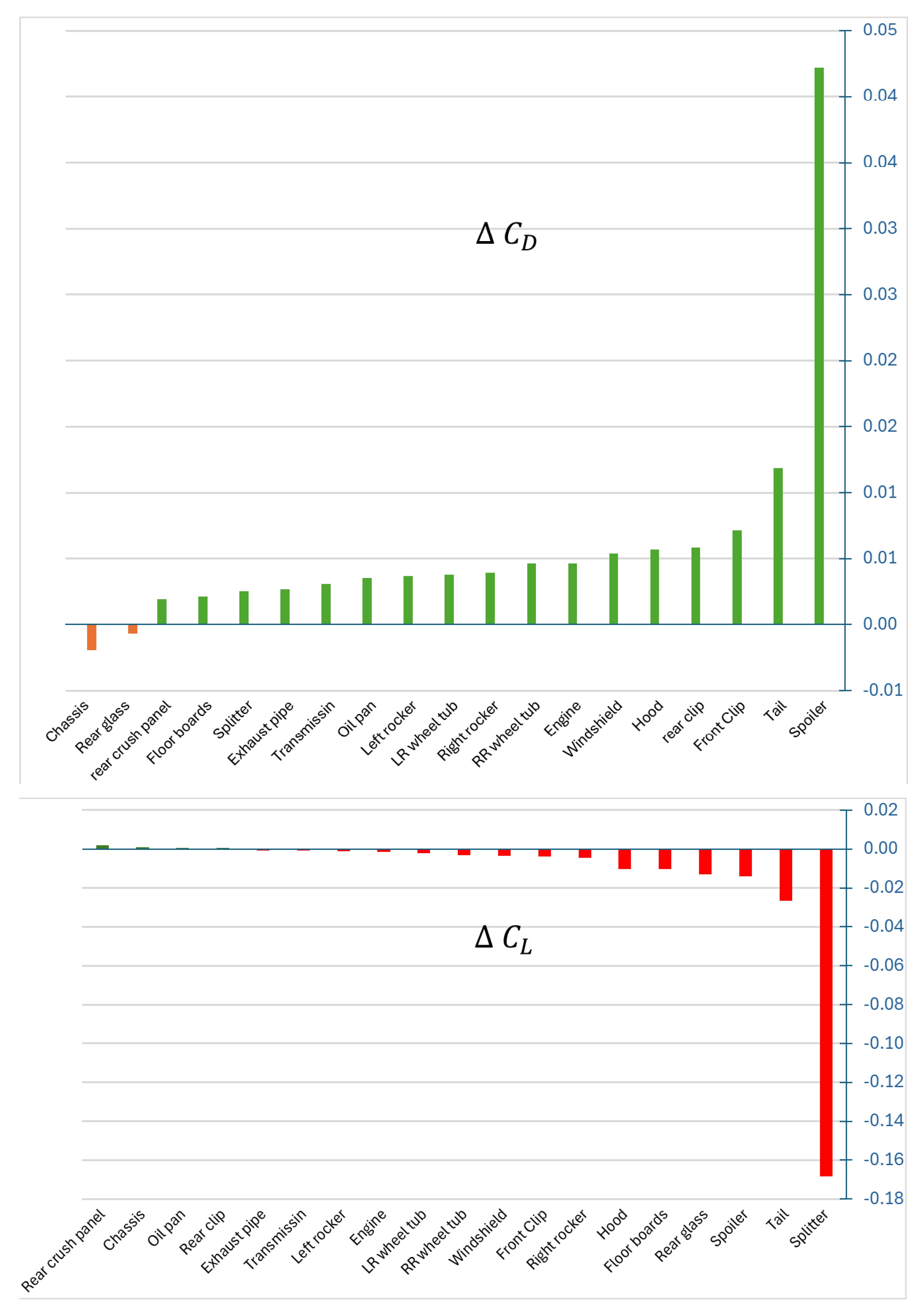
Next, we will investigate the contributions from different components of the racecar towards the changes in drag coefficient () and lift coefficient () between the two racecar packages. Here, is defined as the difference between the 2016 car’s and the 2017 car’s , where X can be either the drag (D) or lift (L) force. These values are illustrated in Figure 8. It is important to note that this analysis cannot be conducted in a wind tunnel, highlighting the utility of CFD simulations. In Figure 8, “Green” indicates decreases and “Red” indicates increases in the coefficient values due to the introduction of the 2017 car. Thus, a positive component value signifies lower drag due to that component in the 2017 package, while a negative component value indicates an increase in lift (or decrease in down-force) due to that component.
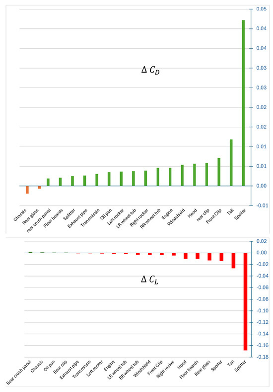
Figure 8.
The contributions of the different components of the racecar to (Top) and (Bottom) between the 2016 and 2017 configurations.
From Figure 8 (Top), it is clear that the majority of the drag reduction is attributed to changes in the spoiler. Out of the total 68 counts of drag difference between the two cars, 42 counts are due to the spoiler, followed by the tail with 12 counts and the front clip with 7 counts. Other contributors to the drag reduction include the rear clip and hood (6 counts each), windshield, engine bay, and right rear wheel tub (5 counts each), right rocker, left rear wheel tub, and left rocker (4 counts each), and oil pan, transmission, exhaust pipe, and splitter (3 counts each). Notably, the chassis and rear glass add 2 counts and 1 count of drag increase, respectively. Although almost two-thirds of the drag reduction is due to the changes in the spoiler configuration for the 2017 car, this modification only contributes 26 counts out of the 302 counts of down-force reduction, which is about 9%. The majority of the drag reduction, 168 counts or about 55%, comes from changes in the splitter configuration, which only causes 3 counts or about 4% of drag reduction. Other notable contributors to the increase in lift are the tail (26 counts), the rear glass (13 counts), and the floorboard and hood (10 counts each). Interestingly, for the 2017 package, the rear crash panel reduces lift by 2 counts. Additionally, the chassis, oil pan, and rear clip each contribute to a lift reduction of 1 count.
Next, we will further analyze the differences in the aerodynamic behaviors of these two packages by examining surface pressure distribution, static pressure probe measurements, and the underbody jet. The underbody jet is considered one of the most critical factors contributing to down-force generation for this racecar.
5.3.1. Surface Pressure Distribution
The static pressure distribution in terms of on the upper surface of both cars is shown in Figure 9. Note that with P and representing local static pressure and reference pressure, respectively, the static pressure coefficient, , is defined as:
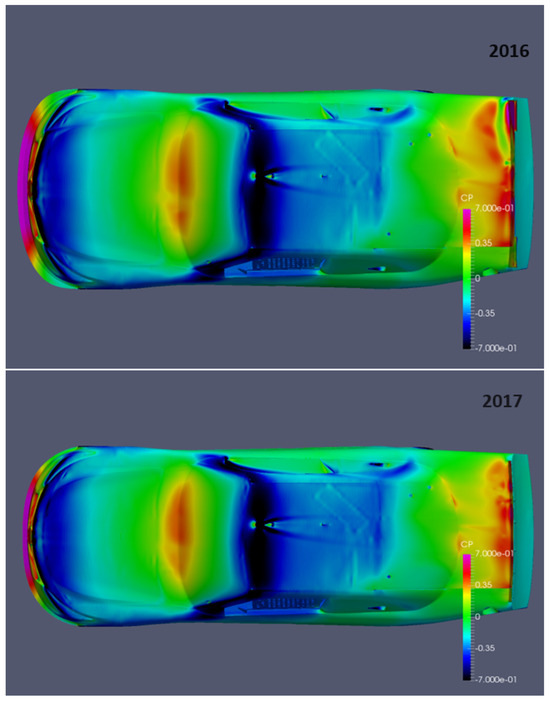
Figure 9.
Static pressure coefficient () distribution on the upper surface of the 2016 (Top) and 2017 (Bottom) cars.
Overall, no significant differences are observed between the two cars, except in the decklid area near and around the spoiler base region. In this region, a strong asymmetry in pressure distribution is evident for the 2016 car, with the right side showing much lower static pressure near the spoiler base. Additionally, the static pressure on the decklid of the 2016 car is considerably higher, resulting in a higher for the 2016 car.
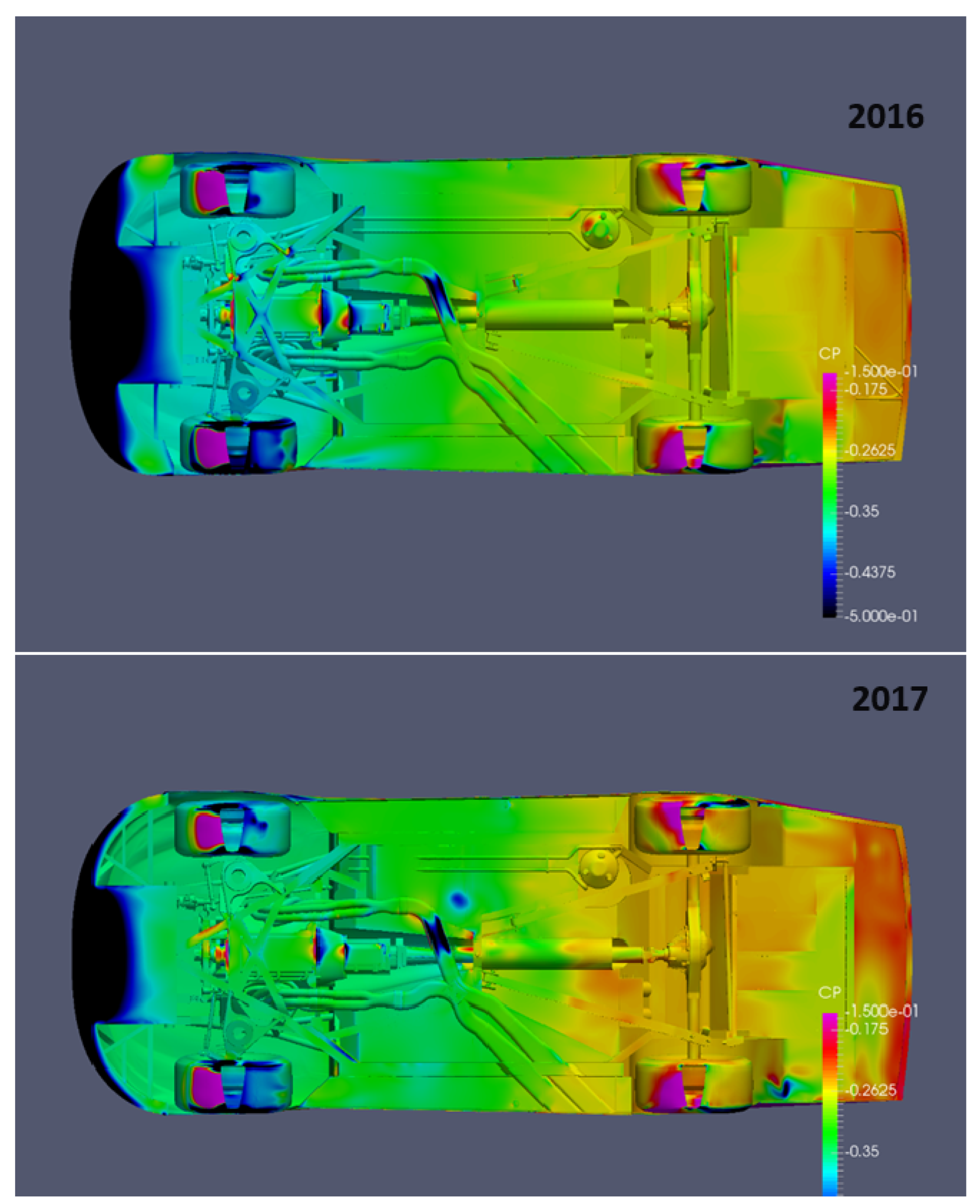
Although the observed differences in the static pressure distribution over the decklid partially explain why the 2016 car has higher rear down-force, they do not fully account for the large difference in front down-force between the two cars. The less discernible pressure distribution differences on the front part of the upper surface fail to explain this disparity. Therefore, it is important to examine the underbody pressure distribution for both cars, as shown in Figure 10. The figure reveals distinct differences in pressure distribution between the two racecars. Notably, the 2016 car exhibits a much larger area of suction (negative ) in the splitter and surrounding region, attributable to the longer extent of the splitter plate. This increased underbody suction significantly contributes to the higher front down-force of the 2016 car. Additionally, rearward of the floorboard midsection, a stronger suction is observed for the 2016 car. This, combined with the higher positive pressure on the decklid, results in a greater rear down-force for the 2016 car.
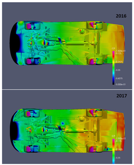
Figure 10.
Static pressure coefficient () distribution on the underbody surface of the 2016 (Top) and 2017 (Bottom) cars.
5.3.2. Pressure Probe Measurements
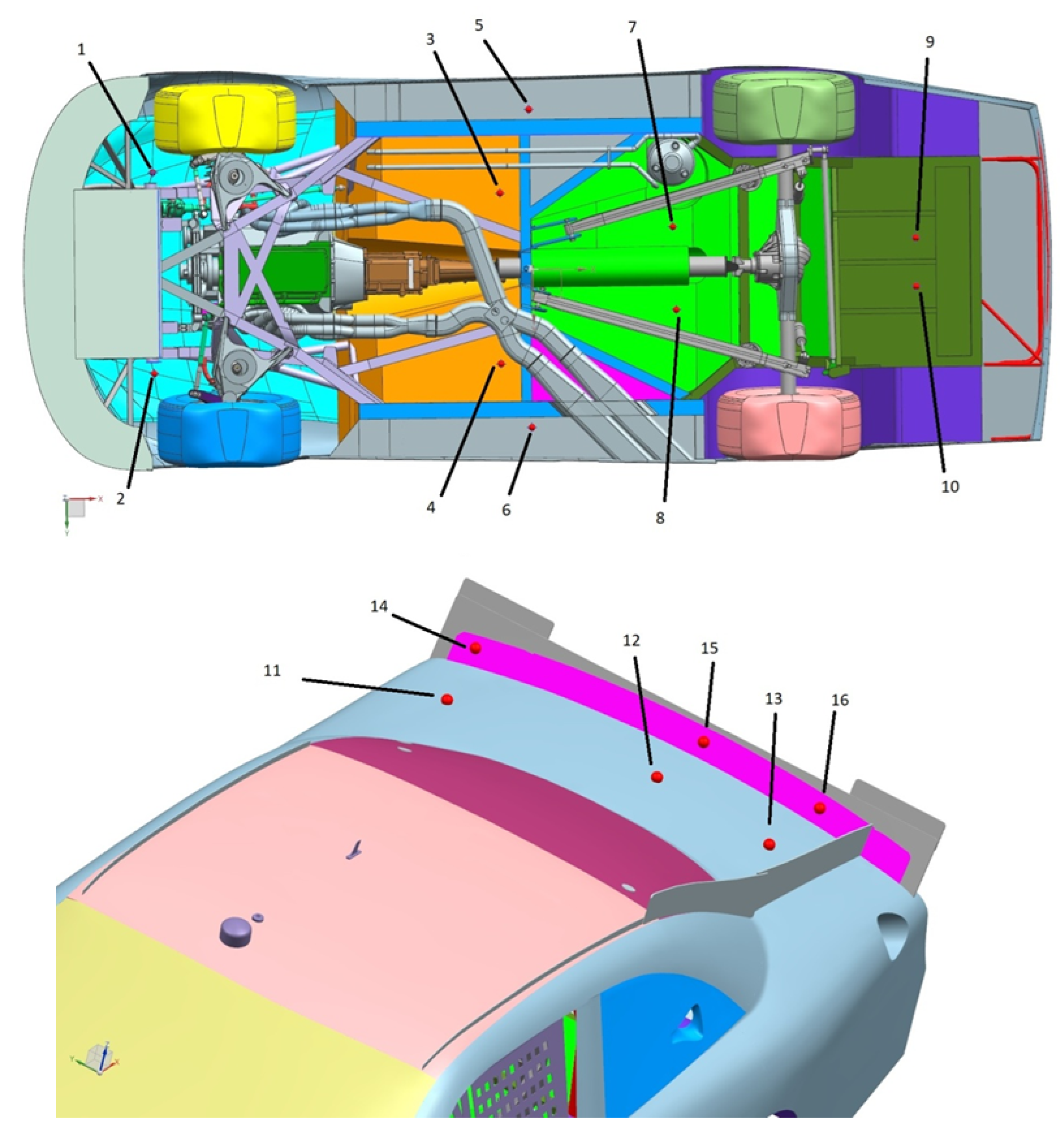
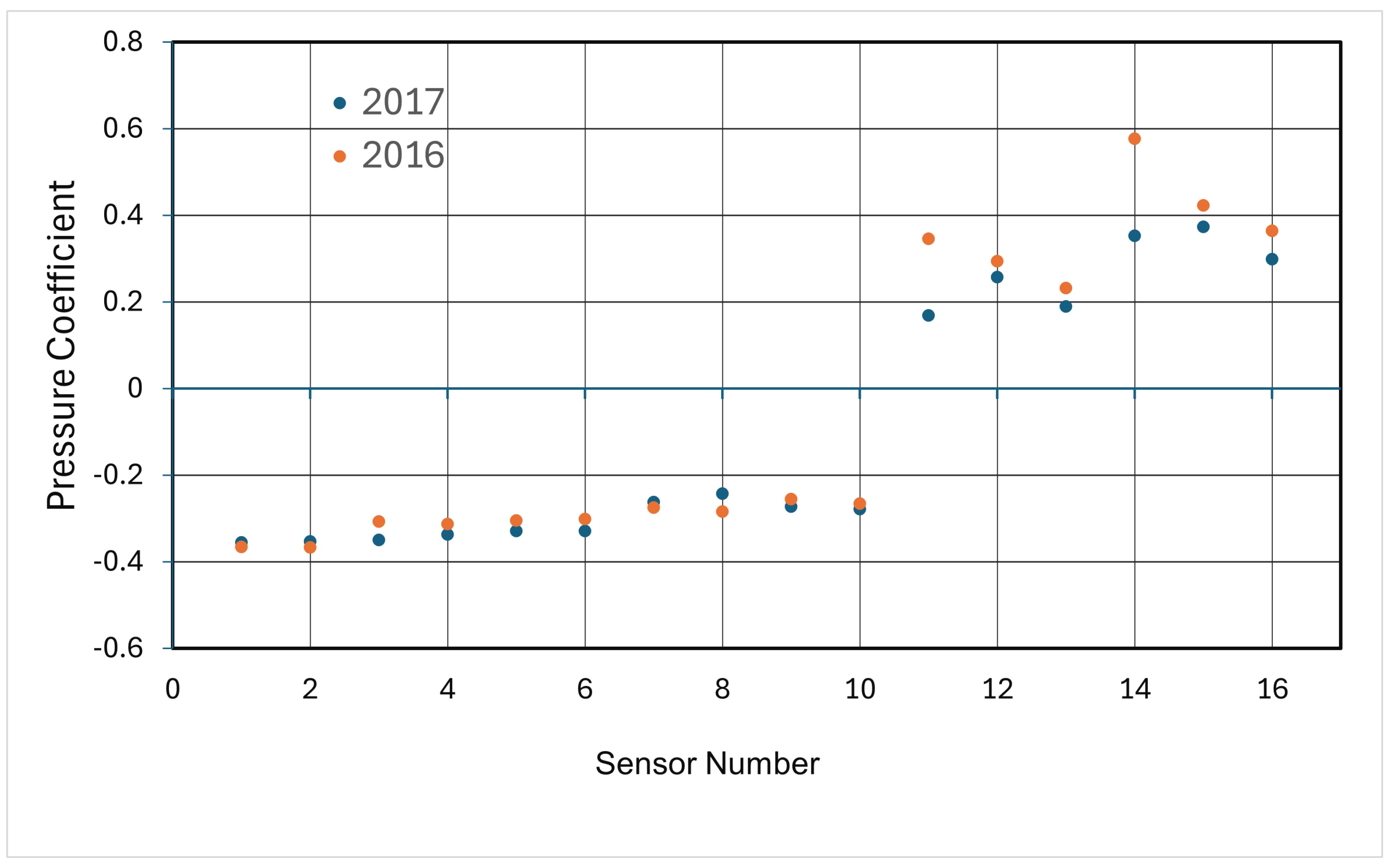
To further quantify the differences in distribution between the two cars, a total of sixteen pressure probes were placed: ten on the underbody (probe numbers 1–10) and six on the decklid (probe numbers 11–16), as shown in Figure 11. The results of static probe pressure data are shown in Figure 12.

Figure 11.
Locations of the pressure probes. Please note that in the bottom figure, the 2017 spoiler is overlaid on the 2016 spoiler in pink to better illustrate the locations of the pressure probes.
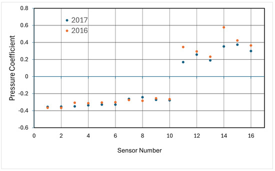
Figure 12.
Pressure probe data.
Based on the data from sensors 1 and 2, in Figure 12, the 2016 rule package results in lower pressure under the hood. Given the large surface area of the hood, even a small decrease in pressure translates into a significant increase in down-force, quantified as an increase of 10 counts in favor of the 2016 car. Similarly, the 2016 car exhibited higher pressure under the rocker panels and the front floorboards. This pressure decreased under the rear floorboards before increasing again under the fuel cell. Although the floorboards as a whole did not show significant pressure changes between the 2016 and 2017 cars, the extensive surface area of the floorboards means that even minor pressure decreases can have a notable impact on down-force. Consequently, the average small pressure decrease contributed to an additional 10 counts of down-force on the 2016 car. Pressure data from probes 11–16 indicate that the 2016 car exhibits significantly higher positive pressure on the decklid at all selected locations. Although probes 9 and 10 reveal slightly lower underbody suction for the 2016 car compared to the 2017 car, the substantially greater positive pressure on the upper surface of the decklid results in higher rear down-force for the 2016 car. This combination of pressure distributions clearly explains the increased rear down-force observed in the 2016 car, despite the minor reduction in underbody suction. The higher positive pressure on the decklid plays a crucial role in enhancing the overall aerodynamic performance, resulting in improved down-force characteristics. These findings highlight the importance of understanding pressure distributions across various regions of the car’s body, as even minor variations can significantly impact overall aerodynamic performance.
5.3.3. Underbody Jet Velocity
As mentioned earlier, the dynamics of the underbody center jet flow are considered a critical aspect of the flow field by the stock car racing aerodynamics community. This flow significantly impacts the generation of down-force, which is essential for the racecar’s performance and stability. Down-force improves tire grip and handling, allowing the car to maintain higher speeds through corners and enhancing overall control. In light of this, understanding the underbody center jet characteristics is crucial. Figure 13 compares the underbody center jet flow dynamics of the two cars. Clearly, the longer side-wise extent of the 2016 car helps to keep the center jet energized and coherent for a longer distance. In contrast, for the 2017 configuration, the center jet dissipates much earlier. Specifically, the center jet in the 2017 car dissipates completely at a distance of about 1.3 m downstream of the car’s center, leading to an increase in pressure as measured at probe locations 7 and 8. This comparison reveals how different design elements and aerodynamic packages influence the flow patterns beneath the car, directly affecting the pressure distribution and, consequently, the down-force. By analyzing these characteristics, engineers can identify areas for improvement and optimize the aerodynamic setup to achieve better performance. The insights gained from such analyses underscore the importance of detailed pressure distribution studies across various regions of the car’s body. Even minor variations can significantly influence the overall aerodynamic performance, demonstrating the need for precise and comprehensive aerodynamic evaluations in the development and refinement of high-performance racecars.
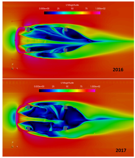
Figure 13.
Velocity distribution under the car at , where h is the splitter-gap, for the 2016 (Top) and 2017 (Bottom) cars.
5.4. The Bottom Line: Race Track Performance Comparison
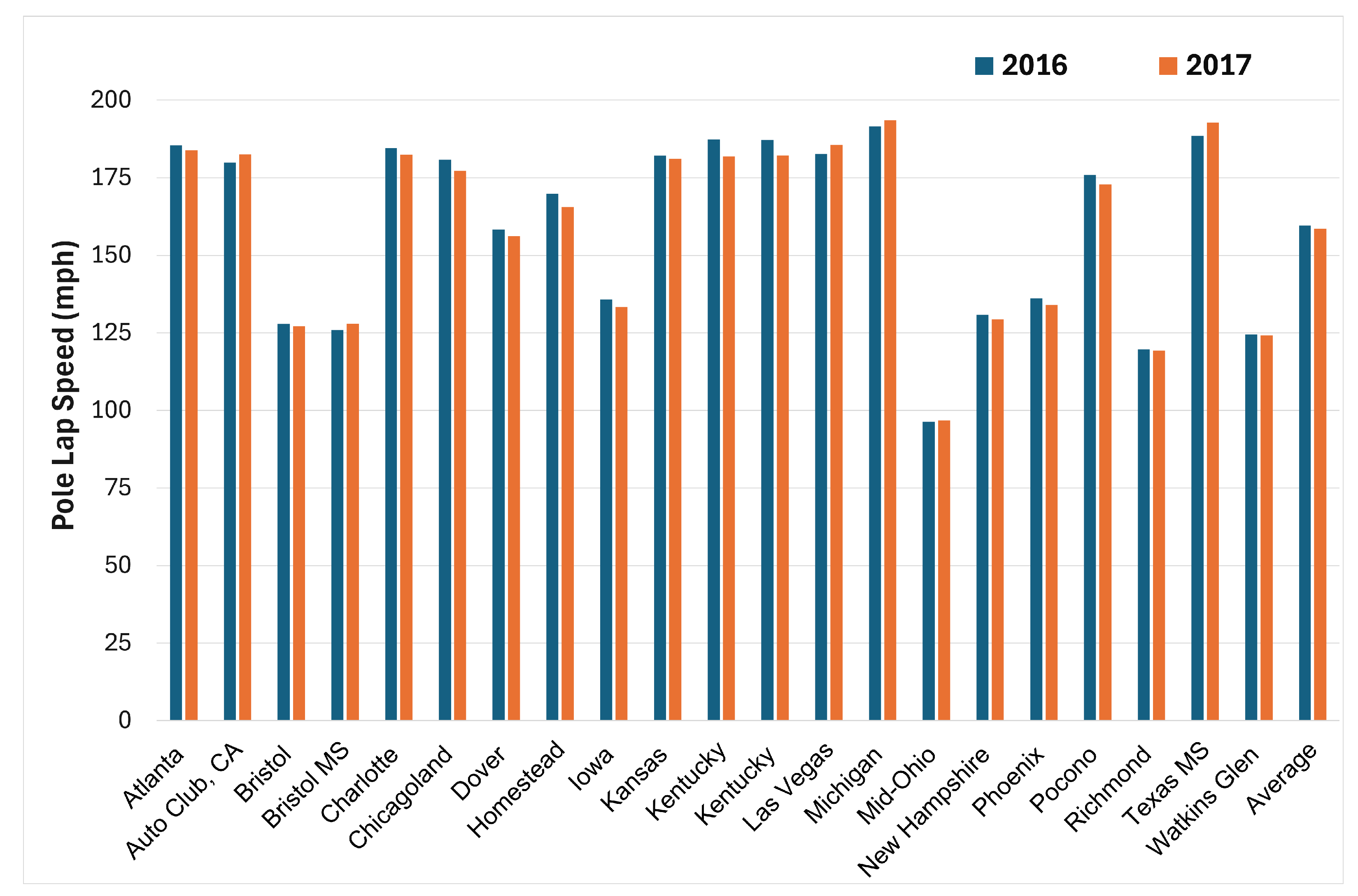
How do these changes translate to actual racing performance? Clearly, the lower drag of the 2017 car means it will be faster on the straights. However, the reduced down-force means this car will be much slower in the corners. To understand the overall effect, a comparison of pole lap speeds for the two cars at selected race tracks is presented in Figure 14; the presented data come from actual 2016 and 2017 race records. In racing terminology, “pole lap speed” refers to the average lap speed of a driver who sets the fastest lap time in qualifying for a race. Some tracks, such as Daytona International Speedway (Florida), Talladega Superspeedway (Alabama), and Indianapolis Motor Speedway (Indiana), were not included in the comparison due to different aerodynamic rules applying to these tracks. The track at Fort Worth, Texas, was resurfaced before the beginning of the 2017 season and thus was excluded from the comparison. Bristol, Tennessee, was also excluded because a traction compound was added to the race track surface in the 2017 season. Other races were not accounted for because either in the 2016 or 2017 season, qualifying was canceled.
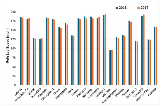
Figure 14.
Pole speed for different race tracks as recorded during 2016 and 2017 race seasons. Source: Jayski’s NASCAR Silly Season Site; https://www.jayski.com/xfinity-series/2016-nascar-xfinityseries-race-results/ for 2016 car and https://www.jayski.com/xfinity-series/2017-nascar-xfinityseries-race-results/ for 2017 car (accessed on 31 August 2024).
We all know that weather can affect lap speeds, making it challenging to compare lap speeds for different packages individually from track to track. Therefore, it is more reasonable to compare average pole lap speeds. After the introduction of the 2017 aerodynamic rules, cars, on average, went 1.225 mph slower per lap. This proves the importance of down-force for race vehicle performance. The reduction in down-force for the 2017 car, while beneficial for straight-line speed due to lower drag, ultimately resulted in slower lap times due to decreased cornering speed. This highlights the critical role that down-force plays in the overall performance and competitiveness of race cars.
We need to add a word of warning regarding the complexity of the relationship between CFD results and track performance. The connection between the CFD results and the average lap speeds achieved is not adequately substantiated in our paper, as it uses just two ride heights, and our comments regarding lower drag and higher top speeds, as well as lower down-force and reduced cornering speeds, present an overly simplistic view of a track-based vehicle’s performance. Furthermore, a more comprehensive understanding and higher confidence predictions require additional results for various ride heights since a racecar’s ride height changes dynamically as it traverses the track, affecting its aerodynamic performance. Thus, utilizing only one or two ride heights does not fully represent the conditions experienced by a racecar on the track. However, we believe that the above discussion still offers value by providing at least a partial picture of the differences in and causes of aerodynamic performance. While this section does not present a complete analysis, it serves as an initial step in highlighting the relationship between aerodynamic properties and vehicle performance on the track. Thus, this section can be seen as a foundation for future, more comprehensive studies that could include a broader range of ride heights and additional variables such as cross-wind.
6. Conclusions
OpenFOAM, as an open-source software, allowed for extensive customization to meet specific simulation needs for turbulent flow around a NASCAR Xfinity Racing Series stock car, particularly for comparing the aerodynamic characteristics of the 2016 and 2017 racecars. Complex meshes were created, and simulations were performed, with a mesh sensitivity study ensuring the accuracy of the results. Adjustments to turbulence model coefficients improved correlation with wind tunnel data. Simulations at two ride heights—RH1 (lower drag for faster tracks) and RH2 (higher down-force)—demonstrated strong agreement with wind tunnel results, validating the accuracy of comparing different aerodynamic packages.
The 2017 aerodynamic rules led to a significant reduction in down-force and drag, primarily due to a shorter rear spoiler and a smaller front splitter, which altered the underbody flow and increased pressure under the car. Simulations aligned well with wind tunnel measurements for down-force and side-force but showed discrepancies in drag prediction, indicating a need for further study. Improved correlation could be achieved by using pressure probes during wind tunnel tests to refine turbulence models and boundary conditions.
The lower drag coefficient allowed for faster acceleration on straights but required greater deceleration due to reduced down-force, stressing the braking system. Despite these changes, racing quality did not noticeably improve, leading to a return to a high-down-force and high-drag package in the 2019 NASCAR Monster Energy Cup Series to enhance competitiveness. As of the 2019 season, NASCAR Xfinity Racing Series rules remained unchanged. This experience underscores the importance of balancing aerodynamic efficiency with overall race performance through continuous adaptation and optimization.
Author Contributions
Conceptualization, N.O. and M.U.; methodology, N.O. and M.U.; software, N.O.; validation, N.O. and M.U.; formal analysis, N.O. and M.U.; investigation, N.O. and M.U.; resources, N.O. and M.U.; data curation, N.O.; writing—original draft preparation, M.U.; writing—review and editing, M.U.; visualization, N.O.; supervision, M.U.; project administration, M.U.; funding acquisition, M.U. All authors have read and agreed to the published version of the manuscript.
Funding
This project was supported through a finding from Joe Gibbs Racing, Huntersville, NC, 28078, U.S.A.
Data Availability Statement
The wind tunnel test data presented in this paper, along with the specific racecar geometry employed in the simulations, constitute confidential property owned by Joe Gibbs Racing. Acquisition of these proprietary assets was facilitated through a binding Non-disclosure Agreement (NDA). Consequently, the authors are constrained from publicly disseminating the complete set of test and geometry data, as well as the resulting Computational Fluid Dynamics (CFD) simulation data, beyond the results, images, and discussions presented in this paper.
Acknowledgments
The authors thankfully acknowledge funding support from Joe Gibbs Racing, Huntersville, NC, 28078, U.S.A., through which Nazarii Olkhovskyi was supported as a Graduate Research Assistant to work on this project. Additionally, the authors express their appreciation to Joe Gibbs Racing for supplying the vehicle geometry and wind tunnel test data, without which this project would not have been possible.
Conflicts of Interest
The authors declare no conflicts of interest.
Abbreviations
The following abbreviations are used in this manuscript:
| CFD | Computational Fluid Dynamics |
| DDES | Delayed Detached Eddy Simulation |
| DES | Detached Eddy Simulation |
| DMD | Dynamic Mode Decomposition |
| DNS | Direct Numerical Simulation |
| GV | ground vehicle |
| GVSC | Ground Vehicles Systems Center |
| IDDES | Improved Delayed Detached Eddy Simulation |
| LES | Large Eddy Simulation |
| POD | Proper Orthogonal Decomposition |
| PSD | Power Spectral Density |
| RANS | Reynolds-Averaged Navier–Stokes |
| Reynolds Number | |
| RMS | Root Mean Squared |
| ROM | Reduced Order Method |
| SGS | Sub Grid Scale |
| SRS | Scale Resolved Simulation |
| SST | Shear Stress Transport |
| SVD | Singular Value Decomposition |
| TD | Time Dynamics |
| VWT | virtual wind tunnel |
| WT | wind tunnel |
References
- The Editors of Encyclopedia Britannica. Stock-Car Racing. Encyclopedia Britannica. 2023. Available online: https://www.britannica.com/sports/stock-car-racing (accessed on 12 October 2023).
- Swansey, J.D., Jr. NASCAR America: The Myth and Melodrama of White Masculinity in Stock Car Racing’s National Vision. Bachelor’s Thesis, Wesleyan University, Middletown, CT, USA, 2021. [Google Scholar]
- Zhang, C.; Uddin, M.; Song, X.; Fu, C.; Foster, L. Simultaneous Improvement of Vehicle Under-Hood Airflow and Cooling Drag Using 3D CFD Simulation; Technical Report, SAE Technical Paper; SAE: Warrendale, PA, USA, 2016. [Google Scholar]
- Fu, C.; Bounds, C.; Uddin, M.; Selent, C. Fine Tuning the SST k − ω Turbulence Model Closure Coefficients for Improved NASCAR Cup Racecar Aerodynamic Predictions. SAE Int. J. Adv. Curr. Pract. Mobil. 2019, 1, 1226–1232. [Google Scholar] [CrossRef]
- Fu, C.; Bounds, C.P.; Selent, C.; Uddin, M. Turbulence modeling effects on the aerodynamic characterizations of a NASCAR Generation 6 racecar subject to yaw and pitch changes. Proc. Inst. Mech. Eng. Part D J. Automob. Eng. 2019, 233, 3600–3620. [Google Scholar] [CrossRef]
- Misar, A.; Davis, P.; Uddin, M. On the Effectiveness of Scale-Averaged RANS and Scale-Resolved IDDES Turbulence Simulation Approaches in Predicting the Pressure Field over a NASCAR Racecar. Fluids 2023, 8, 157. [Google Scholar] [CrossRef]
- Misar, A.S.; Uddin, M. Effects of Solver Parameters and Boundary Conditions on RANS CFD Flow Predictions over a Gen-6 NASCAR Racecar; Technical Report, SAE WCX Technical Paper; SAE: Warrendale, PA, USA, 2022. [Google Scholar]
- Misar, A.S.; Uddin, M.; Pandaleon, T.; Wilson, J. Scale-Resolved and Time-Averaged Simulations of the Flow over a NASCAR Cup Series Racecar; Technical Report, SAE Technical Paper; SAE: Warrendale, PA, USA, 2023. [Google Scholar]
- Jacuzzi, E.; Barrier, A.; Granlund, K.O. NASCAR race vehicle wake modification via passive blown ducts and its effect on trailing vehicle drag. In Proceedings of the 2018 AIAA Aerospace Sciences Meeting, Kissimmee, FL, USA, 8–12 January 2018; p. 0558. [Google Scholar]
- Jacuzzi, E.; Granlund, K. Passive flow control for drag reduction in vehicle platoons. J. Wind Eng. Ind. Aerodyn. 2019, 189, 104–117. [Google Scholar] [CrossRef]
- Catranis, D. Correlation of Cloud Based Computational Fluid Dynamics Simulations to Wind Tunnel Test Results for a NASCAR XFINITY Series Vehicle. Master’s Thesis, Indiana University Purdue University Indianapolis, Indianapolis, IN, USA, 2018. [Google Scholar]
- Olkhovskyi, N. CFD Based Analysis of the EffectsS of 2017 NASCAR Xfinity Racing Series Aerodynamic Rule Changes. Master’s Thesis, The University of North Carolina at Charlotte, Charlotte, NC, USA, 2019. [Google Scholar]
- Menter, F.R. Two-equation eddy-viscosity turbulence models for engineering applications. AIAA J. 1994, 32, 1598–1605. [Google Scholar] [CrossRef]
- Menter, F. Zonal two equation kω turbulence models for aerodynamic flows. In Proceedings of the 23rd Fluid Dynamics, Plasmadynamics, and Lasers Conference, Orlando, FL, USA, 6–9 July 1993; p. 2906. [Google Scholar]
- Zhang, C.; Bounds, C.P.; Foster, L.; Uddin, M. Turbulence modeling effects on the CFD predictions of flow over a detailed full-scale sedan vehicle. Fluids 2019, 4, 148. [Google Scholar] [CrossRef]
- Menter, F.R.; Kuntz, M.; Langtry, R. Ten years of industrial experience with the SST turbulence model. Turbul. Heat Mass Transf. 2003, 4, 625–632. [Google Scholar]
- Wilcox, D.C. Reassessment of the scale-determining equation for advanced turbulence models. AIAA J. 1988, 26, 1299–1310. [Google Scholar] [CrossRef]
- Wilcox, D.C. Turbulence modeling for CFD; DCW Industries: La Canada, CA, USA, 2006; Volume 34. [Google Scholar]
- Jones, W.P.; Launder, B.E. The prediction of laminarization with a two-equation model of turbulence. Int. J. Heat Mass Transf. 1972, 15, 301–314. [Google Scholar] [CrossRef]
- Launder, B.E.; Sharma, B.I. Application of the energy-dissipation model of turbulence to the calculation of flow near a spinning disc. Lett. Heat Mass Transf. 1974, 1, 131–137. [Google Scholar] [CrossRef]
- Fu, C.; Uddin, M.; Zhang, C. Computational Analyses of the Effects of Wind Tunnel Ground Simulation and Blockage Ratio on the Aerodynamic Prediction of Flow over a Passenger Vehicle. Vehicles 2020, 2, 318–341. [Google Scholar] [CrossRef]
- CFD Direct. OpenFOAM v6 User Guide. 2018. Available online: https://doc.cfd.direct/openfoam/user-guide-v6/ (accessed on 6 June 2024).
- Pope, S.B. A perspective on turbulence modeling. In Modeling Complex Turbulent Flows; Springer: Berlin/Heidelberg, Germany, 1999; pp. 53–67. [Google Scholar]
- Fu, C.; Uddin, M.; Robinson, C.; Guzman, A.; Bailey, D. Turbulence models and model closure coefficients sensitivity of NASCAR Racecar RANS CFD aerodynamic predictions. SAE Int. J. Passeng. Cars-Mech. Syst. 2017, 10, 330–345. [Google Scholar] [CrossRef]
- Bounds, C.P.; Zhang, C.; Uddin, M. Improved CFD prediction of flows past simplified and real-life automotive bodies using modified turbulence model closure coefficients. Proc. Inst. Mech. Eng. Part D J. Automob. Eng. 2020, 234, 2522–2545. [Google Scholar] [CrossRef]
- Aultman, M.; Duan, L. Flow Topology of the Bi-Stable Wake States for the DrivAer Fastback Model. Flow Turbul. Combust. 2024, 113, 217–247. [Google Scholar] [CrossRef]
- He, K.; Minelli, G.; Wang, J.; Dong, T.; Gao, G.; Krajnović, S. Numerical investigation of the wake bi-stability behind a notchback Ahmed body. J. Fluid Mech. 2021, 926, A36. [Google Scholar] [CrossRef]
- Bai, H.; Xia, C.; Yu, L.; Fan, Y.; Jia, Q.; Yang, Z. Effects of Rear Slant Angles on the Bi-Stable Behavior of the Ahmed Body; Technical Report, SAE Technical Paper; SAE: Warrendale, PA, USA, 2024. [Google Scholar]
Disclaimer/Publisher’s Note: The statements, opinions and data contained in all publications are solely those of the individual author(s) and contributor(s) and not of MDPI and/or the editor(s). MDPI and/or the editor(s) disclaim responsibility for any injury to people or property resulting from any ideas, methods, instructions or products referred to in the content. |
© 2024 by the authors. Licensee MDPI, Basel, Switzerland. This article is an open access article distributed under the terms and conditions of the Creative Commons Attribution (CC BY) license (https://creativecommons.org/licenses/by/4.0/).


