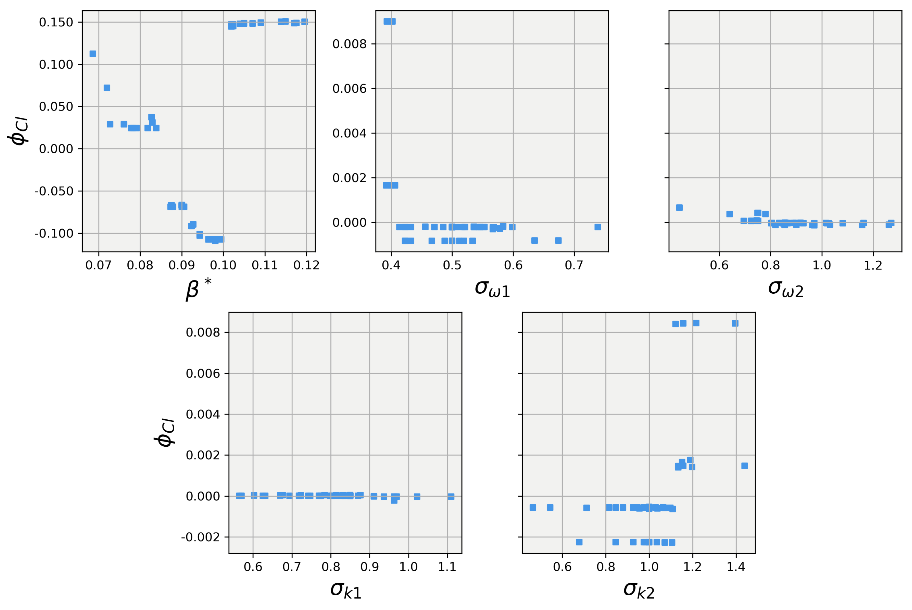
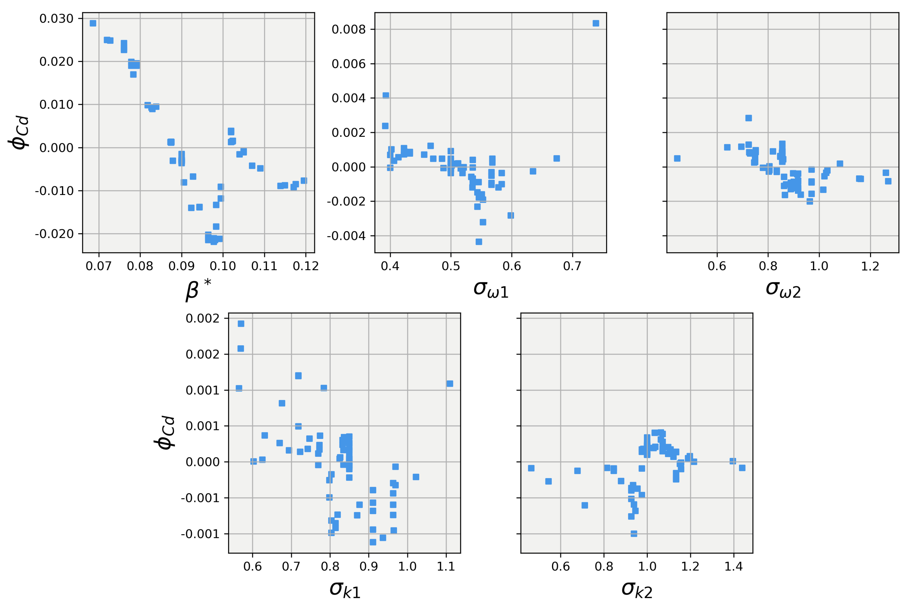
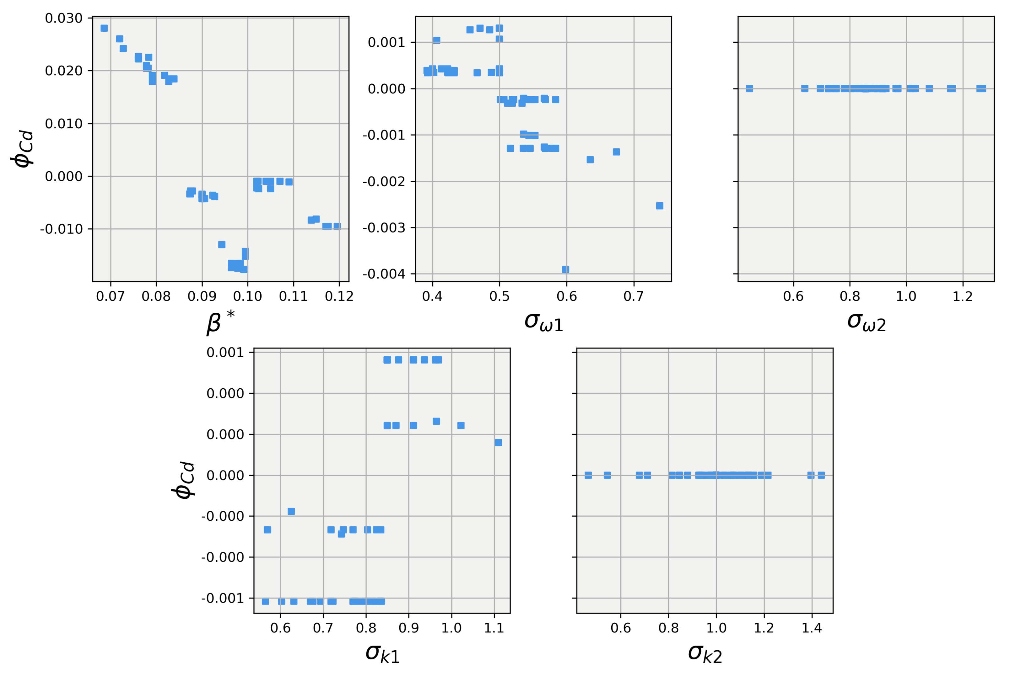
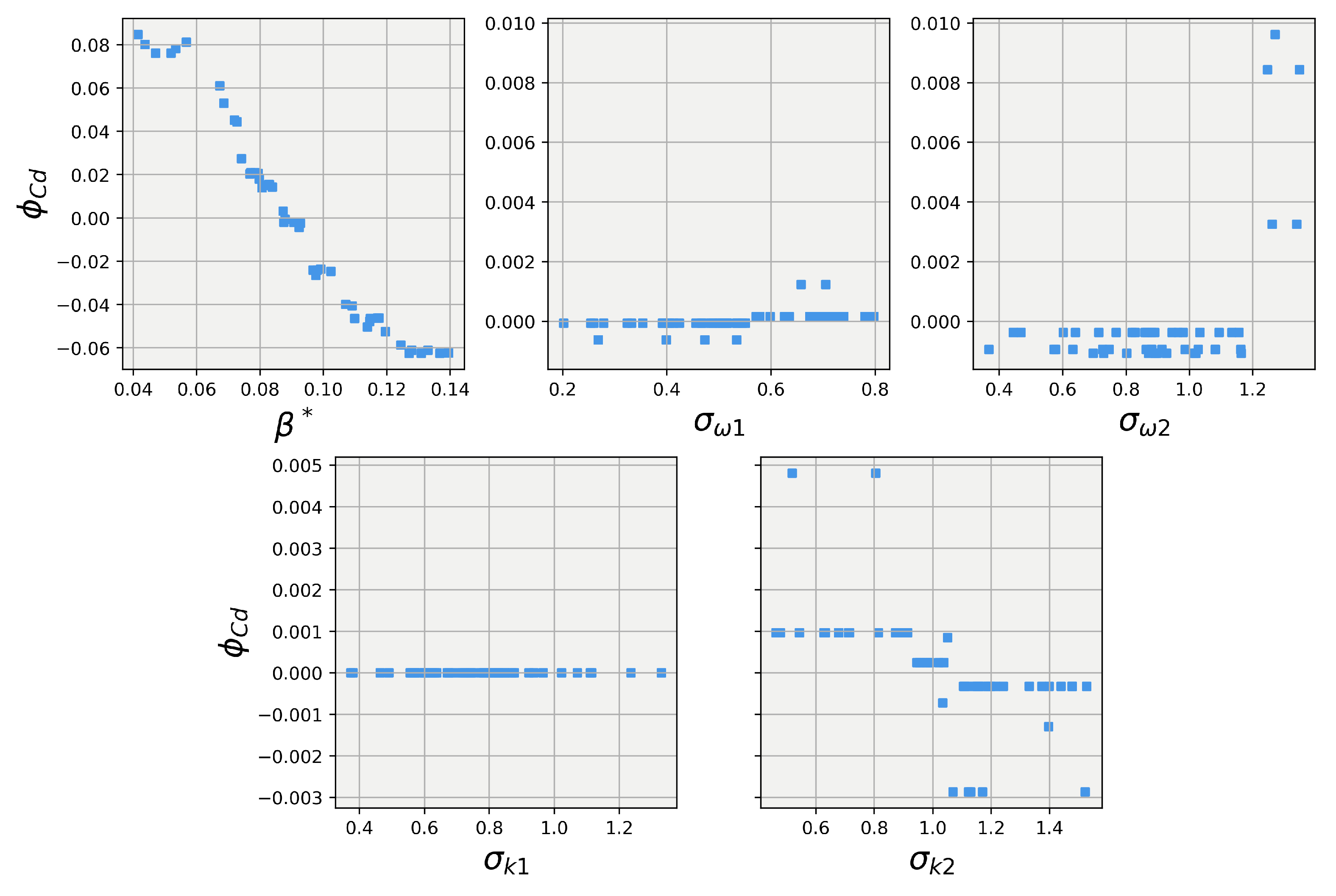
Abstract
Computational fluid dynamic (CFD) models and workflows are often developed in an ad hoc manner, leading to a limited understanding of interaction effects and model behavior under various conditions. Machine learning (ML) and explainability tools can help CFD process development by providing a means to investigate the interactions in CFD models and pipelines. ML tools in CFD can facilitate the efficient development of new processes, the optimization of current models, and enhance the understanding of existing CFD methods. In this study, the turbulent closure coefficient tuning of the SST Reynolds-averaged Navier–Stokes (RANS) turbulence model was selected as a case study. The objective was to demonstrate the efficacy of ML and explainability tools in enhancing CFD applications, particularly focusing on external aerodynamic workflows. Two variants of the Ahmed body model, with 25-degree and 40-degree slant angles, were chosen due to their availability and relevance as standard geometries for aerodynamic process validation. Shapley values, a concept derived from game theory, were used to elucidate the impact of varying the values of the closure coefficients on CFD predictions, chosen for their robustness in providing clear and interpretable insights into model behavior. Various ML algorithms, along with the SHAP method, were employed to efficiently explain the relationships between the closure coefficients and the flow profiles sampled around the models. The results indicated that model coefficient had the greatest overall effect on the lift and drag predictions. The ML explainer model and the generated explanations were used to create optimized closure coefficients, achieving an optimal set that reduced the error in lift and drag predictions to less than 7% and 0.5% for the 25-degree and 40-degree models, respectively.
1. Introduction
In computational fluid dynamics (CFD), accurately and efficiently modeling turbulent flow fields presents a formidable challenge. In the ever-continuing goal of improving the prediction veracity of CFD models, machine learning (ML) presents a promising solution by creating adaptable statistical models. ML involves developing statistical models that can tailor their predictions to the data presented during training. The models ‘learn’ incrementally as more data are added to the training set, much in the same way that a human learns [1]. This incremental learning capability enables the ML model to adjust its predictions to better fit the training dataset and improve its accuracy without human intervention.
ML models can be broadly classified into two categories based on the type of training data they use: supervised learners and unsupervised learners. Supervised learners use labeled training data, meaning that each training instance has an associated ‘correct’ answer. The ML dataset comprises features (the inputs to the model) and targets (the desired outputs of the model). During training, the model makes predictions that are compared to the known outputs (targets). The error between the predicted and actual values is then used to adjust the model until the desired accuracy is achieved. In contrast, unsupervised learning does not use labeled targets. Instead, the model identifies patterns and groups the data into clusters based on trends observed in the training features. During training, the unsupervised model optimizes a loss function, typically a distance metric, to group the data effectively. Again, applications of ML models in supervised learning fall into two categories: regression, where a continuous output is predicted, and classification, where a discrete output is predicted. Unsupervised models are typically applied to clustering problems, where the objective is to group the data into clusters and learn from these groupings.
Linear regression is perhaps the simplest form of an ML model. It uses supervised learning to create a regression method, where each feature is combined in a linear sum, as shown in Equation (1). In this model, each input is multiplied by a weight and then summed with the other features to produce the final output. While this model is very simple, it does hold an additional advantage: it is interpretable. In the context of ML, an interpretable model is one where the inner structure and weights of the model can be used to explain in human terms the relationship of the features to the output of the model [2].
Interpretability in models is highly desired because it enables researchers to troubleshoot more effectively by detecting biases and gaining insights into the real-world system being modeled. This enhanced understanding results in greater trust among end-users, ultimately leading to increased adoption. For an ML model to be acceptable, its predictions need to be explained. Humans naturally seek order and develop notions of how things should occur, making the ability to explain predictions crucial for understanding and trust [3]. If a model contradicts the user’s preconceived notions, they will expect an explanation for this discrepancy to reconcile with their understanding. The challenge is that as model complexity increases, its ability to capture more complex trends and solve harder problems improves, but its interpretability decreases. At the extreme, the model becomes a black box, meaning only the inputs and outputs are visible to the user. In many real-world applications, model complexity has surpassed the point of being interpretable to meet the demands of the application. This lack of interpretability is often highlighted as a significant concern by many researchers. For example, Guidotti et al. [4] discussed how, in the 1970s, ML black-box models were discriminating against ethnic communities, even when no ethnic information was provided as a feature. The model used surnames as a proxy for ethnicity, highlighting how models can discover unintended trends in the data. For critical applications, a model should not be fully trusted until it can be explained. Guidotti et al. further stated that the explanation of a model can serve two primary purposes: to validate the model by revealing biases and to uncover the reasoning behind predictions so that actions based on those predictions can be better understood. Thus, the need for interpretability in complex models has led to the study of explainability. In the ML context, explainability is the process of explaining, in human terms, the relationship between a model’s features and outputs without revealing its inner weights and structure.
The present work focuses on model-agnostic approaches of explainability, since they can be applied to any model, including CFD models. Although CFD models are not black boxes, they are often not easy to interpret due to their complexity, particularly due to the non-linear interactions of the parameters involved in the transport and modeled equations. While their inner structure can be analyzed, explaining them in terms and simplicity so that humans can understand can be very challenging. Some may argue that CFD models are interpretable, but Doshi-Velez et al. [2] and Ribeiro et al. [5,6] emphasize that for true explainability, humans must be able to understand it easily. This means that if a model has too many parameters or a formulation that is too complex, like CFD governing equations, even an inherently interpretable model, such as a linear model, can become uninterpretable.
One of the first model-agnostic methods of explainability to gain great popularity is popularly known as the local interpretable model-agnostic explanations, or LIME for short, which was introduced by Ribeiro et al. [5,6] as a solution for explaining a model’s prediction based on a given feature set X. LIME takes random samples of the model around the prediction to be explained by perturbing the feature set. The samples are then weighted based on their distance from the prediction of interest, with closer samples being given more weight. These weighted samples are then used to find a sparse linear model, known as the explainer model, that fits the perturbations by optimizing a loss function. Once the model has been fit to the data, the inherent interpretable nature of linear models is leveraged to explain the more complex model. This is done by using the weights of the linear model, which can directly relate the inputs to the output. To keep the number of features low when selecting a linear model, a penalty function is introduced, which penalizes explainer models that use many features. By penalizing models that use many features, LIME can present concise explanations that can be easily explained to a human. LIME has been successfully applied in various fields such as picture classification, text topic recognition, and ensemble-based decision trees.
Another earlier approach to creating model-agnostic explanations comes from Štrumbelj et al. [7,8,9], who proposed that Shapley values, a concept from game theory [10], could be utilized to generate model-agnostic explanations. Shapley values are a method of determining a player’s (a feature) marginal contribution to the outcome (the model’s output) of a game (the model) when participating in a coalition (a set of features). Although not a ML algorithm, Shapley values can serve as a tool to explain the predictions of a model. However, this Shapley value approach proved to be a very costly way to calculate the explanations. This led Štrumbelj et al. to develop an efficient sampling technique to approximate the Shapley values [8]. They proposed that the Shapley values approximation can be generated by sampling the training dataset without the need to retrain the model, which is a very important step for models that have long training times. This approach significantly reduces the sampling required for traditional Shapley values; however, a large dataset is still necessary to explain the model’s predictions.
Lundberg et al. [11,12] introduced a model-agnostic approach to explainability known as Shapley additive explanations (SHAP) that utilized the concepts of additive feature attribution (AFA) methods. In this work, Lundberg et al. demonstrated that many of the popular model explanation methods, such as LIME, deepLIFT [13], and Shapely values, are all based on the same framework of AFA. They were then able to build on this framework of AFAs and show that Shapley values are the key solution to the principle postulates of AFAs. Therefore, methods that do not follow the Shapley values principles are not true AFA methods, and sacrifice accuracy in their explanations. From this, they proposed SHAP, a modified version of LIME that aligns with the principles of Shapley value game theory. This adaptation led to a marked improvement in sampling efficiency compared to prior methods, along with greater congruence with human intuition than the standard LIME methodology. This caused SHAP to quickly become one of the most popular explainability methods in the ML space.
To better understand the context of this paper and the subsequent discussions, it is essential to review the current advancements and challenges in the field of external aerodynamics for ground vehicles, particularly regarding the accuracy and applicability of CFD approaches and best practices. In the past three decades, CFD has gained significant traction as a complementary tool to traditional wind tunnel testing for optimizing ground vehicle aerodynamic design. This trend is driven by CFD’s lower operational costs and faster turnaround times, which facilitate the rapid iteration and development of aerodynamic concepts without the need for expensive physical prototypes. Furthermore, CFD provides a comprehensive analysis of flow fields, offering insights into local flow phenomena that are not easily captured by wind tunnel tests, which typically focus on macroscopic aerodynamic properties such as force and moment coefficients. Despite these advantages, several challenges remain in the application of CFD to ground vehicle aerodynamics. These include the accurate modeling of complex turbulent flows, the need for high-fidelity simulations to capture intricate flow details, and the validation of CFD results against experimental data to ensure reliability. Addressing these challenges is critical for enhancing the predictive capability of CFD and ensuring its effective integration into the aerodynamic design process.
Recent advancements in computing power, particularly in terms of cost and affordability, combined with increasing demand from various industries, have led to a significant surge in the implementation of artificial intelligence (AI) and machine learning (ML) technologies in general. Following a similar trend, the field of computational fluid dynamics (CFD) is also beginning to incorporate ML, proving valuable in improving predictions and assisting with post-processing tasks. Despite its potential, the full extent of ML’s capabilities in CFD has yet to be fully explored and exploited. Most applications of ML in CFD have focused on developing new, high-fidelity turbulence models [14,15,16,17,18] or enhancing CFD discretization schemes [19,20] or solvers [21,22]. While these areas show great promise, they also have significant challenges. New models require vast amounts of high-fidelity data, which are often impractical to obtain, and improvements in solvers remain largely untested in real CFD applications. In contrast, the potential of using ML and AI to aid in traditional CFD processes and turbulence model development has shown promise but remains largely untapped. This paper aims to demonstrate the utility of one such ML/AI tool through a practical example of CFD turbulence model closure coefficient tuning. Specifically, the authors intend to highlight the power of explainability and ML as tools for CFD development by focusing on the problem of the Reynolds-averaged Navier–Stokes (RANS) turbulence model closure coefficient tuning.
The Reynolds-averaged Navier–Stokes (RANS) approach stands as one of the most extensively employed methodologies in CFD, enjoying wide prevalence across an array of engineering applications. However, it is acknowledged that RANS, while offering computational efficiency and speed, is relatively less precise for automotive flow simulations in comparison to alternative strategies like variants of detached eddy simulation (DES), a point underscored by Ashton [23,24]. Moreover, the efficacy of RANS can be compromised by issues pertaining to accuracy and repeatability, stemming from artifacts associated with the parallelization paradigm inherent in finite volume-based computational methods (refer to the work by Misar et al. [25]). Despite these acknowledged limitations, the computational efficiency intrinsic to RANS allows for simulations to be run within reasonable timeframes, aligning well with the swift design cycles necessitated by the automotive industry, particularly in the realm of motorsports encompassing entities like FIA Formula 1 and NASCAR. However, it is noteworthy that while RANS enjoys popularity, advancements in RANS modeling have been relatively stagnant in recent years in spite of the proactive endeavors spearheaded by the National Aeronautics and Space Administration (NASA) aimed at fostering and propelling technological evolution; see Slotnick et al. [26]. Prominently, recent efforts to improve RANS modeling have hinged on augmenting the precision and reliability of RANS predictions for complex turbulent flows and have exhibited promise through the integration of machine learning-based methodologies [18,27,28,29,30]. These methodologies entail the incorporation of corrective source terms into the transport equations or the introduction of modifications to the modeling terms. However, as noted previously, these initiatives, despite their potential, remain predominantly confined to the academic realm of development and have yet to be seamlessly integrated into a production-oriented workflow.
Some efforts to improve RANS predictions of turbulent flows for simplified and realistic road vehicle geometries have focused on tuning the model closure coefficients. As the coefficients used in popular RANS turbulence models are rather ad hoc (as stated by Pope [31]), tuning them for specific geometries has been necessary. For instance, Fu et al. [32,33] and Zhang et al. [34] tuned the model closure coefficients for the SST turbulence model applied to a Gen-6 NASCAR Cup racecar and a fully detailed automotive passenger vehicle, respectively. By varying the coefficient independently and then grouping the `best performing’ coefficients, these studies found an overall improvement in the lift and drag force predictions when compared to wind tunnel data. Other studies have followed similar approaches for predicting flows over simplified geometries like the Ahmed body and wall-mounted cubes, varying the coefficients independently and grouping the best-performing ones (see Dangeti [35] and Bounds et al. [36,37]).
Dangeti’s [35] research demonstrated that when using tuned coefficients, both force and velocity profile measurements showed closer matches to experimental work for the Ahmed body. However, these coefficients were specific to the geometry and could not be applied to other angles. One potential flaw that arises from the tuning method mentioned is that changing coefficients independently does not account for complex interactions that may occur when coefficients are varied simultaneously. The use of AI and ML approaches in parametric optimization could potentially improve predictability by optimizing turbulence closure coefficients simultaneously to account for possible complex interactions. Da Ronch et al. [38] used an adaptive design of experiment (ADOE) method to test the entire design space of closure coefficients and generated optimized coefficients for predicting flow over a 2D airfoil geometry. Some success was then seen in using these modified coefficients on more complex geometries such as the ONERA-M6 wing, but it still needs further testing to see the extent to which the modified coefficients can be used. Though this method proved effective, it required a large number of simulations and may prove difficult to implement in many workflows. Yarlanki et al. [39] used feedforward neural networks to predict force coefficients for the turbulence model, but this model also required a large number of simulations to produce the training data. Barkalov et al. [40], Klavaris at al. [41], and Schlichter et al. [42] demonstrated how ML models can be used as surrogate models for the CFD prediction results. Barkalov et al. and Klavaris et al. both explored this subject further, showing how these surrogate models can be used with optimization methods to tune the coefficients of the RANS CFD model without the need for the optimization method to query the CFD model directly.
This study extends the authors’ previous work [43], which utilized the 25-degree Ahmed body simulated using the SST turbulence model (SST hereinafter) developed by Menter and coworkers [44,45], to demonstrate how ML methods could elucidate the relationship between turbulence model closure coefficients and the lift and drag predictions for the vehicle body. The prior research leveraged these insights to optimize the closure coefficients, achieving optimal lift and drag predictions. In this work, we further explore the capabilities of ML tools by applying them to the 40-degree Ahmed body, providing a detailed explanation of how drag and lift predictions depend on the values of the turbulence model closure coefficients. Using Shapley values, explainer ML models, and the SHAP method, this research delves deeper into understanding aerodynamic characteristic prediction. This approach results in a significant improvement in the accuracy of lift and drag predictions and is expected to simultaneously enhance the overall fidelity of the turbulence model in capturing complex flow phenomena. By extending the analysis to the 40-degree Ahmed body and employing advanced ML techniques, we aim to provide a more comprehensive understanding of the intricate relationships within aerodynamic modeling.
The rationale for this research is compelling due to several factors. Firstly, accurately modeling and predicting aerodynamic properties is crucial for the design and optimization of ground vehicles. Improved turbulence models can lead to significant advancements in vehicle performance, fuel efficiency, and safety. Secondly, integrating ML and AI in CFD processes represents a cutting-edge approach that overcomes the limitations of traditional methods, offering new insights and efficiencies. Lastly, by addressing both macro-scale measurements and detailed flow features, this study bridges the gap between high-level aerodynamic performance and intricate flow dynamics, providing a comprehensive approach to turbulence modeling. In a nutshell, this work intends to demonstrate the powerful potential of ML and AI tools in advancing CFD methodologies, particularly in turbulence model development and optimization. Thus, it aims to pave the way for future innovations in the field.
2. Proposed Methodology
2.1. Geometry and Meshing
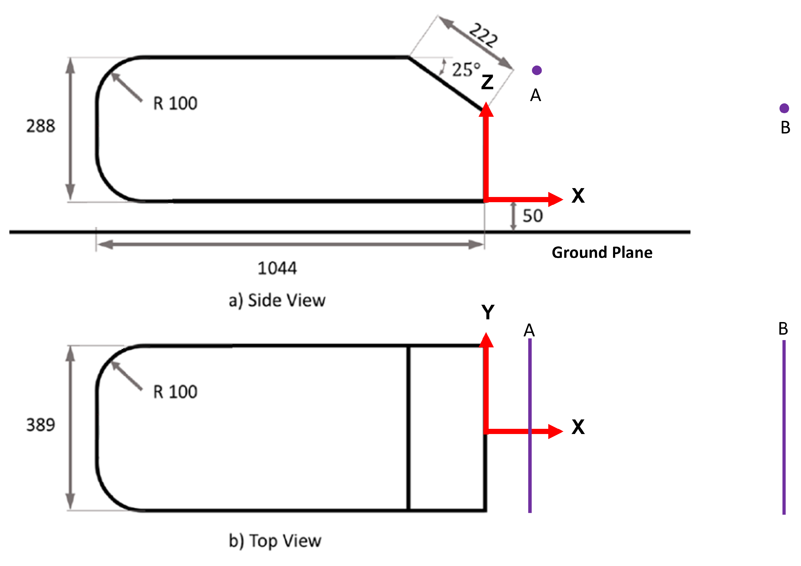
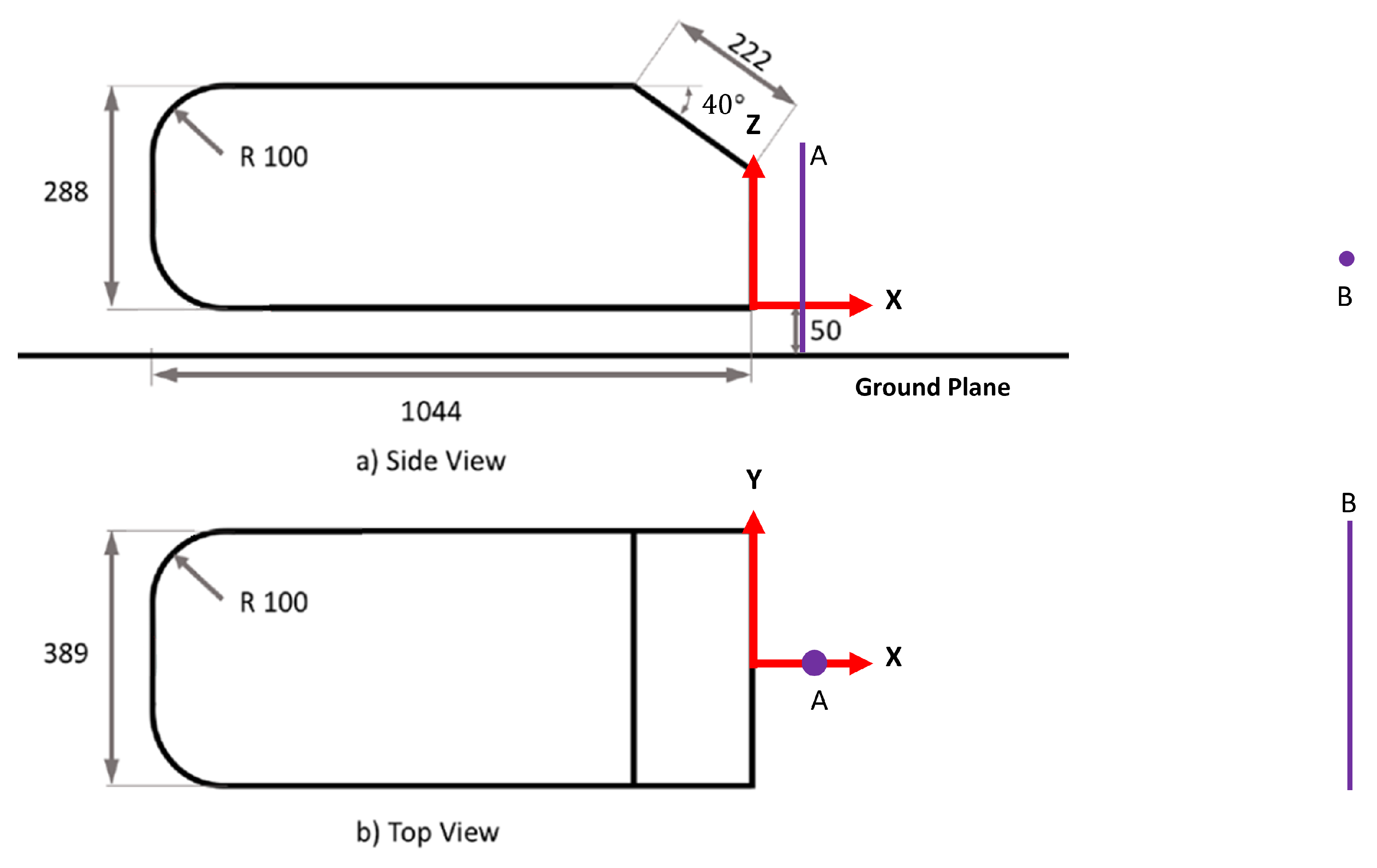
To conduct this study, two variants of the Ahmed body geometry [46] were selected: the 25-degree and the 40-degree slant-angle Ahmed body. These geometries were chosen for their ability to simplistically emulate the external aerodynamic flow of an automobile. Initially proposed by Ahmed et al. [46], the Ahmed body serves as an idealized representation of a generic vehicle shape, exhibiting all the critical features of flow past ground vehicles. It is widely regarded as the standard for validating experimental and CFD processes. The Ahmed body is a versatile model, capable of representing various automotive shapes, such as sedans, station wagons, and SUVs, by altering the frontal shapes and rear slant angles. This makes it a natural choice for our study due to the extensive computational and experimental data available in the literature, which can be used for validation; for example, see [23,24,47,48,49,50] to cite but merely a few. Its simplified yet representative geometry makes it an excellent model for studying and optimizing aerodynamic performance. This wealth of existing research ensures that our findings can be reliably compared and validated against established benchmarks, enhancing the robustness and credibility of our study. By utilizing both the 25-degree and 40-degree configurations of the Ahmed body, we aim to explore a broader range of aerodynamic behaviors. This approach provides a comprehensive analysis of the flow characteristics and the impact of turbulence model tuning on aerodynamic predictions. The Ahmed body also presents a complex enough flow problem to challenge many eddy viscosity-based turbulence models while maintaining relatively low computational costs due to its simple features. Figure 1 and Figure 2 show the dimensions, coordinate system, and reference line probes for flow validation for the 25-degree and 40-degree bodies, respectively.

Figure 1.
25-degree Ahmed body coordinate system, dimensions, and velocity probe locations. (A) U-velocity profile sampling location, (B) W-velocity profile sampling location.

Figure 2.
40-degree Ahmed body coordinate system, dimensions, and velocity probe locations. (A) U-velocity profile sampling location, (B) W-velocity profile sampling location.
A large virtual flow domain was created to reduce the effects of the domain boundary pressure reflections and blockage ratio on the final flow and force results. The length, width, and height of the domain was 15L, 4.5L, and 2.5L, respectively, with L being the length of the Ahmed body, which was used as the characteristic length for all the calculations in this work. The blockage ratio was determined to be less than 1%, which was low enough to remove almost all of the domain’s effects from the final force and moment results.
To design the mesh for the virtual wind tunnel with the vehicle model placed inside it, a commercial software, Ansa version 20.1 by Beta CAE system, was used. A hexahedral mesher was used over the entire domain and was controlled using three different volume sources, which were nested around the body to designate regions of refinement in order to properly capture the high gradient flow regimes. The refinement regions are shown in Figure 3. To resolve the near-wall flow (one of the most critical aspects of wall-bounded flows exhibiting the regions of highest shear), prism layers were used near all no-slip boundaries, with 15 layers being placed on the body and 5 layers being placed on the floor of the domain. The first layer height was 0.015 mm, and a total thickness of 3 mm was specified. This resulted in a wall node value well below 1 for all surfaces. Note that is define as , where y, , and represent the wall-normal distance of the cell centroid, the fluid kinematic viscosity, and the friction velocity, respectively; is the wall shear stress; is the fluid density; and is defined as .

Figure 3.
Mesh refinement regions.
2.2. Physics Setup
Numerical simulations of any fluid flow problem involve solutions of the Navier–Stokes (NS) equations, which are a set of conservation equations, including conservation of momentum and conservation of mass. Together, these sets of conservation equations make up the governing equations for the continuum mechanics approach to CFD simulation. The Mach number used in this work is well below 0.3, which allows for the fluid flow to be considered incompressible. The incompressible NS equations are shown using Einstein summation notation in Equations (2) and (3). In Einstein notation, a repeating index variable i implies the summation of all possible values, which in this case would be .
In the above equations (Equations (2)–(6)), , p, , and represent the instantaneous values for the velocity in the ith direction, pressure, fluid density, and the fluid viscous stress tensor, respectively. The fluid viscous stress tensor is defined as , where is the kinematic viscosity. The rate of strain tensor is shown in Equation (4). Note that in these equations and for the text to follow, upper-case symbols represent time-averaged values, and superscript primes (′) denote fluctuating values of the quantity.
The highest fidelity and most accurate form of simulation is direct numerical simulation (DNS), in which all of the scales of motion are resolved by the simulation. The computational costs of this type of simulation prove to be virtually unachievable for engineering-type flows, which in most cases are complex and have high Reynolds numbers. To solve this computational power problem, the RANS equations were developed. These equations were derived by performing Reynolds decomposition, where the time-dependent velocity, , is decomposed in a mean part, , and a fluctuating part, . The decomposed variable is then placed into the NS equations and ensemble-averaged, leading to Equations (5) and (6).
Through the method of Reynolds averaging, six new terms are introduced into the system. These new terms, , are known as the Reynolds stresses () and are shown in Equation (7). In Equation (7), is the Kronecker delta value, which is 1 when and 0 otherwise. The overbar represents averaging of the given term. The introduction of these new terms makes the once-closed NS equations now an open system of four equations and ten unknowns which is referred to as ‘the closure problem’. One of the most popular methods for closing the system of equations is that of the Boussinesq eddy viscosity hypothesis, which theorizes that the Reynolds stresses could be modeled like molecular viscous stresses.
In the equation above, k is the turbulence kinetic energy per unit mass and is defined as . One criterion of the Bousinesq hypothesis is that the momentum transfer of the turbulent flow is governed by the mixing created by the large energetic turbulent eddies. It is also assumed that the turbulent shear stress holds a linear relationship to the mean rate of strain, as observed in laminar flow and shown in Equation (7). The factor of proportionality that relates the turbulent shear stress to the mean rate of strain is called the eddy viscosity, . The eddy viscosity is a flow property defined by an algebraic function of two more flow variables, unlike the kinematic viscosity, which is a molecular property determined by the fluid. In many models, additional transport equations are introduced to solve for the eddy viscosity. The model used in this work is the SST, which is a two-equation model (introduces two transport equations) that solves transport equations for both k, the turbulent kinetic energy, and , the specific dissipation rate of turbulent kinetic energy.
The mathematical expression for the eddy viscosity, , depends on the turbulence modeling approach used. For the turbulence model, the expression for is shown in Equation (8). Other defining equations for the SST model are shown in Equations (9)–(16).
The SST default closure coefficient values are shown below in Equation (18). The following coefficients with the “1” and “2” subscripts are blended in the simulation by using Equation (16).
To implement the SST model, OpenFOAM was used, which is an open-source CFD code with a large support community. The default OpenFOAM SST was used in an incompressible flow formulation and solved by the SimpleFOAM solver. SimpleFOAM is a steady-state solution that uses the SIMPLE algorithm to handle the velocity–pressure coupling that occurs in the NS equations. Every simulation was run for at least 10,000 total iterations and averaged over the last 2000 to produce the flow field and force result data shown throughout the work.
2.3. Initial and Boundary Conditions
A freestream velocity ( of 25 m/s) was specified along the surface of the velocity inlet into the domain. Combining this freestream velocity with the characteristic length L of the body, the Reynolds number () was calculated to be , and the Mach number was found to be 0.07—well below the 0.3 threshold for the incompressible flow-solving method. These conditions match that of the experimental work of Strachen et al. [48,49], which provides the reference data for the comparisons made in this work. At the inlet to the domain, the eddy viscosity was set to 5, which equates to a turbulence intensity of 1%. The domain outlet was specified to be a pressure outlet, and the floor of the domain was given a no-slip boundary with a tangential velocity equal to that of the freestream velocity. All other boundaries of the domain were set to be zero-gradient boundaries. The Ahmed body itself was set to be a no-slip boundary to allow a boundary layer to develop over the entire body.
2.4. Design of Experiment
Five closure coefficients of the SST were varied during this work to align with those previously changed in literature (see Fu [32,33], Zhang [34], and Dangeti [35]) and are as follows: , , , , and . To efficiently explore the design space of each coefficient, the coefficients were randomly sampled from a normal distribution. This normal distribution was defined as having a standard deviation of 10% of the default values for the coefficient and a mean value that was equal to the default for the coefficient being sampled.
As previously discussed, Shapley values [10] were a precursor to many modern explainability methods and are used to calculate the marginal contribution of a player in a coalitional game. However, this does not have to strictly be a ’game’ but can also be extended to think of a model as being the game and the players as being the inputs to the model. In this manner, the contribution of an input to a model’s final output can be assessed using Equation (19)., where is the Shapley value for the input to the model, S is the coalition of model inputs without input i, F is the total number of inputs, x is the set of values for each input, and f is model function. When considering this in a modeling context, most models would need to be retrained or reformulated for every permutation of inputs, as they do not accept variable numbers of inputs. This would be an impossible task for many modeling applications, including turbulence modeling, but Lundberg et al. [11] theorized that instead of retraining the model for inputs that have been removed, the expected value for that input can be used if the features (inputs) are assumed to be independent. The expected value for coefficients in this work is simply the default value, since every coefficient has been sampled from a normal distribution centered on the default model value.
There is, however, an issue with calculating the Shapley values for large sets of inputs. This issue is that the computational cost scales with , where N is the number of features. Therefore, to calculate the Shapley values for one set of modified SST coefficients, samples (samples in this context are CFD simulations with modified coefficient sets) must be taken to generate all permutations of the modified values and default values for the coefficients. This would mean that in order to explain one set of modified coefficients for the current work, 32 simulations would need to be run with different permutations of these coefficients and the default. To reduce the computational cost, the current work introduces a parameter , defined below in Equation (20), which aims to reduce the number of required simulations per explanation.
In the above, x is the set of all variables that will be reduced, n is the total number of variables (5 in this case), and is defined below:
The parameter sums the contributions of multiple variables into one to decrease the required number of simulations. In this manner, the explanations can be produced in a one-vs- fashion, where the Shapley value is calculated for the variable of interest and . In this situation, acts as a ’background-noise’ parameter, and its Shapley values should have no trend or significant magnitude. By comparing the Shapley value of a specific coefficient to that of , we can infer the significance of the coefficient. If the Shapley value of the coefficient is not larger than that of , the coefficient is considered insignificant, as it fails to surpass the random variations of the condensed variables. Essentially, if a coefficient’s influence does not stand out against the background noise represented by , it indicates that the coefficient has little to no meaningful impact on the model’s predictions.
Figure 4 summarizes the workflow for the designed experiment. The top branches, colored in green, show the steps for using ML explainer models and SHAP to create explanations of the CFD model. The bottom branches, shown in orange, show the steps for explaining the CFD model directly using Shapley values and the one-vs- method. The center branches, shown in blue, describe the common steps between both methods.
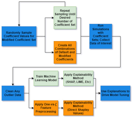
Figure 4.
Workflow diagram of the designed experiment. Blue branches: common workflow steps. Green branches: steps for the machine learning explainer model explanations. Orange branches: steps for the direct Shapley value explanation method.
3. Results and Discussion
3.1. Mesh Independence
First, a mesh independence study was performed for both the 25- and 40-degree Ahmed bodies. A starting mesh was created for each body using a base size that controlled the cell size nearest the body and scaled the volume sources, which were used away from the body. This base mesh is called the coarse mesh, and a medium and a fine mesh were created by reducing the base size by 2 and 4, respectively. All the simulations were run until they converged and then averaged over the last 2000 iterations. The differential lift and drag coefficients for each simulation with respect to the experimental values of Stracahn [48] are shown in Table 1. In the table, it is seen that for both bodies, a mesh independence is achieved between the medium and fine meshes. For computational efficiency, the medium mesh was chosen for both bodies to conduct the rest of the simulations in this work.

Table 1.
Differential force coefficient versus mesh sizing for different Ahmed body angle configurations.
3.2. Application of Shapley Values to Force Coefficient Predictions
Once the medium mesh was chosen, the coefficient was selected to be explained using Shapley values, and the other closure coefficients were condensed into the parameter. It is important to stop and note that the closure coefficients that are condensed into are not condensed during the actual running of the simulation but only during the explanation portion of the analysis. A random set of coefficients was generated according to the method listed in the previous section and then simulated in CFD. The given permutations of the default and modified coefficients were created and simulated. These simulations (four total for each set of modified coefficients) were then used to generate Shapley values for the original set of modified coefficients. This process was repeated 9 times, which required a total of 27 simulations (9 for the modified coefficient sets shown in Table 2, and 18 for the permutations), plus the default results. The resulting Shapley values explain the marginal contributions of and towards the lift and drag predictions of the model.

Table 2.
Modified coefficient sets for testing Shapley values as an explainability method for the 25-degree Ahmed body.
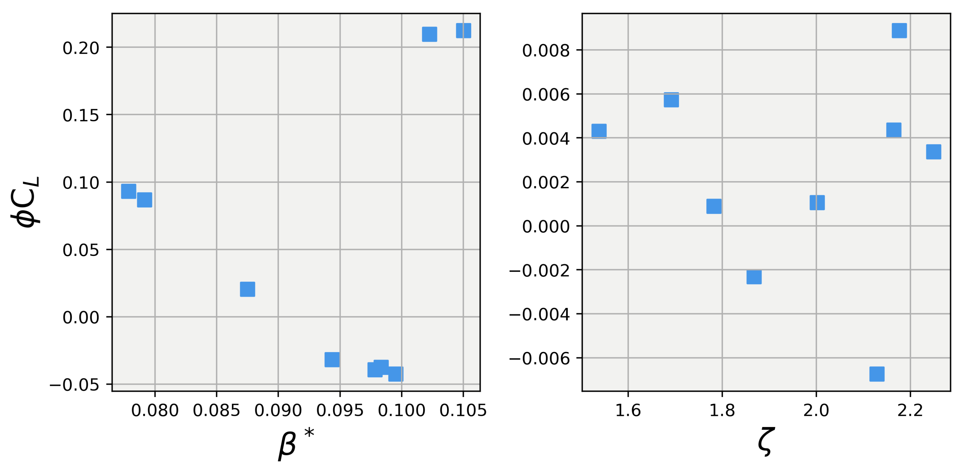
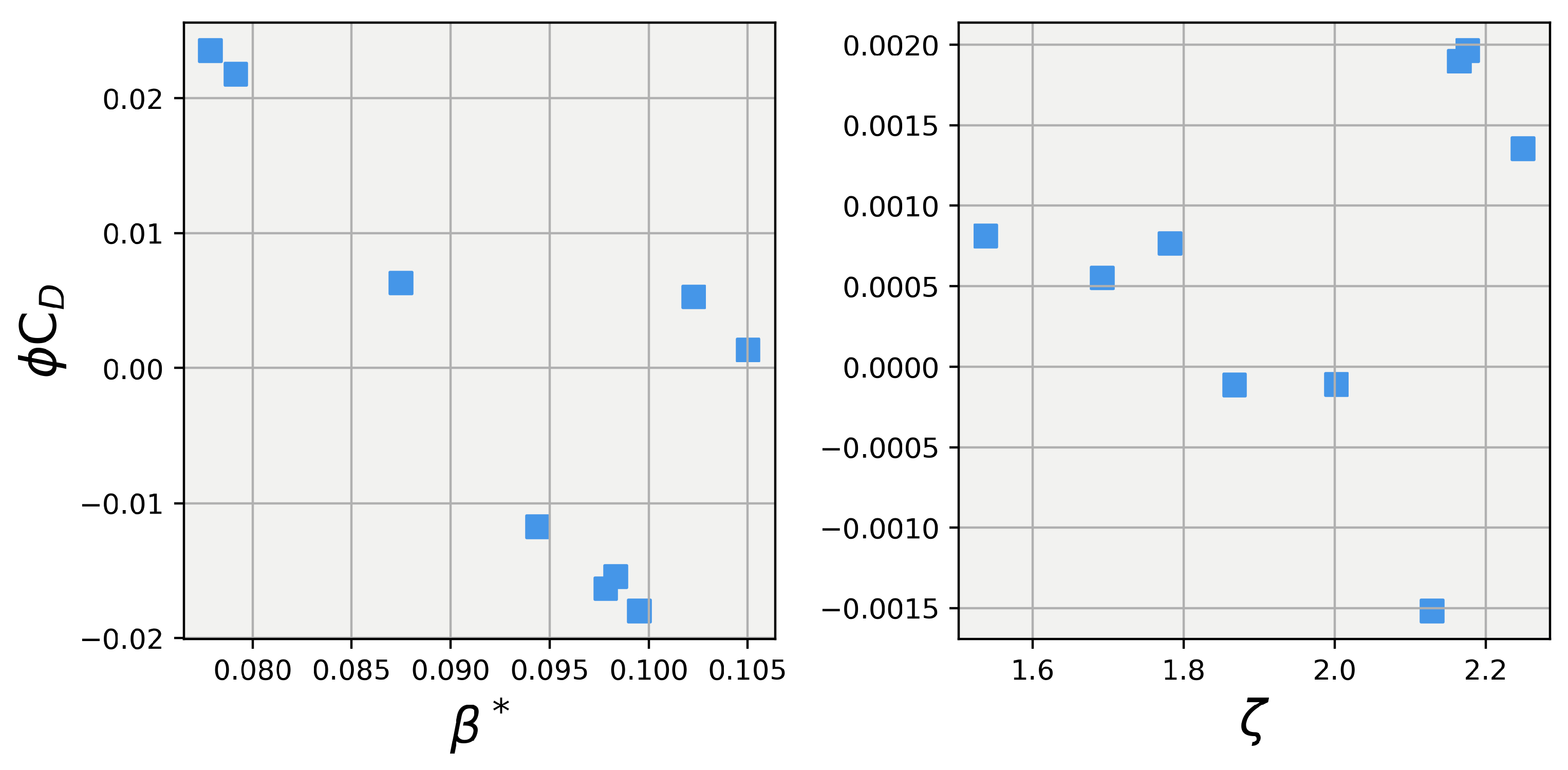
For each of the simulations performed, the forces were averaged over the last 2000 iterations, converted to lift and drag coefficients, and are shown in Table 3. Note that the force coefficient is defined as , where denotes force in x direction and A is the characteristic area. It clear from the table that some sets of coefficients improve the predicted lift and drag values to be in closer alignment with the reference experimental values from Stratchan [49]. However, what the table is not able to show is what role played in the change in predictions and what roles the other coefficients played. To explain how the coefficients affected the results, the Shapley values were calculated for and and are shown in Figure 5 and Figure 6.

Table 3.
Average delta force coefficient results for the six sample coefficient sets compared to the 25-degree Ahmed body experimental work of Strachan [49].

Figure 5.
Explanations of lift coefficient prediction contributions from and using Shapley values. Left: Shapley value for vs. ; Right: Shapley value for vs. .

Figure 6.
Explanations of prediction contributions from and using Shapley values. Left: Shapley value for vs. ; Right: Shapley value for vs. .
Figure 5 and Figure 6 illustrate the marginal contribution of each coefficient to the total output (predicted lift or drag) of the CFD model. Unlike traditional Shapley value calculations, which assume that the baseline case (when no players participate) yields an output of zero, these Shapley values assume that the baseline case is represented by the output from the default coefficients of the SST model. By using the default coefficients as the baseline, these plots reveal the marginal contributions of each coefficient in terms of the deviation from the default prediction. This approach provides a clearer understanding of how each coefficient influences the changes in the predicted lift and drag compared to the default model.
Examining the left pane of Figure 5 shows a clear linearly decreasing trend in lift as is increased from its lowest values up to about 0.098. After is increased past approximately 0.098, a sharp jump in lift occurs and holds at a relatively constant value for values above this threshold. The right pane of Figure 5 shows a very different result in which no discernible trend occurs between and the lift coefficient. This result is inline with the expected outcome, because is the collection of all of the marginal lift contributions from the four other closure coefficients, which, as mentioned previously, makes it analogous to a background noise parameter. Therefore, it is fair to say that a coefficient can be said to be influential on the output of the model if it shows a stronger trend and magnitude than the parameter to which it is compared. For this study, can be said to hold a strong influence over the simulation, as it has a far greater magnitude and trend than those of .
Analyzing the data shown in Figure 6 reveals that the trends seen in the Shapley values for carry into the drag coefficient values. shows the same linear dependence on , with a sharp up-kick around = 0.098, while has no significant trend in magnitude.
To further test the viability of Shapley values as explanations, was chosen to be removed from the parameter. This was done because it was seen to be one of the more influential parameters in the prediction of lift and drag for the Gen-6 NASCAR Cup car studied in the work of Fu et al. [32,33]. The process of sampling values was repeated according to the procedure previously discussed, but because is going to be analyzed directly, the required permutations increased to eight simulations per explanation. In light of the limited computational power of this study, the number of coefficient sets that could be sampled was only 3, creating a total of 21 simulations: 3 modified coefficient sets and 18 permutations.
Figure 7 and Figure 8 show the Shapley values for lift and drag, respectively, for the , , and . The first thing to note is that the explanations for for both lift and drag stayed the same, which is expected, since the contributions of were already accounted for in the first set of simulations. In the first set, the explanations of were combined into , and their effects were taken into account when calculating the explanations for the s. When analyzing the explanations for in Figure 5, one can observe that played a small role in the prediction of lift, while , in general, had a higher magnitude of influence. When observing the drag values in Figure 8, almost the same observation can be made for , with it contributing very little to the overall drag prediction. However, in this case, also played almost no role, with its maximum contribution being less than three counts (a count being defined as a dimensionless force/moment coefficient value of 0.001).
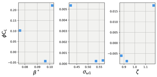
Figure 7.
Explanations of prediction contributions from , , and using Shapley values.
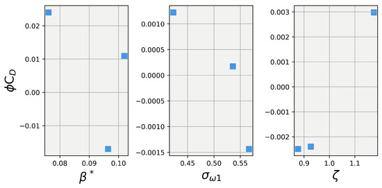
Figure 8.
Explanations of prediction contributions from , , and using Shapley values.
While the plots in Figure 7 and Figure 8 do not reveal a large amount of information about the trends of the coefficients (other than their relative magnitude of influence), they do highlight another interesting observation about the Shapley value explanation method. Since the explanations for did not change when was removed from , it would actually be a more efficient sampling method to repeat the one-vs-rest method for and simply include into . This becomes especially true as the user wishes to increase the number of closure coefficients analyzed, since the number of simulations per explanation grows as , where N is the number of coefficients that the user wishes to directly explain. However, when analyzing the per-explanation cost of the one-vs-rest sampling method, a constant cost of is found, since .
3.3. Application of Machine Learning Explainer Models and SHAP to Force Coefficient Predictions
The process of repeatedly removing coefficients from could be continued until all of the closure coefficients were directly explained by the Shapley values method, eliminating the need for . However, as already discussed, the sampling cost for the direct calculation of Shapley values increases quite significantly with every variable that is to be explained. This sampling cost must be considered even more heavily when applying this method to non-simplified geometries where the simulation time is on the order of days and not hours like those needed for the current study. For such situations, it is crucial to develop a method that can provide clear and accurate explanations using the fewest possible simulations. This approach not only saves computational resources and time but also enhances the efficiency and practicality of the analysis. By minimizing the number of required simulations, researchers can more rapidly and effectively understand the underlying dynamics and improve model predictions. Subsequently, in the present work, these explainer models will be trained using the turbulence model closure coefficients used in the CFD simulations as features and the CFD force coefficient predictions as targets. The ML model predictions for lift and drag can then be explained using ML explainability methods, such as SHAP, for a fraction of the cost of explaining the CFD simulation, since a prediction from the ML model only takes seconds.
Using explainer models in this manner also lays the groundwork for addressing more complex problems where data can be sampled to acquire features and targets, but the features cannot be directly manipulated to create the sampling permutations required for performing Shapley value explanations. For instance, consider a scenario where we aim to explain the contributions of experimental measurements of pressure and velocity to boundary layer thickness, . In this case, we want to understand how pressure and velocity impact the boundary layer thickness predictions. To make these explanations using Shapley values for a specific sample [, , ], we would need to manipulate the pressure and velocity into four different permutations, as shown in Table 4. However, this manipulation of pressure and velocity may not be feasible, depending on the experimental setup, which can prevent the use of Shapley values for explanation. This limitation underscores the importance of developing methods that can work with existing data constraints. By leveraging explainer models, we can provide valuable insights, even in situations where traditional methods fall short due to their inability to manipulate experimental conditions directly.

Table 4.
Example of infeasible permutations required to explain experimental measurements.
To generate the training data needed for the ML explainer models, additional sampling of closure coefficients was performed using the previously described method for creating the modified coefficient sets for the Shapley value method. The final sizes of the training datasets were 77 and 50 for the 25-degree body and 40-degree body, respectively. Each dataset was preprocessed by manually removing any outlier data that were seen to be non-physical. The features for the models were the five closure coefficients, and the targets were the lift and drag coefficients obtained from the CFD simulations. The Scikit-learn [51] Python library (version 1.3.2), a collection of validated open-source ML training tools and models, was used to develop the models and training sequences. For each of the models trained, a hyperparameter tuning search was conducted to optimize the model’s performance for the specific geometry and target (lift or drag). To ensure that the model’s performance was generalizable and not merely memorizing the training data, a 10-iteration shuffle split cross-validation method was employed [52]. During each iteration of the shuffle split, a set of hyperparameters was chosen for the model, and the data were randomly divided into training and testing subsets. The model was then fit on the training set and evaluated on the testing set. This procedure was repeated for 10 iterations, and the set of hyperparameters with the best average testing performance was selected. The model’s performance was evaluated by comparing the training and testing scores for each iteration. If the model performed significantly better on the training set than on the testing set, overfitting had occurred. Overfitting happens when the model simply memorizes the training data, leading to poor performance on new data. Conversely, if the model had both low training and testing scores, underfitting had occurred. Underfitting indicates that the model lacks the complexity to fully capture the underlying trends in the data, necessitating the use of a more complex model.
The training process began with the 25-degree Ahmed body case. Five commonly used regression models were trained: ridge [53], random forest [54], XGBoost (XGB) [55], support vector machine (SVM) [56], and K-nearest neighbors (KNN) [57]. A word of caution here: these models were selected to evaluate the performance of various types of models on the relatively small dataset used in this study, which has the potential of adversely skewing the results, as we will see later. During training, one of the first observations was a significant decrease in model performance across all types when a newly generated set of data was introduced. After thorough investigation, it was discovered that an incorrect parameter set during the training process had generated perfectly correlated sets of closure coefficients for testing. This perfect correlation caused the five closure coefficients to essentially represent the information of only one feature, but with the complexity and cost of five. Consequently, the models struggled to train effectively due to the lack of diverse information, resulting in lower average testing scores and an increased tendency to overfit. This error, though easily resolved, underscores a crucial principle in machine learning: highly correlated features should generally be removed, especially when working with small datasets. This is particularly important in our study for two main reasons. First, small datasets make the model highly sensitive to the quality of the data. Second, CFD simulation sampling is costly, making it essential to convey as much information as possible for each sample. Ensuring the dataset is free from highly correlated features can improve the model’s performance by providing diverse and relevant information for training. This approach not only enhances the robustness of the model but also maximizes the value derived from each costly CFD simulation sample.
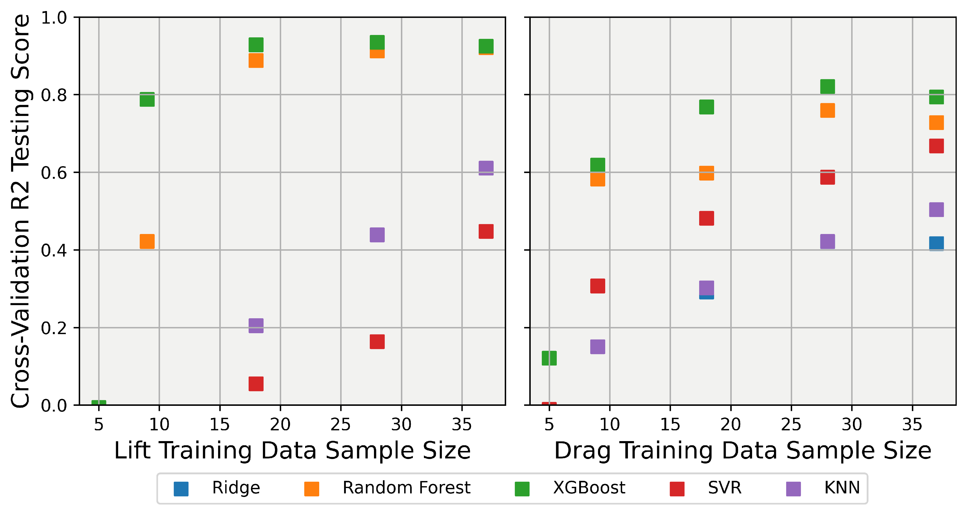
One of the goals of this work was to identify ML models that are efficient at fitting the data using a small number of samples, saving valuable CFD computation time. To test which of the models performed best at capturing the trend ointhe CFD data with minimal training samples, each of the models was trained with cross-validation using reduced training sample sizes of 80%, 60%, 40%, 20%, and 10%. The results for each of the models are shown in Figure 9, with the testing R-squared score shown on the y-axis and the number of samples used to train the model shown on the x-axis. Examining the testing scores shows that none of the models could provide accurate results below a sample size of approximately 10, with the testing scores becoming so poor below this sample number that the figure was clipped at 0 to keep the figure scaling neat. At the upper end of the training samples, XGB and random forest were seen to be the best, with SVR and KNN performing similarly to each other, and ridge performing the worst of all the models.
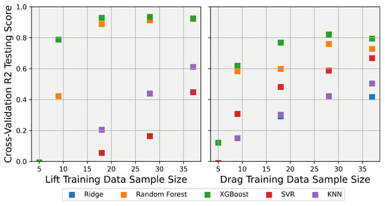
Figure 9.
Dependence of R-squared score on the size of training data for the 25-degree Ahmed Body explainer models. Left: Scores for for prediction; Right: Scores for for prediction (note that the y-axis is clipped at 0).
All of the data were then used to train the model during the cross-validation phase. The results are shown in Table 5. The metrics displayed in Table 5 are the R-squared score and the mean absolute error (MAE). The R-squared score is defined in Equation (22), where y is the true value, is the predicted value, is the mean of the true values, and n is the number of samples. The results from the table support what was seen in the restricted training size study, with XGB and random forest performing the best, followed by a close tie between SVM and KNN.

Table 5.
Cross-validation scores for ML models predicting lift and drag for the 25-degree Ahmed body.
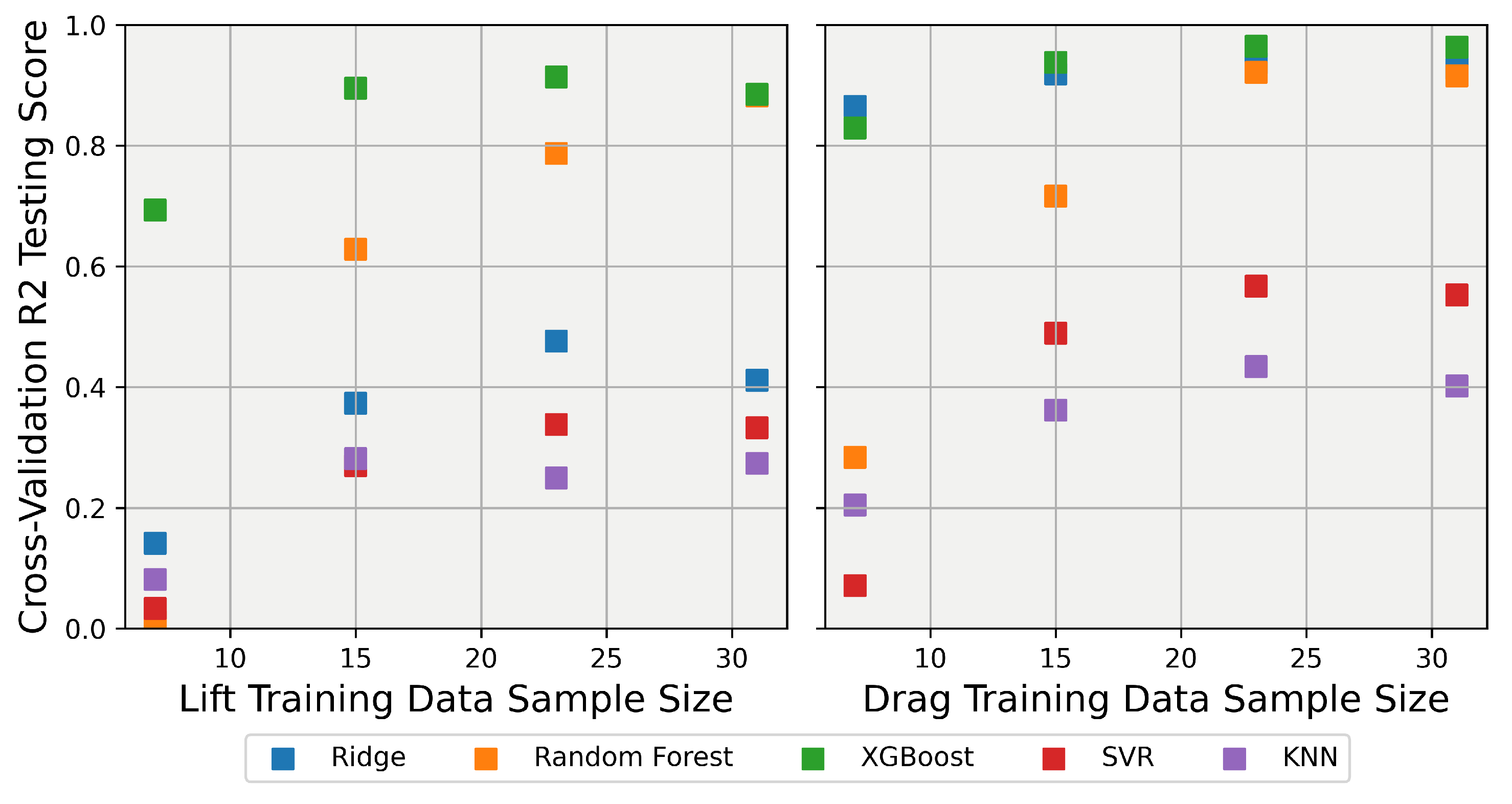
Moving to the 40-degree body, explainer models for the lift and drag coefficients were developed according to the same procedure as the 25-degree body. The cross-validation scores for each model were calculated and are listed in Table 6. For the 40-degree body, predicting the lift coefficient proved to be the most challenging, with only the random forest and XGB models able to achieve an R-squared score higher than 0.80. In contrast, predicting the drag coefficient was easier for the models, with the ridge, XGB, and random forest models achieving very high R-squared score, while KNN was the worst predictor. Each model was then tested using varying training data sizes to assess how well they would adapt to smaller datasets. The results for the 40-degree training size variation are shown in Figure 10. Clearly, as can be seen in Figure 10 (left), for lift prediction, the XGB model had the best prediction capability by a wide margin for most of the sample sizes. Although it outperformed the other models for sample sizes below 10, it still struggled to make adequate predictions. Turning to the drag predictions shown in the right panel of Figure 10, it is evident that the ridge, XGB, and random forest models maintained adequate performances, even at sample sizes lower than 10 samples. These results suggest that while some models, like XGB, excel in predicting specific aerodynamic characteristics with limited data, others, such as ridge and random forest, offer robust performance across various sample sizes. By analyzing the performance of these models, we can better understand their strengths and limitations, ultimately guiding the selection of the most appropriate model for specific aerodynamic prediction tasks.

Table 6.
Cross-validation scores for ML models predicting lift and drag for the 40-degree Ahmed body.
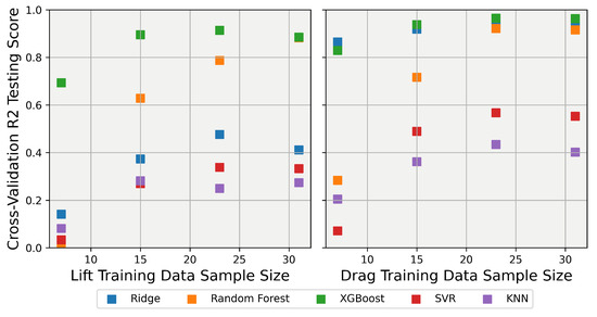
Figure 10.
Dependence of R-squared score on the size of training data for the 40-degree Ahmed Body explainer models. Left: Scores for for prediction; Right: Scores for for prediction (note the y-axis is clipped at 0).
Taking all factors into account, the XGB and random forest models for the 25-degree body and the random forest model for the 40-degree body were selected to have their predictions explained using SHAP. It is important to note that both the XGB model and the random forest model belong to the “tree model” category. Although they are expected to present relatively similar explanations, they are not identical. The XGB model is a more advanced form of tree modeling, which may leverage the features in different ways. The SHAP values for the 25-degree body were calculated for each closure coefficient and are plotted in Figure 11 and Figure 12. Both models agree that has the greatest influence on the lift prediction and show almost identical trends, with the random forest model differing slightly within the range of . When examining the SHAP values for the other coefficients, it becomes evident that the models do not fully agree on the importance of each coefficient. The XGB model appears to have utilized a different form of feature selection during its tree creation, allowing for more influence from all features. In contrast, the random forest model assigned very little influence to these features. Despite these differences in trends for the other four coefficients, the overall magnitudes are quite similar for both models, with most of the coefficients having an influence centered around 0 for the majority of the data points. By analyzing these SHAP values, we can gain insights into how each model interprets the importance of different features, helping to understand the strengths and limitations of each model in predicting lift for the 25-degree body.
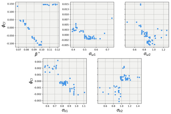
Figure 11.
SHAP values for predictions obtained using the XGBoost regression model on the 25-degree Ahmed body.

Figure 12.
SHAP values for predictions obtained using the random forest regression model on the 25-degree Ahmed body.
Figure 13 and Figure 14 show the SHAP values for the predictions obtained using the random forest regression model on the 25-degree Ahmed body, respectively. Once again, the explanations for the two models largely align for the closure coefficient but deviate between . It appears that in this area, the XGB models do a much better job of smoothly learning from the training data, while the random forest struggles to find a manner to smoothly split the data for predictions; an issue that could be solved for the random forest model with more tuning. The XGB and random forest models give largely the same bulk magnitude of influence to the other four closure coefficients but differ in the trend, with the random forest having mostly ignored the features, while XGB leveraged the features and was able to show their effects on the prediction.
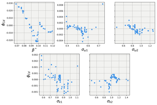
Figure 13.
SHAP values for predictions obtained using the XGBoost regression model on the the 25-degree Ahmed body.
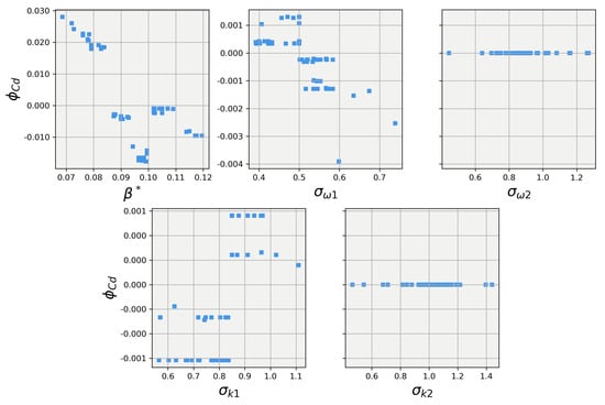
Figure 14.
SHAP values for predictions obtained using the random forest regression model on the the 25-degree Ahmed body.
Turning our attention to the results of the 40-degree body explainer models, Figure 15 and Figure 16 show the results of the SHAP value calculations for the 40-degree body. The first observation is that while has the dominant influence over the lift and drag predictions, it takes a much more non-linear trend compared to the 25-degree body. Secondly, while small, the random forest for the 25-degree body did show the other four closure coefficients having some influence on the lift and drag predictions. However, the 40-degree explainer models show that for both lift and drag, the four other closure coefficients had little to no influence on the lift and drag predictions. This difference in influence aligns well with Pope’s [31] conjecture that the closure coefficients are not a universal set for all applications but are dynamic and must be tuned, albeit according to constrained relationships, for each particular application.
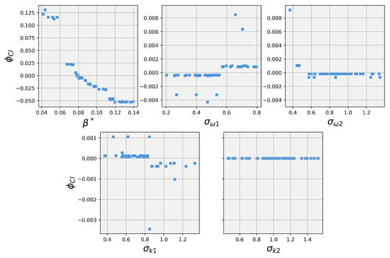
Figure 15.
SHAP values for predictions obtained using the random forest regression model on the the 40-degree Ahmed body.
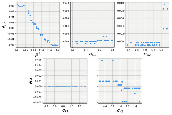
Figure 16.
SHAP values for predictions obtained using the random forest regression model on the the 40-degree Ahmed body.
The explainer models for the 25-degree body were used, along with the SHAP explanations, to generate a set of estimated optimal coefficients. Based on the SHAP explanations, it can be seen that decreasing leads to increasing lift coefficients; however, following the trends made the optimal exist at the edge of the predictive range for the models where the prediction strength was weak. An iterative process was used, where a set of coefficients would be generated by the ML model and tested in CFD. If the value was not close enough to the optimal value, due to being at the edge of the model’s prediction limits, the CFD data samples would then be added back into the model training set. New predictions would then made be using the updated model until the optimal set of CFD closure coefficients was achieved. The results of this process are shown in Table 7, where it is seen that the improved set of coefficients vastly improves the CFD simulation’s predictive capability for lift and drag. The same process was repeated for the 40-degree body, and the results are shown in Table 8. The 40-degree body saw a smaller reduction in error, as the baseline was effective at predicting the coefficients, but the optimal set of coefficients was able to almost perfectly align with the experimental results, with the largest error between lift and drag being only −0.34%.

Table 7.
Force results for the improved set of closure coefficients for the 25-degree Ahmed body.

Table 8.
Force results for the improved set of closure coefficients for the 40-degree Ahmed body.
In tuning these coefficient sets, it is import to remember that while even though they were set in a rather ad hoc manner, they were still set in such a way as to adhere to the physical principles shown in experimental works. First, analyzing the limits on , this coefficient was determined by Wilcox [58] using experimental data on decaying homogeneous isotropic turbulence (HIT). In the HIT regime, turbulent kinetic energy (TKE) is seen to follow the relationship of , where n is known as the decay exponent and is defined as . The value for n is a much-debated topic, with Townsend [59] originally proposing , but modern experimental works on isotropic and homogeneous–anisotropic turbulence show a range of [60,61]. There has even been some computational work on the subject from Taghizadeh et al. [62], where they found a range of . When considering the influence that n has on , this leads to a debated range of of approximately 15–30% compared to the default value. The current work restricts variance to 10%, which is well within the debated range and close to Townsend’s original proposition.
4. Conclusions
This paper demonstrated the efficacy of ML and explainability tools in the CFD workflow by tuning the closure coefficients of a RANS turbulence model to optimal values. Specifically, the SST turbulence model’s closure coefficients were optimized for two variants of the idealized ground vehicle model known as the Ahmed body. Shapley values were used to directly explain CFD predictions, proving accurate but costly. Explainer ML models, trained on CFD simulation data, provided a more efficient way to explain the effects of closure coefficients on CFD outputs. The SHAP technique was applied to these models, elucidating the relationships between closure coefficients and CFD force predictions. This approach reduced force prediction errors to less than 7% and 0.5% for the 25-degree and 40-degree slant-angle Ahmed bodies, respectively. Some key conclusions to highlight are as follows:
- Shapley values present a way to create explanations directly on the CFD model itself, but they have a high sampling cost. They are seen to be able to describe the complex interactions that occur when simultaneously varying all closure coefficients.
- A one-vs-rest Shapley value method in which a sub-variable was introduced was observed to be the most efficient way of reducing the high sampling cost of the Shapley method. This method reduce the per-explanation cost from , where N is the total number of inputs to be explained, to a constant cost of four simulations per explanation, since .
- Explainer models proved to be a computationally efficient way to sample the domain space for the creation of input/output relationships for CFD simulations. It was seen that of the types of explainer models tested, including the random forest and the XGB models, proved to be best for this application due to their good balance of performance on the data needed for training.
- The SHAP method of explanation was seen to be able to create explanations for the force predictions of the CFD.
- The optimal closure coefficients for the 25-degree Ahmed body differed from that of the 40-degree Ahmed body. This demonstrates the strength of this method compared to traditional CFD tuning methods, as it was able to generate distinctly optimal coefficients for different geometries. The result also aligns with the hypothesis of Pope [31], that these coefficients are not universal, but instead, they exist within a range that may need to be modified for different applications.
One of the limitations of this work is that it focused on the application of ML and explainability in the optimization of CFD closure coefficients, specifically for predicting aerodynamic force coefficients. However, this is just the beginning, as the potential of these techniques extends far beyond this initial application. By concentrating on aerodynamic force coefficients, we have established a foundation for tackling more complex problems. In future research, we aim to broaden the scope of ML tools for CFD by conducting similar analyses that focus on the flow field, particularly in the wake region, as the target. This extension will allow us to explore the detailed flow dynamics and gain deeper insights into the behavior of turbulence and wake structures. By shifting the focus from force coefficients to flow field characteristics, we hope to uncover new opportunities for optimizing aerodynamic performance and enhancing the fidelity of turbulence models. The authors hope that this work will encourage other researchers to explore the creation of CFD process tools using ML and explainability as methods of optimizing current CFD processes and laying the groundwork for future ML and CFD modeling.
Author Contributions
Conceptualization, C.P.B. and M.U.; methodology, C.P.B., S.D. and M.U.; software, C.P.B. and S.D.; validation, C.P.B., S.D. and M.U.; formal analysis, C.P.B., S.D. and M.U.; investigation, C.P.B., S.D. and M.U.; resources, M.U.; data curation, C.P.B. and S.D.; writing—original draft preparation, C.P.B.; writing—review and editing, C.P.B. and M.U.; visualization, C.P.B. and S.D.; supervision, M.U.; project administration, M.U.; funding acquisition, M.U. All authors have read and agreed to the published version of the manuscript.
Funding
Charles Patrick Bounds was supported by the National Science Foundation (NSF) Graduate Research Fellowship Program (GRFP) during the execution of this project.
Data Availability Statement
The original contributions presented in the study are included in the article, further inquiries can be directed to the corresponding author.
Acknowledgments
The authors acknowledge Charlotte’s MOSAIC Computing and University Research Computing (URC) teams for their invaluable computational support. Their assistance and resources were crucial to the successful completion of this research. We deeply appreciate their expertise and dedication. The authors would also like to acknowledge Jordan Davis for her supporting role in proofreading and editing this work.
Conflicts of Interest
The authors declare no conflicts of interest.
Abbreviations
The following abbreviations are used in this manuscript:
| AI | Artifical intellegence |
| CFD | Computational fluid dynamics |
| LIME | Local interpretable model–agnostic explanations |
| ML | Machine learning |
| RANS | Reynolds-averaged Navier–Stokes |
| SHAP | Shapley additive explanations |
| SIMPLE | Semi-implicit method for pressure-linked Equations |
References
- Education, I.C. What Is Machine Learning? 2020. Available online: https://www.ibm.com/cloud/learn/machine-learning (accessed on 14 September 2022).
- Doshi-Velez, F.; Kim, B. Towards a rigorous science of interpretable machine learning. arXiv 2017, arXiv:1702.08608. [Google Scholar]
- Molnar, C.; Casalicchio, G.; Bischl, B. Interpretable machine learning—A brief history, state-of-the-art and challenges. In Proceedings of the Joint European Conference on Machine Learning and Knowledge Discovery in Databases, Ghent, Belgium, 14–18 September 2020; Springer: Berlin/Heidelberg, Germany, 2020; pp. 417–431. [Google Scholar]
- Guidotti, R.; Monreale, A.; Ruggieri, S.; Turini, F.; Giannotti, F.; Pedreschi, D. A survey of methods for explaining black box models. ACM Comput. Surv. (CSUR) 2018, 51, 1–42. [Google Scholar] [CrossRef]
- Ribeiro, M.T.; Singh, S.; Guestrin, C. Model-agnostic interpretability of machine learning. arXiv 2016, arXiv:1606.05386. [Google Scholar]
- Ribeiro, M.T.; Singh, S.; Guestrin, C. “Why should I trust you?” Explaining the predictions of any classifier. In Proceedings of the 22nd ACM SIGKDD International Conference on Knowledge Discovery and Data Mining, San Francisco, CA, USA, 13–17 August 2016; pp. 1135–1144. [Google Scholar]
- Štrumbelj, E.; Kononenko, I.; Šikonja, M.R. Explaining instance classifications with interactions of subsets of feature values. Data Knowl. Eng. 2009, 68, 886–904. [Google Scholar] [CrossRef]
- Štrumbelj, E.; Kononenko, I. An efficient explanation of individual classifications using game theory. J. Mach. Learn. Res. 2010, 11, 1–18. [Google Scholar]
- Štrumbelj, E.; Kononenko, I. Explaining prediction models and individual predictions with feature contributions. Knowl. Inf. Syst. 2014, 41, 647–665. [Google Scholar] [CrossRef]
- Shapley, L. Quota Solutions op n-person Games. In Contributions to the Theory of Games (AM-28), Volume II; Kuhn, H.W., Tucker, A.W., Eds.; Princeton University Press: Princeton, NJ, USA, 1953; pp. 343–360. [Google Scholar]
- Lundberg, S.M.; Lee, S.I. A unified approach to interpreting model predictions. Adv. Neural Inf. Process. Syst. 2017, 30, 4768–4777. [Google Scholar]
- Lundberg, S.M.; Erion, G.; Chen, H.; DeGrave, A.; Prutkin, J.M.; Nair, B.; Katz, R.; Himmelfarb, J.; Bansal, N.; Lee, S.I. From local explanations to global understanding with explainable AI for trees. Nat. Mach. Intell. 2020, 2, 56–67. [Google Scholar] [CrossRef] [PubMed]
- Shrikumar, A.; Greenside, P.; Kundaje, A. Learning important features through propagating activation differences. In Proceedings of the International Conference on Machine Learning (PMLR), Sydney, Australia, 6–11 August 2017; pp. 3145–3153. [Google Scholar]
- Ling, J.; Kurzawski, A.; Templeton, J. Reynolds averaged turbulence modelling using deep neural networks with embedded invariance. J. Fluid Mech. 2016, 807, 155–166. [Google Scholar] [CrossRef]
- Wu, J.L.; Xiao, H.; Paterson, E. Physics-informed machine learning approach for augmenting turbulence models: A comprehensive framework. Phys. Rev. Fluids 2018, 3, 074602. [Google Scholar] [CrossRef]
- Wang, J.X.; Wu, J.L.; Xiao, H. Physics-informed machine learning approach for reconstructing Reynolds stress modeling discrepancies based on DNS data. Phys. Rev. Fluids 2017, 2, 034603. [Google Scholar] [CrossRef]
- Jiang, C.; Vinuesa, R.; Chen, R.; Mi, J.; Laima, S.; Li, H. An interpretable framework of data-driven turbulence modeling using deep neural networks. Phys. Fluids 2021, 33, 055133. [Google Scholar] [CrossRef]
- McConkey, R.; Yee, E.; Lien, F.S. Deep structured neural networks for turbulence closure modeling. Phys. Fluids 2022, 34, 035110. [Google Scholar] [CrossRef]
- Bar-Sinai, Y.; Hoyer, S.; Hickey, J.; Brenner, M.P. Learning data-driven discretizations for partial differential equations. Proc. Natl. Acad. Sci. USA 2019, 116, 15344–15349. [Google Scholar] [CrossRef]
- Stevens, B.; Colonius, T. FiniteNet: A fully convolutional LSTM network architecture for time-dependent partial differential equations. arXiv 2020, arXiv:2002.03014. [Google Scholar]
- Shan, T.; Tang, W.; Dang, X.; Li, M.; Yang, F.; Xu, S.; Wu, J. Study on a fast solver for Poisson’s equation based on deep learning technique. IEEE Trans. Antennas Propag. 2020, 68, 6725–6733. [Google Scholar] [CrossRef]
- Zhang, Z.; Zhang, L.; Sun, Z.; Erickson, N.; From, R.; Fan, J. Solving Poisson’s Equation using Deep Learning in Particle Simulation of PN Junction. In Proceedings of the 2019 Joint International Symposium on Electromagnetic Compatibility, Sapporo and Asia-Pacific International Symposium on Electromagnetic Compatibility (EMC Sapporo/APEMC), Sapporo, Japan, 3–7 June 2019; IEEE: Piscataway, NJ, USA, 2019; pp. 305–308. [Google Scholar]
- Ashton, N.; Revell, A. Comparison of RANS and DES Methods for the DrivAer Automotive Body; Technical Report, SAE Technical Paper; SAE: Warrendale, PA, USA, 2015. [Google Scholar]
- Ashton, N.; West, A.; Lardeau, S.; Revell, A. Assessment of RANS and DES methods for realistic automotive models. Comput. Fluids 2016, 128, 1–15. [Google Scholar] [CrossRef]
- Misar, A.S.; Bounds, C.; Ahani, H.; Zafar, M.U.; Uddin, M. On the Effects of Parallelization on the Flow Prediction around a Fastback DrivAer Model at Different Attitudes; Technical Report, SAE Technical Paper; SAE: Warrendale, PA, USA, 2021. [Google Scholar]
- Slotnick, J.P.; Khodadoust, A.; Alonso, J.; Darmofal, D.; Gropp, W.; Lurie, E.; Mavriplis, D.J. CFD Vision 2030 Study: A Path to Revolutionary Computational Aerosciences; Technical Report NASA/CR–2014-218178; National Aeronautics and Space Administration (NASA): Washington, DC, USA, 2014.
- Frey Marioni, Y.; de Toledo Ortiz, E.A.; Cassinelli, A.; Montomoli, F.; Adami, P.; Vazquez, R. A machine learning approach to improve turbulence modelling from DNS data using neural networks. Int. J. Turbomachinery Propuls. Power 2021, 6, 17. [Google Scholar] [CrossRef]
- Zhu, L.; Zhang, W.; Kou, J.; Liu, Y. Machine learning methods for turbulence modeling in subsonic flows around airfoils. Phys. Fluids 2019, 31, 015105. [Google Scholar] [CrossRef]
- Beetham, S.; Capecelatro, J. Formulating turbulence closures using sparse regression with embedded form invariance. Phys. Rev. Fluids 2020, 5, 084611. [Google Scholar] [CrossRef]
- Liu, W.; Fang, J.; Rolfo, S.; Moulinec, C.; Emerson, D.R. An iterative machine-learning framework for RANS turbulence modeling. Int. J. Heat Fluid Flow 2021, 90, 108822. [Google Scholar] [CrossRef]
- Pope, S. A Perspective on Turbulence Modeling. In Modeling Complex Turbulent Flows; Springer: Dordrecht, The Netherlands, 1999. [Google Scholar]
- Fu, C.; Uddin, M.; Robinson, C.; Guzman, A.; Bailey, D. Turbulence models and model closure coefficients sensitivity of NASCAR Racecar RANS CFD aerodynamic predictions. SAE Int. J. Passeng.-Cars-Mech. Syst. 2017, 10, 330–345. [Google Scholar] [CrossRef]
- Fu, C.; Bounds, C.; Uddin, M.; Selent, C. Fine Tuning the SST k-ω Turbulence Model Closure Coefficients for Improved NASCAR Cup Racecar Aerodynamic Predictions. SAE Int. J. Adv. Curr. Pract. Mobil. 2019, 1, 1226–1232. [Google Scholar] [CrossRef]
- Zhang, C.; Uddin, M.; Selent, C. On Fine Tuning the SST K–ω Turbulence Model Closure Coefficients for Improved Prediction of Automotive External Flows. In Proceedings of the ASME International Mechanical Engineering Congress and Exposition, Pittsburgh, PA, USA, 9–15 November 2018; American Society of Mechanical Engineers: New York, NY, USA, 2018; Volume 52101, p. V007T09A080. [Google Scholar]
- Dangeti, C.S. Sensitivity of Turbulence Closure Coefficients on the Aerodynamic Predictions of Flow over a Simplified Road Vehiclel. Master’s Thesis, The University of North Carolina at Charlotte, Charlotte, NC, USA, 2018. [Google Scholar]
- Bounds, C.P.; Mallapragada, S.; Uddin, M. Overset Mesh-Based Computational Investigations on the Aerodynamics of a Generic Car Model in Proximity to a Side-Wall. SAE Int. J. Passeng. Cars-Mech. Syst. 2019, 12, 211–223. [Google Scholar] [CrossRef]
- Bounds, C.P.; Rajasekar, S.; Uddin, M. Development of a numerical investigation framework for ground vehicle platooning. Fluids 2021, 6, 404. [Google Scholar] [CrossRef]
- Ronch, A.D.; Panzeri, M.; Drofelnik, J.; d’Ippolito, R. Data-driven optimisation of closure coefficients of a turbulence model. In Proceedings of the Aerospace Europe 6th CEAS Conference, Bucharest, Romania, 16–20 October 2017; Council of European Aerospace Societies: Brussels, Belgium, 2017. [Google Scholar]
- Yarlanki, S.; Rajendran, B.; Hamann, H. Estimation of turbulence closure coefficients for data centers using machine learning algorithms. In Proceedings of the 13th InterSociety Conference on Thermal and Thermomechanical Phenomena in Electronic Systems, San Diego, CA, USA, 30 May–1 June 2012; IEEE: Piscataway, NJ, USA, 2012; pp. 38–42. [Google Scholar]
- Barkalov, K.; Lebedev, I.; Usova, M.; Romanova, D.; Ryazanov, D.; Strijhak, S. Optimization of Turbulence Model Parameters Using the Global Search Method Combined with Machine Learning. Mathematics 2022, 10, 2708. [Google Scholar] [CrossRef]
- Klavaris, G.; Xu, M.; Patwardhan, S.; Verma, I.; Orsino, S.; Nakod, P. Tuning of Generalized K-Omega Turbulence Model by Using Adjoint Optimization and Machine Learning for Gas Turbine Combustor Applications. In Turbo Expo: Power for Land, Sea, and Air, Proceedings of the ASME Turbo Expo 2023: Turbomachinery Technical Conference and Exposition, Boston, MA, USA, 26–30 June 2023; American Society of Mechanical Engineers: New York, NY, USA, 2023; Volume 86960, p. V03BT04A049. [Google Scholar]
- Schlichter, P.; Reck, M.; Pieringer, J.; Indinger, T. Surrogate model benchmark for kω-SST RANS turbulence closure coefficients. J. Wind. Eng. Ind. Aerodyn. 2024, 246, 105678. [Google Scholar] [CrossRef]
- Bounds, C.P.; Uddin, M.; Desai, S. Tuning of Turbulence Model Closure Coefficients Using an Explainability Based Machine Learning Algorithm; Technical Report, SAE Technical Paper; SAE: Warrendale, PA, USA, 2023. [Google Scholar]
- Menter, F.R. Two-equation eddy-viscosity turbulence models for engineering applications. AIAA J. 1994, 32, 1598–1605. [Google Scholar] [CrossRef]
- Menter, F.R.; Kuntz, M.; Langtry, R. Ten years of industrial experience with the SST turbulence model. Turbul. Heat Mass Transfer 2003, 4, 625–632. [Google Scholar]
- Ahmed, S.R.; Ramm, G.; Faltin, G. Some salient features of the time-averaged ground vehicle wake. SAE Trans. 1984, 93, 473–503. [Google Scholar]
- Bayraktar, I.; Landman, D.; Baysal, O. Experimental and computational investigation of Ahmed body for ground vehicle aerodynamics. SAE Trans. 2001, 110, 321–331. [Google Scholar]
- Strachan, R.; Knowles, K.; Lawson, N. The vortex structure behind an Ahmed reference model in the presence of a moving ground plane. Exp. Fluids 2007, 42, 659–669. [Google Scholar] [CrossRef]
- Strachan, R.K.; Knowles, K.; Lawson, N. The Aerodynamic Interference Effects of Side Walll Proximity on a Generic Car Model. Ph.D. Thesis, Cranfield University, Bedford, UK, 2010. [Google Scholar]
- Guilmineau, E.; Deng, G.; Leroyer, A.; Queutey, P.; Visonneau, M.; Wackers, J. Assessment of hybrid RANS-LES formulations for flow simulation around the Ahmed body. Comput. Fluids 2018, 176, 302–319. [Google Scholar] [CrossRef]
- Pedregosa, F.; Varoquaux, G.; Gramfort, A.; Michel, V.; Thirion, B.; Grisel, O.; Blondel, M.; Prettenhofer, P.; Weiss, R.; Dubourg, V.; et al. Scikit-learn: Machine learning in Python. J. Mach. Learn. Res. 2011, 12, 2825–2830. [Google Scholar]
- Ghorbani, R.; Ghousi, R. Comparing different resampling methods in predicting students’ performance using machine learning techniques. IEEE Access 2020, 8, 67899–67911. [Google Scholar] [CrossRef]
- Education, I.C. What Is Ridge Regression? 2023. Available online: https://www.ibm.com/topics/ridge-regression (accessed on 14 September 2022).
- Breiman, L. Random forests. Mach. Learn. 2001, 45, 5–32. [Google Scholar] [CrossRef]
- Chen, T.; Guestrin, C. Xgboost: A scalable tree boosting system. In Proceedings of the 22nd ACM Sigkdd International Conference on Knowledge Discovery and Data Mining, San Francisco, CA, USA, 13–17 August 2016; pp. 785–794. [Google Scholar]
- Cortes, C.; Vapnik, V. Support-vector networks. Mach. Learn. 1995, 20, 273–297. [Google Scholar] [CrossRef]
- Education, I.C. What is k-Nearest Neighbors (KNN) Algorithm? 2023. Available online: https://www.ibm.com/topics/knn (accessed on 14 September 2022).
- Wilcox, D.C. Turbulence Modeling for CFD; DCW Industries: La Canada, CA, USA, 1998; Volume 2. [Google Scholar]
- Townsend, A. The Structure of Turbulent Shear Flow; Cambridge University Press: Cambridge, UK, 1976; pp. 51–65. [Google Scholar]
- Esteban, L.B.; Shrimpton, J.; Ganapathisubramani, B. Laboratory experiments on the temporal decay of homogeneous anisotropic turbulence. J. Fluid Mech. 2019, 862, 99–127. [Google Scholar] [CrossRef]
- Perot, J.B. Determination of the decay exponent in mechanically stirred isotropic turbulence. AIP Adv. 2011, 1, 022104. [Google Scholar] [CrossRef]
- Taghizadeh, S.; Witherden, F.D.; Girimaji, S.S. Turbulence closure modeling with data-driven techniques: Physical compatibility and consistency considerations. New J. Phys. 2020, 22, 093023. [Google Scholar] [CrossRef]
Disclaimer/Publisher’s Note: The statements, opinions and data contained in all publications are solely those of the individual author(s) and contributor(s) and not of MDPI and/or the editor(s). MDPI and/or the editor(s) disclaim responsibility for any injury to people or property resulting from any ideas, methods, instructions or products referred to in the content. |
© 2024 by the authors. Licensee MDPI, Basel, Switzerland. This article is an open access article distributed under the terms and conditions of the Creative Commons Attribution (CC BY) license (https://creativecommons.org/licenses/by/4.0/).

