Article

Linear Quadratic Tracking Control of Car-in-the-Loop Test Bench Using Model Learned via Bayesian Optimization

Institute for Mechatronic Systems in Mechanical Engineering, Technical University of Darmstadt, Otto-Berndt-Straße 2, 64287 Darmstadt, Germany
*
Author to whom correspondence should be addressed.
Vehicles 2024, 6(3), 1300-1317; https://doi.org/10.3390/vehicles6030062
Submission received: 7 June 2024 / Revised: 15 July 2024 / Accepted: 22 July 2024 / Published: 30 July 2024

Abstract

:
In this paper, we introduce a control method for the linear quadratic tracking (LQT) problem with zero steady-state error. This is achieved by augmenting the original system with an additional state representing the integrated error between the reference and actual outputs. One of the main contributions of this paper is the integration of a linear quadratic integral component into a general LQT framework. In this framework, the reference trajectories are generated using a linear exogenous system. During a simulative implementation for the specific real-world system of a car-in-the-loop (CiL) test bench, we assumed that the ‘real’ system was completely known. Therefore, for model-based control, we could have a perfect model identical to the ‘real’ system. It became clear that for CiL, stable solutions cannot be achieved with a controller designed with a perfect model of the ‘real’ system. On the contrary, we show that a model trained via Bayesian optimization (BO) can facilitate a much larger set of stable controllers. It exhibited an improved control performance for CiL. To the best of the authors’ knowledge, this discovery is the first in the LQT-related literature, which is a further distinctive feature of this work.

1. Introduction

In this work, the objective was to further develop the system control design for a car-in-the-loop (CiL) test bench, which can be classified within the category of multi-dynamic full vehicle test benches in the automotive industry [1,2,3]. CiL was developed at the Institute for Mechatronic Systems (IMS) in Mechanical Engineering at the Technical University of Darmstadt. CiL demonstrates high system-level complexity due to the incorporation of longitudinal, lateral, and vertical dynamics. Regarding its control, a typical task is the tracking of wheel hub speed [4]. For this task, zero steady-state error is desirable for many dynamic driving scenarios. For example, this is required by regulations conducting experiments with certain driving cycles, such as the new European driving cycle (NEDC) or worldwide harmonized light vehicles test cycles (WLTC). In these cases, the velocity profile should be tracked precisely. However, the currently implemented proportional-integral-derivative (PID) controller and state controller in CiL cannot eliminate the steady-state error [5]. Moreover, conventional PID-type controllers exhibit constrained dynamics and tend to show unstable behavior in reference signal tracking [6]. Model-based controllers can effectively improve the control performance. However, the huge effort needed to identify the parameters of a complex system makes model-based control less attractive for industrial implementations.
It is a very common objective in system control design to force the system output to follow a reference trajectory. In this work, the tracking of wheel hub speed in CiL is handled by formulating the control task as a linear quadratic tracking (LQT) problem. As discussed in the literature on LQT, the general form of the control law can be expressed as
u ( t ) = K 1 ( t ) x K 2 ( t ) f ( x r ) ,
which consists of a state feedback dependent on the system states x and a pre-filter f dependent on the reference trajectory x r . LQT controllers are based on a model. As aforementioned, the modeling effort for a complex system CiL is huge. It is necessary to develop an effective approach to acquire a model for an LQT controller. This motivates the combination of system control and machine learning techniques, with the objective of developing an approach to learn a system model for control tasks with minimal system knowledge.
This work is constructed as follows: In Section 2, a brief discussion of the related works on LQT controllers and Bayesian optimization (BO) for dynamic system control will be presented. In Section 3, the augmented LQT framework based on [7] is formulated and the fundamentals of BO for model learning are presented. In Section 4, the augmented LQT controller is implemented in CiL. More specifically, in Section 4.2, the perfect model of the ‘real’ system is used for the augmented LQT controller, while in Section 4.3, the model is trained via BO. Their performances are compared and the effectiveness of BO is briefly discussed. Finally, in Section 5, the main conclusions are drawn and directions for future works are provided.
The main contributions of this work are as follows: for CiL control, we introduce an augmented LQT framework that demonstrates zero steady-state tracking error; through model learning via BO, where little system prior knowledge is required, the modeling effort for CiL can be significantly reduced; and finally, we show that a model trained via BO facilitates a much larger set of stable controllers, compared to a controller designed with a perfect model of the ‘real’ system.

2. Related Works

This section presents a discussion of the related works that informed this paper. The first subsection focuses on the control methods that have been proposed in the existing literature as potential solutions to the LQT problem. A comparative analysis of representative control methods reveals that the LQT framework presented in [7] exhibits the fastest transient response but also the largest steady-state error. This led to the proposal of the augmented LQT framework in this work, which will be introduced in detail in Section 3.1. The second part of this section focuses on the implementations of BO for dynamic system control in the literature.

2.1. Linear Quadratic Tracking Methods

For a finite time horizon T, the feedback gain K 1 and pre-filter gain K 2 in (1) are time-variant and this requires additional memory and processing power to solve the LQT problem. In this paper, we address the topic of time-invariant control on an infinite time horizon, which significantly reduces the computing complexity through the use of static gains. This is advantageous from an implementation point of view, especially for industrial systems. A good overview and performance evaluation of LQT for discrete time-invariant systems is given in [8]. For the case of finite horizon, recursive solutions for controls with fixed terminal states were proposed in [9].
LQT problems with an infinite time horizon can be solved algebraically by forming the Hamilton function, which combines the cost function and system dynamics by introducing a costate. This can be formulated as a linear quadratic regulator (LQR) problem. Depending on the problem formulation, the solution might be homogeneous or a superposition of a homogeneous and an inhomogeneous part. The methods introduced in the literature differ either in their system formulation or the cost function definition. For example, in [10], the original system was reformulated by transforming the system state x to x a by introducing x a = x x r . In the method presented in [11], the reference signal was generated by x ˙ = F x r , where F is a constant matrix with appropriate dimension. A discounted cost function with discount factor γ > 0 was introduced and the original system was augmented with the reference trajectory x r . Some methods, e.g., [12], optimize the differential quadratic cost between the transient input energy and the steady-state input energy, which is hard to implement from a practical point of view, since the steady-state input energy is typically unknown a priori. In [7], a generalized LQT control framework was introduced, where the reference trajectory is generated with an exogenous system. Alternatively, the LQT problem can be studied in the frequency domain, as in [13], although this could be numerically intractable for systems with high dimensions.
We consider a general multi-input multi-output continuous linear time-invariant (LTI) dynamic system in state-space form as
x ˙ = A x + B u , y = C x ,
with the state vector x, the input vector u, and the output vector y. Here, A, B, and C are, respectively, the time-invariant system state matrix, the input matrix, and the output matrix with appropriate dimensions.
For a simple LTI system with A = 1, B = 1, and C = 1, the tracking performances of a step command using the different LQT control methods mentioned above are illustrated in Figure 1. As can be seen, a tolerable steady-state error is balanced against the dynamic behavior, except for method [12], where an augmented linear quadratic servo system was implemented. Notice that the controller was parameterized such that the same amount of energy was injected into the system in all control methods. As can be seen in the lower plot, it could be consumed by different input trajectories, which resulted in different control dynamics. Compared to the other methods, ref. [12] had the slowest transient response and zero steady-state error, while [7] showed the fastest transient response but also the largest steady-state error.

2.2. Bayesian Optimization for Dynamic System Control

BO is a powerful tool that allows the user to develop a framework to efficiently solve learning problems [14]. The desired performance can be obtained within fewer than 100 iterations [15,16]. Furthermore, it tolerates stochastic noise in function evaluations and is best suited for optimization of systems with small to medium sizes, typically less than 20 dimensions [17]. BO is being continuously developed; for an overview to recent advances in the algorithm, readers can refer to [18]. Due to its learning efficiency and noise toleration, it has great potential for industrial implementations, for example in process systems [19,20], positioning systems [21], and robotics [22].
With regard to the control of dynamic systems, BO has recently gained increased attention. A great part of this has focused on controller parameter tuning [23,24]. In comparison, leveraging BO for model learning has not been extensively researched [25,26]. Among the few publications, many of them focused on learning a residual model to complement the linear model in the model-based controller scheme, to achieve a better control quality. In [27], the authors used a Gaussian process (GP) to learn the relation between the adaptive term and modeling error in model reference adaptive control. And in [28], GP was used for real-time model adaptation, minimizing the error between prediction and measurement, as a straightforward extension of robust control. Similarly, GP was used to approximate the unknown part of a nonlinear model in [26,29]. According to [30], it is estimated that 75% of the cost associated with an advanced control project goes into system modeling. From a practical point of view, the methods proposed in literature do not significantly reduce the effort of modeling, since a static nominal model still needs to be identified. On the other hand, additional effort should be put into the learning procedure. This fact could be a big problem, namely a motivation stopper for the industrial implementation of the proposed advanced controller optimization algorithm.
In general, the majority of the literature in this regard handled the modeling based on the concepts of the separation principle and certainty equivalence, in cases where state estimation is involved. As stated in [31], “a guiding principle should be to model as well as possible before any model or controller simplifications are made as this ensures the best statistical accuracy”. The general consensus in the framework of data-driven control is that we also need a perfect model–plant match. There are only very few exceptions the literature that discuss the topic of direct performance-driven model learning under closed-loop conditions [32], and where model–plant mismatch could be possible, it is not necessarily examined. In this approach, no or very little prior knowledge and very low implementation costs are required, and the model parameters are used directly and purely for the optimization of control performance.

3. Augmented LQT Framework and Fundamentals of Bayesian Optimization

In this section, the augmented LQT framework is presented in detail in Section 3.1, along with an overview of the fundamentals of BO for model learning in Section 3.2.

3.1. LQT with Augmented State

In this subsection, we show that by augmenting the system with an integrated tracking error, as introduced in [33], we can obtain a control scheme with the input energy directly weighted in the cost function, while the steady-state error is forced to zero. By comparing the generalized LQT control framework introduced in [7] and the system formulation with the augmented state, the augmented LQT framework is deduced. A simple numerical example will illustrate the difference between the implementation of the method in [7] on the original system and the version augmented in this work.

3.1.1. Problem Description

First, we consider a general multi-input multi-output continuous linear time-invariant (LTI) dynamic system, as described in (2). The objective is to design a controller in such a way that the closed-loop system exhibits satisfactory transient response to a given reference trajectory and zero steady-state error. This can be achieved by augmenting the original system (2) with an additional state z, which represents the integrated error between the reference signal y r and the actual controlled output y, as discussed in [33,34]. This can be formulated as
z ( t ) = 0 ( y r y ) d t + z ( 0 ) .
In this way, an integral feedback gain is added to the closed-loop system. The augmented system can be formulated as a linear system with an exogenous input dependent on the reference trajectory y r , which will be discussed in the following. As stated in [35], the exogenous input in this context is an unavoidable quantity that cannot be used as a control input in corrective actions. Its magnitude is given externally and cannot be changed, although it may be possible to find a control input that cancels out or minimizes the effect of the exogenous input.
The exogenous inputs as a part of the system formulation were dealt with in [35,36] in continuous and discrete time, respectively, as well as indirectly in [10]. A much more general form for systems with exogenous input was introduced in [7], where an exogenous term, considered as a disturbance dependent on the reference trajectory, was included in the system formulation. In fact, the solutions introduced in [10,35] are special cases of the LQT control framework in [7]. However, to the best of the authors’ knowledge, a direct implementation of the LQT control framework in [7] with the augmented system mentioned above, is not found in the literature. And this will be discussed in Section 3.1.3.
From (3), it is clear that we have
z ˙ = y r y = C x r + C x .
Combining (2) and (4), we obtain an augmented open-loop system, as follows:
x ˙ z ˙ = A 0 C 0 x z + B 0 u + 0 C x r .
With the augmented system, a linear state-feedback controller can be constructed to form a closed-loop system, i.e., we have the following control law:
u = K x K z x z .
Therefore, provided that the steady-states exist and can be approached by a controller with the form (6), we can have z ˙ approaching zero, and thus y approaching y r , and the desired zero steady-state error can then be achieved [33].
With x a = x z , A a = A 0 C 0 , B a = B 0 , C a = C 0 0 I and G a = 0 C , the augmented system can be formulated as
x ˙ a = A a x a + B a u + G a x r , y a = C a x a .
The system (7) is a continuous LTI system with an exogenous input vector x r . The control problem can be described as seeking the control law u that minimizes the cost function
J = 0 ( x a T Q a x a + u T R u ) d t
subject to system (7), where Q a is a real symmetric positive semi-definite matrix and R is a real symmetric positive definite matrix. For the case that x r = 0 , this becomes a standard LQR optimal control for the augmented system. For the case that x r 0 , however, the term G a x r cannot be eliminated from the formulation. Therefore, one cannot formulate the problem in the standard form and solve the algebraic Riccati equation to obtain an optimal feedback gain. In [33,34], the exogenous input of the augmented system was simply neglected. In the following section, we will see that the exogenous input of the augmented system was a standard term in the general LQT control framework in [7], where it was considered by the authors as an input disturbance.

3.1.2. General LQT Control Framework

A general LQT control framework was introduced in [7] with a system formulation as follows:
x ˙ = A x + B u + E d x ¯ , y = C x + D d x ¯ .
The disturbances E d x ¯ and D d x ¯ , as well as the reference trajectory y ¯ , are generated with an exogenous system of the following form:
x ¯ ˙ = A ¯ x ¯ , y ¯ = C ¯ x ¯ .
The optimization problem then becomes
J = 0 ( ( y y ¯ ) T Q ( y y ¯ ) + u T R u ) d t
with constraints of (9) and (10). With a few conditions fulfilled, this can be solved using the control law
u * = K * ( x * Π x * x ¯ ) + F * x ¯
with
K * = R 1 B T P ,
F * = R 1 B T Π ϕ ,
where P is obtained by solving
P A + A T P P B R 1 B T P + C T Q C ¯ = 0 ,
and Π x * in (12) as well as Π ϕ in (14) are obtained by solving
Π x * Π ϕ A ¯ = A B R 1 B T C T Q C A T Π x * Π ϕ * + E d C T Q ( C ¯ D d ) .
Notice that (16) is called the Sylvester equation. In the literature, the general LQT control framework is implemented with the original system (2). In many use cases, typically E d = D d = 0 . A tolerated steady-state error is balanced against the necessary input energy. The steady-state error cannot be eliminated.

3.1.3. Augmented LQT Control Framework

It is straightforward to use the control framework introduced in [33] for the augmented system (7). By comparing (7) with (9), we have E d = G a and D d = 0 . We use the subscript a to distinguish this case with the notation for the original system. In other words, for the control law with the augmented system, A, B, C, Q, A ¯ , and C ¯ in (13)–(16) will be replaced by their counterparts with a subscript a. Furthermore, x r and y r can easily be expressed with x a and y a . A key difference of the control scheme compared to the original system lies in the consideration of the augmented state—the integrated tracking error—in the exogenous system. Though theoretically impossible, since deviation of current output to reference output always exists in the beginning, it is still justified that the desired reference for the integrated tracking error is zero. For the augmented system, it is now an optimal problem with the following cost function:
J = 0 ( ( y a y a ¯ ) T Q a ( y y a ¯ ) + u T R u ) d t .
In the special case of a constant reference trajectory, we have A a ¯ = 0 , the solutions for Π x * and Π ϕ are then simply obtained by solving
0 = A a B a R 1 B a T C a T Q a C a A a T Π x * Π ϕ * + G a C a T Q C a ¯ .

3.1.4. Simple Numerical Example

To illustrate the difference between the general LQT framework and its augmented version, we implement the proposed method once again in a simple numerical system: a one-dimensional LTI system in the form of (2) with A = 1 , B = 1 , C = 1 . This is unstable in open-loop. Assume that the control target is used to track a step command with the final value y r = 10 . Both the LQT control framework with original system and the augmented system are implemented. The simulation results are depicted in Figure 2.
This example illustrates the effectiveness of the framework introduced in Section 3.1.3. With the same amount of input energy, the differences in the system behavior with the two control laws are compared. As depicted in Figure 2, it is clear to see that zero steady-state error is achieved in the augmented version, as expected. However, the transient dynamic is slower and a slight overshoot is observed compared to the LQT with the original system. For the latter case, an offset to the desired steady-state is apparent. In both cases, the transient dynamic can be changed by tuning the input weighting matrix, but the conclusion above is not affected.

3.2. Bayesian Optimization with Gaussian Process

As hinted in the previous section, in this contribution, we focus on using BO to learn a system model dedicated to the control task. In other words, it is a performance-driven learning scheme [37]. The learning procedure is summarized in Algorithm 1 and will be explained in detail in the following.
Algorithm 1: Model learning via Bayesian optimization
  Step    Procedure
  1    Initialize GP with D 0 = J 0 ( Θ 0 )
  2    for i = 1 : N
         find Θ * = argmax α ( Θ | D ) , apply Θ i Θ *
         conduct closed-loop experiment with S ˜ ( Θ i )
         measure u i and y i ;
         compute cost function J i
         update GP and D with Θ i , J i
  3    Compute optimal parameter Θ i + , where i + = argmin | J i .
Essentially, BO is an efficient way to learn the relationship between the model parameter Θ and the control performance J based on past observations. With random initial model parameters Θ 0 , the controller is instantiated and control sequences are applied to the dynamic system. We then evaluate the control performance J 0 ( u 0 , y 0 ) with respect to the input energy and tracking error by computing a predefined cost function. Then, we obtain our first observation D 0 ( Θ 0 ) , with Θ 0 hinting at the dependencies of the observation on the model parameters. For simplification of notation, in the following, when no misunderstanding occurs, D i ( Θ i ) will be simply noted as D i . Notice also that without any suffix, the observation D represents the whole set of current observations; the same rules apply to the other mathematical notations.
We assume that the control performances are random variables that have a joint Gaussian distribution dependent on the model parameters. Without any observation, we define a GP prior that is a Gaussian distribution over function, which is completely parameterized by its mean and variance. Then, we can draw samples from it, which serve as candidate functions for what we are looking for. The actual observation D i is a sample from the distribution of f ( Θ i ) . In Bayesian learning, we use the observations to re-weight these function candidates. The probability of a certain candidate function f ( Θ ) from the prior is defined as p ( f ( Θ ) ) , and the Bayes rule
p ( f ( Θ ) D ) = p ( D f ( Θ ) ) p ( D g ( Θ ) ) p ( g ( Θ ) ) d g ( Θ ) · p ( f ( Θ ) )
scales this probability by a factor. The numerator of the scaling factor describes the likelihood of observations given the candidate function. This is normalized by the average likelihood, in other words, the overall probability of our observation over all possible candidate functions.
We are interested in finding the posterior p ( f ( Θ * ) D ) , because we want to make predictions at the unobserved locations Θ * , which in turn will be evaluated using the acquisition function for the decision of where the next iteration will be. We compute the posterior from the prior and the likelihood. By applying the Gaussian marginalization rule, we obtain
f ( Θ * ) N ( m ( Θ * ) , k ( Θ * , Θ * ) ) .
Both f ( Θ * ) and observations D are Gaussian, by unfolding the definition of covariance and linearity of expectation, their joint distribution can be formulated as follows:
f ( Θ * ) D N ( m ( Θ * ) m ( Θ ) , k ( Θ * , Θ * ) k ( Θ * , Θ ) k ( Θ * , Θ ) T ( k ( Θ , Θ ) + η 2 I n ) ) .
By applying the conditional rule for multivariate Gaussian, the distribution for the posterior is obtained:
f ( Θ * ) D N ( μ * , σ * 2 )
with the posterior mean μ * :
μ * = m ( Θ * ) + k ( Θ * , Θ ) ( k ( Θ , Θ ) + η 2 I n ) 1 ( J ( Θ ) m ( Θ ) ) ,
and posterior covariance σ * 2
σ * 2 = k ( Θ * , Θ * ) k ( Θ * , Θ ) ( k ( Θ , Θ ) + η 2 I n ) 1 k ( Θ * , Θ ) T .
The steps of (21), (23) and (24) are a recurring pattern in Bayesian learning and we use this to compute the posterior for the Gaussian process model. By assuming a zero mean and expanding (23), we have
μ * = μ 1 * μ 2 * μ n x * = k ( Θ 1 * , Θ 1 ) k ( Θ 1 * , Θ 2 ) k ( Θ 1 * , Θ n T ) k ( Θ 2 * , Θ 1 ) k ( Θ 2 * , Θ 2 ) k ( Θ 2 * , Θ n T ) k ( Θ n x * , Θ 1 ) k ( Θ n x * , Θ 2 ) k ( Θ n x * , Θ n T ) ( k ( Θ , Θ ) + η 2 I n T ) 1 D 1 D 2 D n T .
The expanded mean (25) reveals that for an arbitrary test location Θ j * , the posterior is a weighted sum of all the observations D normalized by ( k ( Θ , Θ ) + η 2 I n T ) . The weights are defined by the kernel between this test location Θ j * and all training locations in D. A typical kernel function is the squared exponential kernel with the following structure:
k ( Θ j , Θ k ) = σ 2 e x p ( ( Θ j Θ k ) 2 2 l 2 ) ,
with l being the length scale, which characterizes how correlated the random variables are depending on the distance, and σ 2 the signal variance, which reflects the range of function values.
Finally, we model the observations as a linear transformation from the latent variable f with added Gaussian noise. The questions arising during this process are how to select the test points for prediction from infinite possibilities in the parameter space and how BO decides the next iteration point, leveraging the information gathered from the GP. For the first question, many different search methods have been introduced in the literature, e.g., “local random search”. For the second question, typically, BO decides the next sample location by optimizing the so-called acquisition function α ( Θ ) , e.g., expected improvement (EI), with the use of the mean and variance predictions of the GP. This selects the next parameter set where the expected improvement over the target minimum among all the explored data is maximal. In this way, the model instance with this new optimal parameter set—up to the current iteration—is used for the controller in the subsequent step.
It is important to note that the decision about the next model parameter set is an internal loop of the BO framework, which does not require experiments on the real system. Therefore, the approach is extremely data efficient. To speed up the algorithm’s convergence, one can also set constraints on the search space of the model parameters based on prior knowledge of the system. For example, the signs of certain parameters can be predetermined when their meaning can be physically interpreted.

4. LQT Implementation for Car-in-the-Loop

In this section, the proposed control method is examined in a simulative study of the control of CiL longitudinal dynamics. In Section 4.1, the CiL prototype and the model for its longitudinal dynamics are introduced. In Section 4.2, the perfect model of the ‘real’ system is employed as the augmented LQT controller, whereas in Section 4.3, the model is learned via BO. The simulation environment for the implementation was MATLAB/Simulink 2022a.

4.1. Car-in-the-Loop Test Bench Prototype

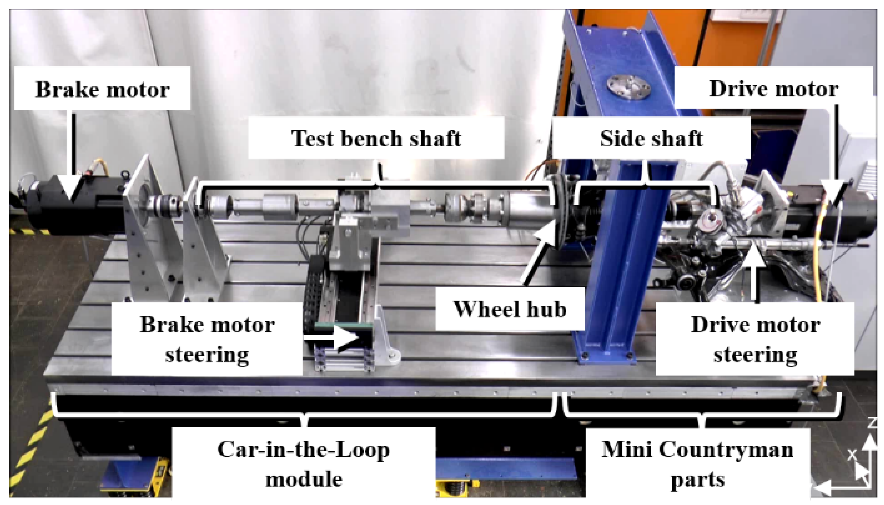
A prototype for the CiL concept that was built in the IMS lab is depicted in Figure 3. For simplification of notation, we refer to the prototype in the following discussions as CiL. More details about the test bench and its modeling are given in [5]. In this work, we focused on the control of the CiL longitudinal dynamics. The control task was to track a reference trajectory of the wheel hub speed using the brake motor torque, while the torque from the drive motor was regarded as a disturbance from the perspective of the test bench control.
In [5], the CiL longitudinal dynamics were modeled as a three-mass-spring-damper system with nonlinear frictions and backlashes. In this contribution, to simplify the case study, we neglected the non-linearity in the system and considered the CiL longitudinal dynamics as an LTI system, which is described in state-space form as (2) with
A = 0 0 1 1 0 0 0 0 1 1 322 , 277 0 23.24 23.12 0 27 , 038.8 48 , 516.0 1.94 9.24 7.27 0 401 , 767.1 0 60.24 60.32 , B = 0 0 0 0 40.16 T , C = 0 0 0 1 0 T .
The output matrix C shows that only the wheel hub speed among all five states was measured.

4.2. Augmented LQT Control with Perfect Model

Since the LQT control framework with the augmented system has the advantage of zero steady-state error, we adopted this method for the study on CiL. A simplified control scheme is illustrated in Figure 4. With y = C x and y r being known, the control system could be augmented with the integrated tracking error of wheel hub speed as an additional state using (3). Furthermore, we also included this state in the exogenous system and simply assumed that it should be constantly zero.
For the case with an LQT with a step command of the wheel hub speed, we could construct the exogenous system for the augmented system as follows:
A a ¯ = 0 0 1 0 , C a ¯ = 1 0 0 0 , E d = 0 0 0 0 0 1 0 0 0 0 0 0 T .
For the augmented system, we constructed the weighting matrix of the cost function with Q a =  diag ( [ Q 1 , Q 2 ] ) and R, with Q 1 being the weighting factor for the tracking error, Q 2 for the augmented state, and R for the system input.
Assume that the real system is completely known, the controllability and observability of the system can easily be examined. Therefore, we can use ( A , B , C ) as the perfect model of the real system to solve the LQT problem as described in Section 3.1.3, by calculating (12) using (13) and (14), with P and Π ϕ obtained by solving (15) and (16). Due to the characteristics of the system state matrix, it was rescaled for more stable matrix operations. For this specific system, it proved to be extremely difficult to find a stable control solution using the perfect model of the real system for the control. A Monte-Carlo simulation with 10 4 repeats with Q 1 , Q 2 and R randomly selected in the range of [ 10 20 , 10 4 ] was performed. As depicted on the left side of Figure 5, only 5 out of the 1 e 4 random combinations of weighting factors contributed to a stable controller.
From an optimization point of view, the model offered many more degrees of freedom for the problem solving than that of the weighting matrices in the cost function. Abandoning a direct physical interpretation of the model for the controller, in the following chapters, we show that a model learned via BO can facilitate a much larger set of stable controllers. It also exhibited an improved control performance. To the best of the authors’ knowledge, this discovery is the first in the LQT-related literature.

4.3. Augmented LQT Control with Model Learned via Bayesian Optimization

Recall that, in Section 4.2, we could not find stable controllers by implementing LQT with augmented states on CiL with perfect knowledge of the ‘real’ system. In other words, we used a perfect model of the ‘real’ system for the controller in the simulation study. Now, we revisit the augmented LQT control problem and implement the algorithm of model learning via BO as described in Algorithm 1 on the simulated CiL. For this learning task, we assume a priori that the system is a three mass-spring-damper LTI system, for which the physical parameters (mass, spring stiffness etc.) are unknown. In particular, we use BO to learn the the unknown entries in the system state matrix A B O and input matrix B B O for the LQT controller directly in closed-loop conditions. These unknown entries are dependent on the physical parameters of the CiL. More specifically, we have Θ = [ θ 1 , θ 2 , , θ 12 ] integrated in
A B O = 0 0 1 1 0 0 0 0 1 1 θ 1 0 θ 2 θ 3 0 θ 4 θ 5 θ 6 θ 7 θ 8 0 θ 9 0 θ 10 θ 11 , B B O = 0 0 0 0 θ 12 T .
This implementation of BO was based on the toolbox “bayesopt” in MATLAB/Simulink 2022a. For this optimization task, we chose EI as the acquisition function. The exploration ratio was set to 0.5 . GP was selected as the surrogate model, with Matern 2/5 [17] as the kernel. Since no prior knowledge about the mapping of the cost function to model parameters was given, we assumed zero mean for all random variables in the GP prior. In the learning stage, the reference trajectory of the wheel hub speed with a step command of 10 rad / s at 1 s was used. The duration of the simulation was set to 20 seconds. The optimization objective function as described in (17) for the augmented LQT problem was implemented for BO, after averaging over time and logarithmization. With trivial weightings of Q 1 = 1 , Q 2 = 8 , R = 1 and 30 random initialization, we obtained an optimized BO model ( A B O , B B O ) for the LQT controller in N = 500 iterations:
A B O = 0 0 1 1 0 0 0 0 1 1 565 , 390 0 490.92 106.63 0 824 , 120 563 , 610 323.5 475.87 278.53 0 271 , 700 0 314.96 83.672 , B B O = 0 0 0 0 95.36 T .
This model is called BO model in the following sections for simplification of notation. A Monte-Carlo simulation with the same settings as described in Section 4 was performed and the simulation results are illustrated on the right side of Figure 5. In total, 1782 stable controllers were obtained, which was a significant improvement compared to the sparse stable controller set with the perfect model of the ‘real’ system. In Figure 6, a comparison of the step command response is depicted. The best result with the perfect model (lower left point in the left plot of Figure 5) is shown in red color. A representative point with comparable overall cost from the results with the BO model is presented in blue. As illustrated, the controller with BO model injected more energy into the system, to allow a much faster transient dynamic.
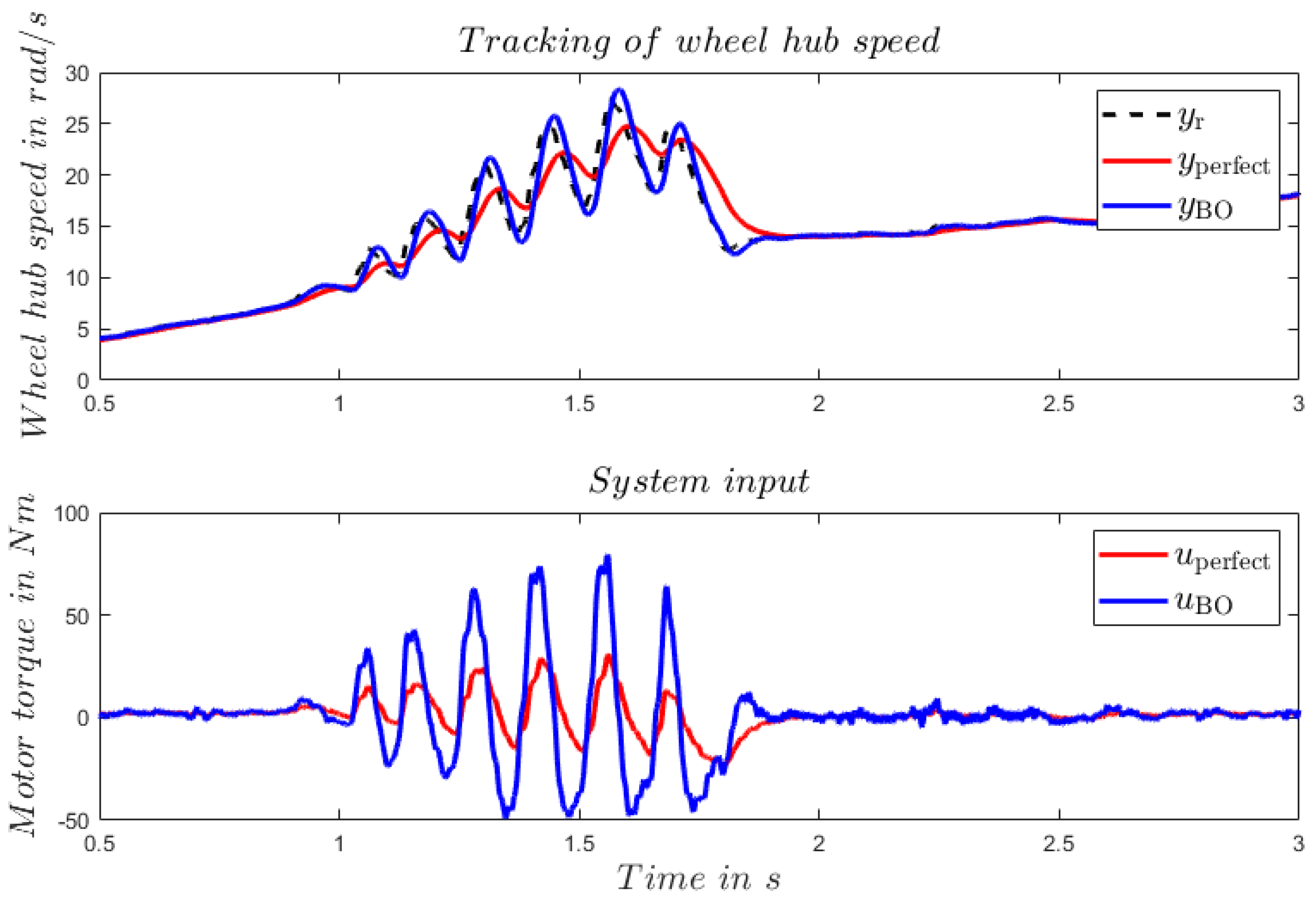
In practice, it is difficult to describe an arbitrary reference trajectory of wheel hub speed, i.e., the vehicle velocity with the formulation of (10). It is trivial to consider the reference trajectory as small step commands at each sample time, and therefore one can use the same controller for an arbitrary reference trajectory as for the step command. The practicability of this simplification was validated using a recorded wheel hub speed from real-world driving as a reference trajectory, where the tire slip phenomenon was captured. The results are illustrated in Figure 7. Due to the much faster transient dynamic, the controller with BO model tracked the reference trajectory much better than its counterpart with the perfect model.

4.4. Discussion on the Model Learned via Bayesian Optimization

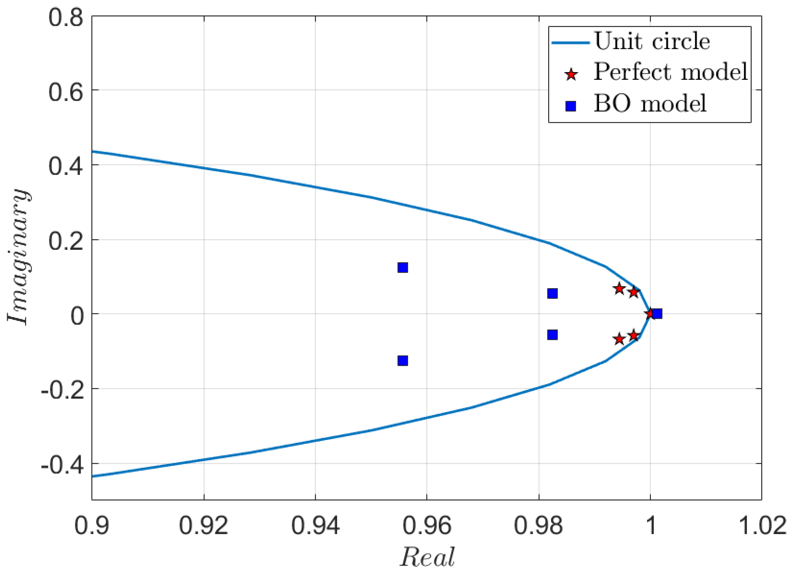
In this section, we demonstrate that within the LQT control framework, a controller with a learned model can provide a significantly more stable solution for certain systems (e.g., CiL) than a controller with perfect knowledge of the system. However, inherently, a model–plant mismatch is highly possible for the former case. Indeed, a comparison of the eigenvalues of the system (27) and (30) after discretization revealed that the learned model did not reflect the dynamics of the ‘real’ system, as shown in Figure 8. The model learned via BO was open-loop unstable with an eigenvalue outside the unit circle, while the ‘real’ system was marginally more stable.
The fact of plant–model mismatch raises two concerns. The first concern is over-fitting. However, it is shown that with carefully designed experiments, one can learn a performance-driven model for control that excites the dynamic spectrum of interest for the control task at hand. This is a very useful insight. In fact, the authors encourage readers to use the system itself to (semi-)automatically generate the information of interest [31]. A second concern is the stability margin. In the case of a linear quadratic Gaussian (LQG) controller, as famously stated in [38], there is none for this class. This implies that the stability margin is inherently system-specific. In practical applications, we carefully examine the robustness of the controller individually. For CiL, the test scenarios can be categorized into several dynamic ranges and represented with certain test signals. In this case, the robustness is examined directly in an experimental setup. Examples of the systematic study of robustness and integration into the algorithm for performance-driven control can be found in [23,29,39]. This is outside the scope of this paper. The intention of the authors was to showcase the possibilities opened up by this new approach, with the focus on the industrial practicability.

4.5. Effectiveness of Bayesian Optimization

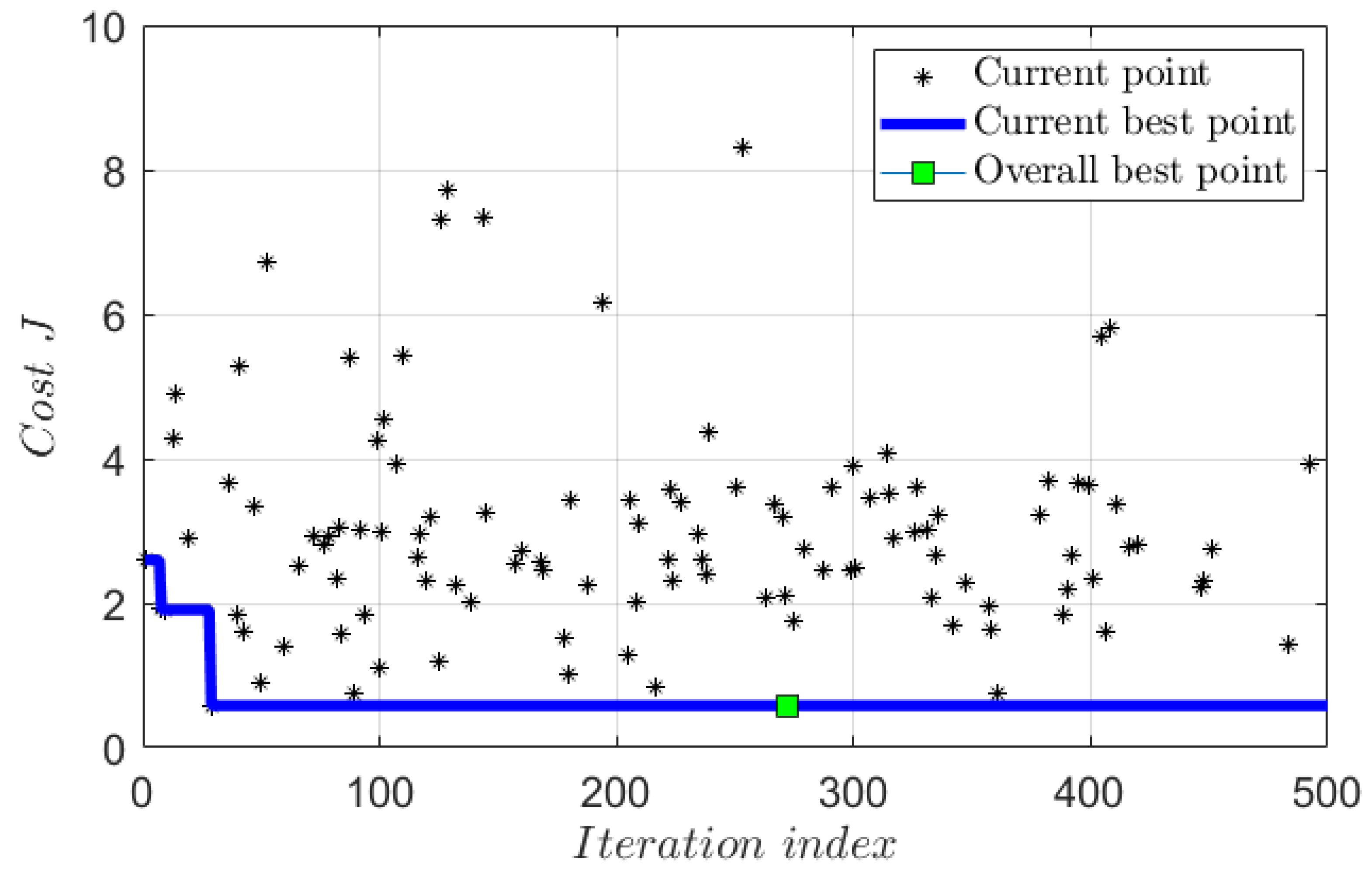
The BO algorithm for model learning converged fast in the case of CiL. In Figure 9, a representative closed-loop system performance of CiL in the simulation over the iteration steps during the model learning is illustrated. The blue line visualizes the best performance up to most recent iteration. With sufficient initial seeds of parameter sets randomly selected from the parameter space, the BO algorithm converged in a very effective manner. Therefore, in the case of CiL, the performance-driven approach together with BO was data-efficient and suitable for experimental controller design.

5. Conclusions

In this contribution, we discussed a control method for LQT with zero steady-state error. This was realized by augmenting the system states with an integrated tracking error. The general LQT control framework introduced in [7] can be used for the augmented system, which has not previously been mentioned in the literature.
A possible reason for this could be that, due to the augmentation of the system, as well as the introduction of the exogenous system, the dimension of the Sylvester Equation (16) could be increased quite significantly when many states or outputs are to be tracked in the system. This fact could be a limitation of the method.
On the other hand, an interesting discovery for the specific system of CiL is that almost no stable solutions can be found with a perfect model of the ‘real’ system for LQT control. However, a stable and better performing solution can be found more easily with a controller model learned via BO. Based on the learned model, the controller parameter can be further tuned in a sequential step and achieve the desired performance with respect to certain objectives.
Currently, the conclusions drawn in this contribution were based on numerical simulations. All system states were assumed to be known. In addition, nonlinear effects of the real system were not considered. In future works, a control method for nonlinear systems in combination with a state estimator should be studied further, to pave the way for practical applications. It would also be interesting to prove the feasibility and stability of the method mathematically in more general terms. For example, how might the model learned via BO provide an alternative approach to the augmented LQT controller design for the specific class of systems that are similar to CiL, which is notoriously difficult to solve with a perfect model of the ‘real’ system as the controller model. Moreover, due to the state augmentation, as well as the introduction of the exogenous system, the dimensions involved in the controller design can increase significantly for systems with high dimensions and/or multiple tracking states. Further investigation is required to fully understand the efficacy of BO for modeling systems with higher dimensions.

Author Contributions

Conceptualization, G.G.; methodology, G.G.; software, G.G.; validation, G.G.; writing—original draft preparation, G.G.; writing—review and editing, P.J.; visualization, G.G.; supervision, S.R. All authors have read and agreed to the published version of the manuscript.

Funding

This research received no external funding.

Data Availability Statement

Data are contained within the article.

Conflicts of Interest

The authors declare no conflicts of interest.

References

  1. Ahlert, A. Ein Modellbasiertes Regelungskonzept für Einen Gesamtfahrzeug Dynamikprüfstand; Springer: Berlin/Heidelberg, Germany, 2020. [Google Scholar] [CrossRef]
  2. Gao, Y.; Zhao, X.; Xu, Z.; Cheng, J.; Wang, W. An Indoor Vehicle-in-the-Loop Simulation Platform Testing Method for Autonomous Emergency Braking. J. Adv. Transp. 2021, 2021, 8872889. [Google Scholar] [CrossRef]
  3. Siegl, S.; Ratz, S.; Düser, T.; Hettel, R. Vehicle-in-the-Loop at Testbeds for ADAS/AD Validation. Atzelectronics Worldw. 2021, 16, 62–67. [Google Scholar] [CrossRef]
  4. Schyr, C.; Inoue, H.; Nakaoka, Y. Vehicle-in-the-Loop Testing—A Comparative Study for Efficient Validation of ADAS/AD Functions. In Proceedings of the 2022 IEEE International Conference on Connected Vehicle and Expo (ICCVE), Lakeland, FL, USA, 7–9 March 2022; pp. 1–8. [Google Scholar] [CrossRef]
  5. Fietzek, R. Modellbildung, Regelung und Realisierung eines Neuartigen Konzepts für Einen Gesamtfahrzeugprüfstand; Forschungsberichte Mechatronische Systeme im Maschinenbau, Shaker: Aachen, Germany, 2014. [Google Scholar]
  6. Rinderknecht, S.; Fietzek, R.; Meier, T. Control Strategy for the Longitudinal Degree of Freedom of a Complete Vehicle Test Rig; Technical report; SAE Technical Paper: Detroit, MI, USA, 2012. [Google Scholar]
  7. Bernhard, S. Time-Invariant Control in LQ Optimal Tracking: An Alternative to Output Regulation. IFAC-PapersOnLine 2017, 50, 4912–4919. [Google Scholar] [CrossRef]
  8. Bauer, P.; Bokor, J. Development and performance evaluation of an infinite horizon LQ optimal tracker. Eur. J. Control 2018, 39, 8–20. [Google Scholar] [CrossRef]
  9. Park, J.H.; Han, S.; Kwon, W.H. LQ tracking controls with fixed terminal states and their application to receding horizon controls. Syst. Control Lett. 2008, 57, 772–777. [Google Scholar] [CrossRef]
  10. Willems, J.L.; Mareels, I.M. A rigorous solution of the infinite time interval LQ problem with constant state tracking. Syst. Control Lett. 2004, 52, 289–296. [Google Scholar] [CrossRef]
  11. Modares, H.; Lewis, F.L. Linear Quadratic Tracking Control of Partially-Unknown Continuous-Time Systems Using Reinforcement Learning. IEEE Trans. Autom. Control 2014, 59, 3051–3056. [Google Scholar] [CrossRef]
  12. Hagiwara, T.; Yamasaki, T.; Araki, M. Two-degree-of-freedom design method of LQI servo systems: Disturbance rejection by constant state feedback. Int. J. Control 1996, 63, 703–719. [Google Scholar] [CrossRef]
  13. Barbieri, E.; Alba-Flores, R. On the infinite-horizon LQ tracker. Syst. Control Lett. 2000, 40, 77–82. [Google Scholar] [CrossRef]
  14. Brochu, E.; Cora, V.M.; De Freitas, N. A tutorial on Bayesian optimization of expensive cost functions, with application to active user modeling and hierarchical reinforcement learning. arXiv 2010, arXiv:1012.2599. [Google Scholar]
  15. Khosravi, M.; Koenig, C.; Maier, M.; Smith, R.S.; Lygeros, J.; Rupenyan, A. Safety-Aware Cascade Controller Tuning Using Constrained Bayesian Optimization. IEEE Trans. Ind. Electron. 2023, 70, 2128–2138. [Google Scholar] [CrossRef]
  16. Fröhlich, L.P.; Küttel, C.; Arcari, E.; Hewing, L.; Zeilinger, M.N.; Carron, A. Contextual tuning of model predictive control for autonomous racing. In Proceedings of the 2022 IEEE/RSJ International Conference on Intelligent Robots and Systems (IROS), Kyoto, Japan, 23–27 October 2022; pp. 10555–10562. [Google Scholar]
  17. Frazier, P.I. A tutorial on Bayesian optimization. arXiv 2018, arXiv:1807.02811. [Google Scholar]
  18. Wang, X.; Jin, Y.; Schmitt, S.; Olhofer, M. Recent Advances in Bayesian Optimization. ACM Comput. Surv. 2023, 55, 1–36. [Google Scholar] [CrossRef]
  19. Paulson, J.A.; Tsay, C. Bayesian optimization as a flexible and efficient design framework for sustainable process systems. arXiv 2024, arXiv:2401.16373. [Google Scholar]
  20. Coutinho, J.P.; Santos, L.O.; Reis, M.S. Bayesian Optimization for automatic tuning of digital multi-loop PID controllers. Comput. Chem. Eng. 2023, 173, 108211. [Google Scholar] [CrossRef]
  21. König, C.; Ozols, M.; Makarova, A.; Balta, E.C.; Krause, A.; Rupenyan, A. Safe risk-averse bayesian optimization for controller tuning. IEEE Robot. Autom. Lett. 2023, 8, 8208–8215. [Google Scholar] [CrossRef]
  22. Wabersich, K.P.; Taylor, A.J.; Choi, J.J.; Sreenath, K.; Tomlin, C.J.; Ames, A.D.; Zeilinger, M.N. Data-Driven Safety Filters: Hamilton-Jacobi Reachability, Control Barrier Functions, and Predictive Methods for Uncertain Systems. IEEE Control Syst. 2023, 43, 137–177. [Google Scholar] [CrossRef]
  23. Stenger, D.; Ay, M.; Abel, D. Robust Parametrization of a Model Predictive Controller for a CNC Machining Center Using Bayesian Optimization. IFAC-PapersOnLine 2020, 53, 10388–10394. [Google Scholar] [CrossRef]
  24. Neumann-Brosig, M.; Marco, A.; Schwarzmann, D.; Trimpe, S. Data-Efficient Autotuning with Bayesian Optimization: An Industrial Control Study. IEEE Trans. Control Syst. Technol. 2020, 28, 730–740. [Google Scholar] [CrossRef]
  25. Sorourifar, F.; Makrygirgos, G.; Mesbah, A.; Paulson, J.A. A Data-Driven Automatic Tuning Method for MPC under Uncertainty using Constrained Bayesian Optimization. IFAC-PapersOnLine 2021, 54, 243–250. [Google Scholar] [CrossRef]
  26. Chakrabarty, A.; Benosman, M. Safe learning-based observers for unknown nonlinear systems using Bayesian optimization. Automatica 2021, 133, 109860. [Google Scholar] [CrossRef]
  27. Grande, R.C.; Chowdhary, G.; How, J.P. Experimental validation of Bayesian nonparametric adaptive control using Gaussian processes. J. Aerosp. Inf. Syst. 2014, 11, 565–578. [Google Scholar] [CrossRef]
  28. Doekemeijer, B.M.; van der Hoek, D.C.; van Wingerden, J.-M. Model-based closed-loop wind farm control for power maximization using Bayesian Optimization using Bayesian optimization: A large eddy simulation study. In Proceedings of the 3rd IEEE Conference on Control Technology and Applications, City University of Hong Kong, Hong Kong, China, 19–21 August 2019; IEEE: Piscataway, NJ, USA, 2019. [Google Scholar] [CrossRef]
  29. Berkenkamp, F.; Schoellig, A.P. Safe and robust learning control with Gaussian processes. In Proceedings of the 2015 IEEE European Control Conference (ECC), Linz, Austria, 15–17 July 2015; pp. 2496–2501. [Google Scholar] [CrossRef]
  30. Gevers, M. Identification for Control: From the Early Achievements to the Revival of Experiment Design. Eur. J. Control 2005, 11, 335–352. [Google Scholar] [CrossRef]
  31. Hjalmarsson, H. From experiment design to closed-loop control. Automatica 2005, 41, 393–438. [Google Scholar] [CrossRef]
  32. Bansal, S.; Calandra, R.; Xiao, T.; Levine, S.; Tomlin, C.J. Goal-driven dynamics learning via Bayesian optimization. In Proceedings of the 2017 IEEE 56th Annual Conference on Decision and Control (CDC), Melbourne, Australia, 12–15 December 2017; pp. 5168–5173. [Google Scholar]
  33. Young, P.C.; Willems, J.C. An approach to the linear multivariable servomechanism problem. Int. J. Control 1972, 15, 961–979. [Google Scholar] [CrossRef]
  34. Malkapure, H.G.; Chidambaram, M. Comparison of Two Methods of Incorporating an Integral Action in Linear Quadratic Regulator. IFAC Proc. Vol. 2014, 47, 55–61. [Google Scholar] [CrossRef]
  35. Singh, A.K.; Pal, B.C. An extended linear quadratic regulator for LTI systems with exogenous inputs. Automatica 2017, 76, 10–16. [Google Scholar] [CrossRef]
  36. Mukherjee, S.; Bai, H.; Chakrabortty, A. Model-based and model-free designs for an extended continuous-time LQR with exogenous inputs. Syst. Control Lett. 2021, 154, 104983. [Google Scholar] [CrossRef]
  37. Piga, D.; Forgione, M.; Formentin, S.; Bemporad, A. Performance-Oriented Model Learning for Data-Driven MPC Design. IEEE Control Syst. Lett. 2019, 3, 577–582. [Google Scholar] [CrossRef]
  38. Doyle, J. Guaranteed margins for LQG regulators. IEEE Trans. Autom. Control 1978, 23, 756–757. [Google Scholar] [CrossRef]
  39. Alanwar, A.; Stürz, Y.; Johansson, K.H. Robust data-driven predictive control using reachability analysis. Eur. J. Control 2022, 68, 100666. [Google Scholar] [CrossRef]
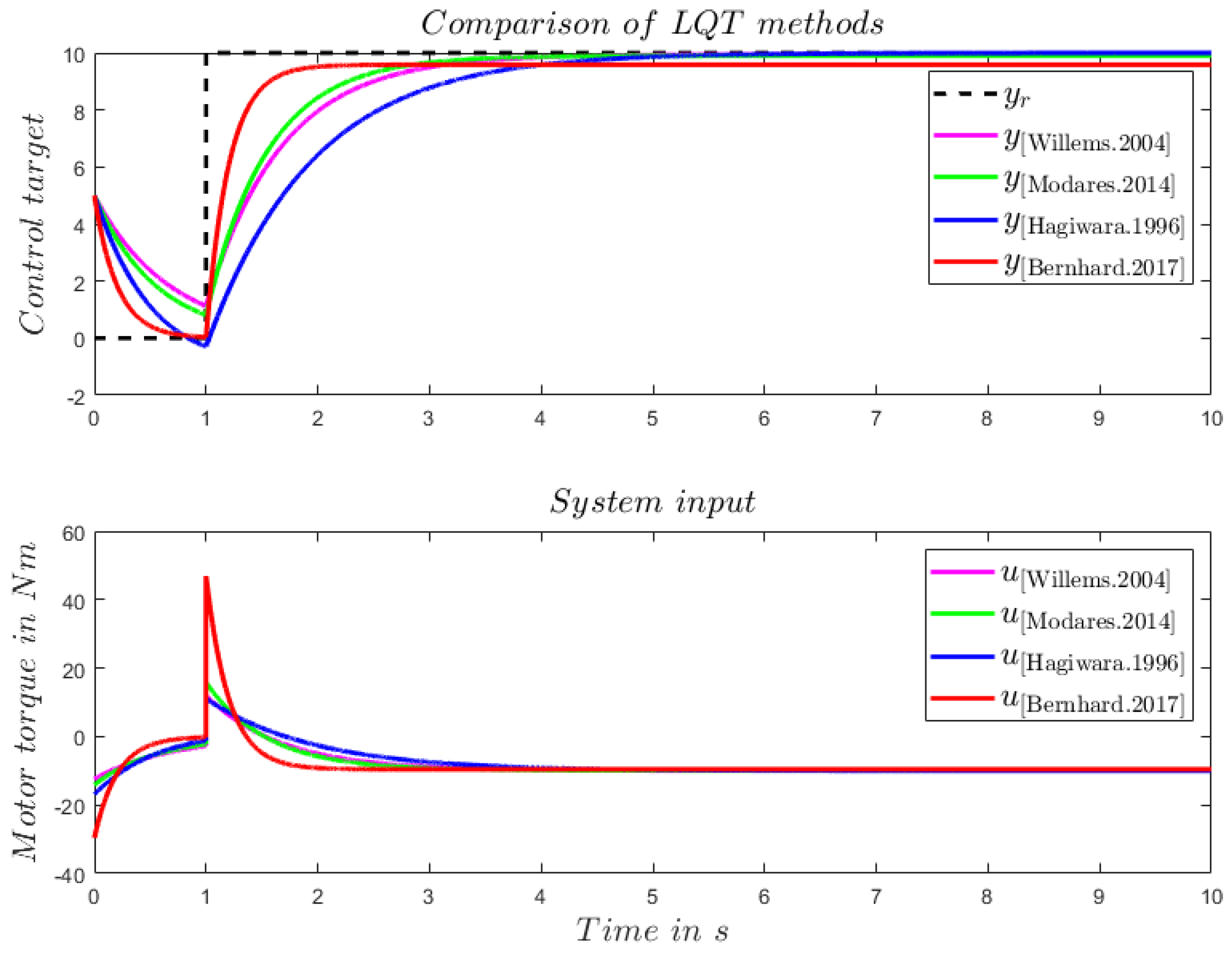
Figure 1. Tracking of a step command by an LTI system with A = 1, B = 1, and C = 1 using the different LQT control methods mentioned above. The same amount of input energy was injected into the system for all control methods: [7,10,11,12].
Vehicles 06 00062 g001
Figure 2. Tracking of a step command using an LTI system with A = 1 , B = 1 , C = 1 . An LQT control framework with the original system model (red line) and augmented system model (blue line) are implemented. The same amount of input energy is injected into the system in both control laws.
Vehicles 06 00062 g002
Figure 3. Car-in-the-Loop test bench prototype.
Vehicles 06 00062 g003
Figure 4. Control scheme for the CiL longitudinal dynamics with augmented LQT controller.
Vehicles 06 00062 g004
Figure 5. Stable controller set with Monte Carlo simulation. Q 1 , Q 2 and R are randomly selected in the range of [ 10 20 , 10 4 ] For ease of reading, the cost evaluation is averaged over the sample numbers and logarithmized. Left: stable controller set with perfect model of the real system, right: stable controller set with learned model via BO.
Vehicles 06 00062 g005
Figure 6. Comparison of the step command response with the augmented LQT controller using a perfect model of the ‘real’ system and the BO model. The overall cost for both controllers was comparable.
Vehicles 06 00062 g006
Figure 7. Comparison of the tracking of real measurement data with the augmented LQT controller using a perfect model of the ‘real’ system and the BO model.
Vehicles 06 00062 g007
Figure 8. Comparison of the eigenvalues of the perfect model and the BO model for the augmented LQT controller.
Vehicles 06 00062 g008
Figure 9. Cost of the augmented LQT controller in performance-driven model learning via BO over the performed iterations.
Vehicles 06 00062 g009
Disclaimer/Publisher’s Note: The statements, opinions and data contained in all publications are solely those of the individual author(s) and contributor(s) and not of MDPI and/or the editor(s). MDPI and/or the editor(s) disclaim responsibility for any injury to people or property resulting from any ideas, methods, instructions or products referred to in the content.