Modeling and Validation of a Passenger Car Tire Using Finite Element Analysis

Abstract

This paper focuses on the modeling and analysis of a four-groove passenger car tire, size 235/55R19, using finite element analysis. The Mooney–Rivlin material model is employed to define the hyperelastic behavior of the tire rubber compounds for all solid elements. The tire rim is modeled as a rigid body using aluminum alloy material, and the beads are modeled as beam elements using steel material. The tire model is validated in both static and dynamic domains through several simulations and is compared to published measured data. The tire is validated using footprint and vertical stiffness tests in the static domain. In the static footprint test, a steady-state vertical load is applied, and the tire–road contact area is computed. In the vertical stiffness test, a ramp vertical load is applied, and the tire’s vertical displacement is measured to calculate the tire’s vertical stiffness. In the dynamic domain, the tire is validated using drum-cleat and cornering tests. In the drum-cleat test, a drum with a 2.5 m diameter and a cleat with a 15 mm radius is used to excite the tire structure and obtain the frequency of the vertical and longitudinal first modes of vibration, that is, by applying the fast Fourier transformation (FFT) of the vertical and longitudinal reaction forces at the tire center. In addition to this test, the tire model is pre-steered on a flat surface with a two-degree slip angle and subjected to a steady state linear speed of 10 km/h to predict the cornering force and compute the cornering stiffness. In addition, the effect of tire longitudinal speed on the rolling resistance coefficient is then predicted at zero slip angle using the ISO 28580 rolling resistance test. The findings of this research work provide insights into passenger car tire–road interaction analysis and will be further used to perform tire rubber compound material model sensitivity analysis.

1. Introduction

Tires are the main components in vehicles as they have a significant effect on the vehicle’s performance such as ride, traction, braking, and handling. Moreover, tires’ rolling resistance directly affects the fuel consumption of the vehicle. Therefore, there is an essential need to examine and predict tire performance under various operating conditions. In recent years, several researchers predicted tire behavior with different tools including numerical analysis and empirical analytical simulations in addition to the experimental tests. Experimental tests such as drum-cleat tests or coast-down tests are very time-consuming and costly. As a result, many researchers put a significant effort into modeling prediction of the tire performance with numerical approaches that are an effective source of information for the tire manufacturers and the automotive sectors. The finite element method is one of the most useful and powerful tools that is being used for designing and analyzing tires. The first application of the finite element method in tire industries returned to 1970 decay by the introduction of tire science technology journals.

The first effort to model two-dimensional tires referred to the 1970 decay and the first footprint modeling refers to 1980. In 1973, Zorowski et al. [1] was one of the pioneers who presented the idea of the use of finite element methods to study the dynamic behavior of tires. He proposed applying finite element techniques for tire modeling and mathematical prediction. Moreover, he used a classical membrane theory for designing tire plies. The results of his study can be used in the future for tire design and applying constraints on carcass shape. In 1974, Ridha et al. [2] presented a linear finite element model for the deformation of tires due to shrinkage. This analysis was performed using composite theory for modeling the material properties and structural behavior. The analysis is performed to fit the mold shape into the final shape of the tire. The shrink forces were extracted, and the results showed a good correlation between calculated and experimental displacement.

In 1978, Kennedy et al. [3] performed a simulation on the analysis of the radial automobile tire. The tire was undergoing steady-state rotation using a finite element method. A quasi-static method was implemented to solve the static analysis of the rotating tire. One of the advantages of this method was shortening the solution time for the tire simulation. The tire was modeled two-dimensionally with an elastic structure, and then a full three-dimensional tire was generated. The tire model was subjected to ground contact, and a point load excitation was applied to the tire. The result showed a good agreement with the experimental variables including damping and the effect of inertia components. It should be noted that to modify the damping, a two-element Kelvin–Voight viscoelastic material model was adopted for the simulation.

In 2000, Shiraishi et al. [4] presented an explicit finite element method to model the dynamically rolling tire. The internal construction of the tire and the complicated pattern shape of the tire were modeled with full details and geometry. One major drawback of this work was the higher simulation time in contrast to the other techniques, although it was acceptable for practical tire development. The output results were stated under various rolling conditions, and they were verified with experimental data that revealed enough correlation. As a result, the finite element techniques using explicit methods were considered a useful procedure to model the dynamically rolling tires. In 2000, Kabe et al. [5] presented implicit and explicit simulations using finite element techniques to model a passenger car tire. The cornering simulation was also performed to extract the lateral force of the tire under the state stage. The results were validated using the experimental data from an MTS Flat-Test Tire Test. The predicted cornering results in two different methods including implicit FEA and explicit FEA were compared to the experimental ones and they showed a good correlation between the simulation and the real cornering data from the MTS Flat-Test Tire Test.

In 2006, Ghoreishy et al. [6] presented a finite element model of the steady-state rolling tire using the commercial computer software Abaqus Version 6.4, 2003. An axisymmetric model was imported as a tire section and then generated a three-dimensional tire. Finally, the distribution pressure and shear stress field steady state rolling were compared to the experimental measurement and showed a good correlation with each other. In the same year, Chae [7] performed a frequency analysis and static validation for a real truck tire, 295/75R22.5. The sidewall damping was computed for various tire operating conditions including various load and inflation pressure.

In 2009, Krmela, J. [8] presented a computational method for passenger car radial tire modeling. The tire model was generated using finite element techniques via ANSYS software. The strain-stress analyses were carried on for the proposed FE tire model. All the tire layers have been modeled according to the tire complexity. Tire composite structures including textile cords, steel cords, and elastomer parts of tire carcass were simulated.

In 2016, Lardner et al. [9] analyzed a 445/50R22.5 truck tire in Pam-Crash software. The research aimed to determine the effect of various operating conditions including different tire speeds, inflation pressure, and load on the first frequency mode. The simulation was carried out using a drum-cleat test. The results were validated using the Pam-Crash fast Fourier transform (FFT) algorithm to perform a frequency analysis. FFT is a transformation of forces in the time domain with the help of an optimized discrete Fourier transform (DFT) by decreasing the several orders and reducing the complexion [10,11]. Therefore, a frequency analysis converts the amplitude of tire reaction forces from the time domain to the frequency domain.

In 2017, Krmela [12] presented computational modeling for car tires according to the material identifications. Moreover, experimental testing including dynamic tests of tires and low cyclic loading tests of composites were performed in this work. In addition, tire casings and material parameters identification were included. Furthermore, several analyses including, modal analysis, pressure footprint analyses, and the static test for the prediction of tire radial stiffness were carried out. The tire computational models were generated by implementing hyperelastic and orthotropic material models instead of composite elements of a tire casing. The material characteristics were obtained from the experimental tests.

In 2018, Rafei et al. [13] presented an advanced finite element model for a rolling tire at different tire–road friction conditions to model rolling tires under cornering simulation. The friction was modeled using a thermos-mechanical procedure by developing two Abaqus subroutines. The simulation results were validated using output data from a flat-track machine test. The FEM results revealed that the complexity of the material models and friction have a negligible effect on the lateral force in contrast to aligning moment and pressure distribution on the footprint. In 2018, El-Sayegh et al. [14] performed a cornering analysis of a wide base truck tire 445/50R22.5 over dry and wet surfaces in a virtual software package Pam-Crash. The cornering stiffness and lateral force in addition to the rolling resistance coefficient were computed for this tire.

In 2020, Krmela, J. [15] published a book on the computational and experimental modeling of tires. Moreover, the theory for tire modeling was explained. In this textbook, various tests on tires including static and dynamic testing machines have been described completely. In the same year, El-Sayegh et al. [16] modeled a truck tire size 315/80R22.5 traveling on the gravel soil using finite element analysis. Soli texture was modeled using the Smooth-Particles Hydrodynamics (SPH) method in the Pam-Crash software. In this research, tire–road characteristics were captured using four tire set-ups including (a) a free-rolling steering tire, (b and c) driven tires, and (d) a free-rolling push tire. Tire mechanics’ properties were validated using the experimental tests in Göteborg, Sweden. In 2020, Ali, S.N. SN Ali [17] studied the rolling resistance prediction of the passenger car radial tire using finite element procedures. For this purpose, firstly the deformation of the tire under certain vertical loading was calculated. Moreover, the total required force for deformation was assumed as energy loss in the tire’s rolling resistance. In addition, the finite element simulation results revealed that the lowest rolling resistance is caused by the largest crown angle.

In 2021, Gao et al. [18] performed a study on the tire deformation characteristic under high-speed rolling conditions. The study utilized a three-component tire assembly to model the belt, sidewall, and rim. It was found that the influence of vertical load has a more substantial effect than the tire pressure on rolling deformation. In the same year, Phromjan et al. [19] developed a solid tire model for finite element analysis of compressive loading. The study examined three layers of natural rubber compounds using stress-strain analysis, and an Ogden model was fitted. It was concluded that the footprint characteristics increase with the compression load; however, the contact pressure was not affected.

In 2022, Király [20] modeled the tire-pavement interaction for a radial truck tire using finite element techniques via ABAQUS software. For this purpose, a complex rubber tire model consisting of a large number of elements was generated, and then the tire model was meshed. The contact stress analysis was performed for the FE tire model. The results revealed a good capability for the prediction of the diagonal tire behavior according to the contact areas and stresses.

Recently, in 2023, Lu D et al. [21] presented a detailed tire finite element modeling in addition to the material identification. The viscoelastic properties of tire compounds were taken into account by performing experimental testing via a cyclic tensile test. In addition, the effect of various material modeling on the tire dynamic behavior was observed. The finite element results showed a good agreement compared with the experimental results for the longitudinal force, lateral force, and correction moment. In the same year, Fathi et al. [22] performed a finite element analysis of a Regional Haul Steer II (RHS), 315/80 R22.5 truck tire. The tire interacted on a dry, hard terrain. The cornering characteristics of the tire, including cornering stiffness and lateral force, in addition to the self-aligning moment, were computed under various operating conditions.

This research provides insights into the static and dynamic behavior of tire models at different operating conditions. This paper uses finite element analysis to model and analyze a passenger all-season car tire with four grooves, size 235/55R19. This particular tire size is widely used for both passenger cars and light trucks and is popular in North America. For all solid elements, the hyperelastic behavior of tire rubber compounds is defined using the Mooney–Rivlin material model. Steel is used to model the beads as beam elements and aluminum alloy is used to model the tire rim as a rigid body. Several simulations are used to validate the tire model in both the static and dynamic domains and the results are compared to published measured data. The research work presented in this paper contributes to a better understanding of tire characteristics and the utilization of hyperelastic material to model rubber compounds, especially at high speeds where most of the current models are lacking.

2. Finite Element Tire Modeling

In this research, a four-groove passenger car radial (PCR) tire size 235/55R19 from the Continental Cross Contact LX Sport model is simulated using finite element analysis (FEA). The full finite element tire model is generated using a commercial finite element software named Pam-Crash. Numerical calibration for the tire geometry and size including rim diameter, tire width, tire height, aspect ratio, and weight of the tire and rim are carried out according to the continental tire manufactured data catalog [23], as shown in

Table 1. Comparison between the size and weight of a 235/55R19 101H passenger car tire model and measurements.

Tire Information	Manufacturer * Diameter (mm)	Simulation Diameter (mm)	Manufacturer * Weight (kg)	Simulation Weight (kg)
Rim and Wheel	482.6 (19 inch)	445.27	11.4 (25.13 lbs.)	11.05
Tire	741.68 (29.2 inch)	739.69	13.65 (30.1 lbs.)	14.81

* Manufacturer data are directly taken from the Continental website [23].

. It should be noted that the simulated diameter and weight are reported after the tire is inflated and before it is loaded. During the initial design of the CAD model, these dimensions may vary slightly as the effect of pressure should be taken into consideration.

According to the information stated in the tire catalog, the maximum load for Continental Cross Contact LX Sport 235/55R19 is 8 kN (1819 lbs.) with a maximum inflation pressure of 252 kPa (51 psi). The nominal values for load and inflation pressure are selected as 5 kN and 228 kPa based on the common vehicle’s gross weight and the tire manufacturer’s recommendation, respectively.

Furthermore, in addition to the geometric properties of the tire, tire mechanics and dynamic characteristics such as vertical stiffness, cornering stiffness, and rolling resistance coefficient, in addition to critical vertical frequency, are simulated using finite element analysis. The nominal inflation pressure of 228 kPa and a nominal vertical load of 5 kN are applied to the center of the tire-wheel assembly to calibrate the tire with tire characteristics according to the tire manufacturer data catalog [23]. Moreover, optimizing the diameter of the beads was performed to achieve a reasonable tire weight, which is 14.81 kg. It should be noted that the gravity was defined for the center of the tire by using a curve function with the value of 9.81 m/s² in the Pam-Crash acceleration.

2.1. Meshing Techniques

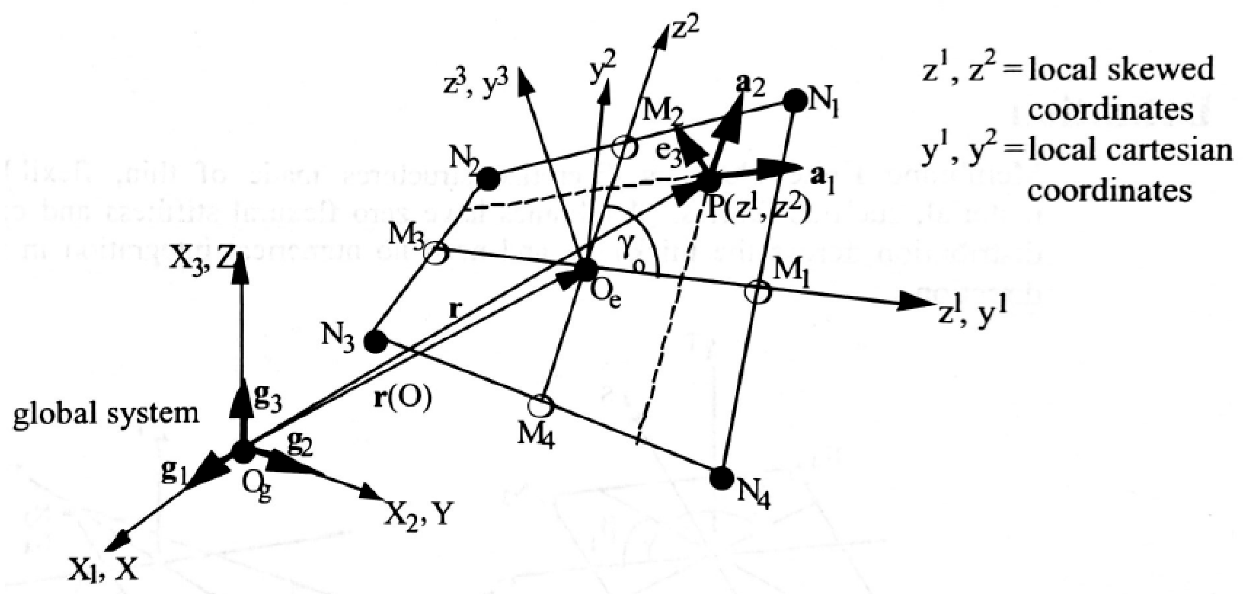
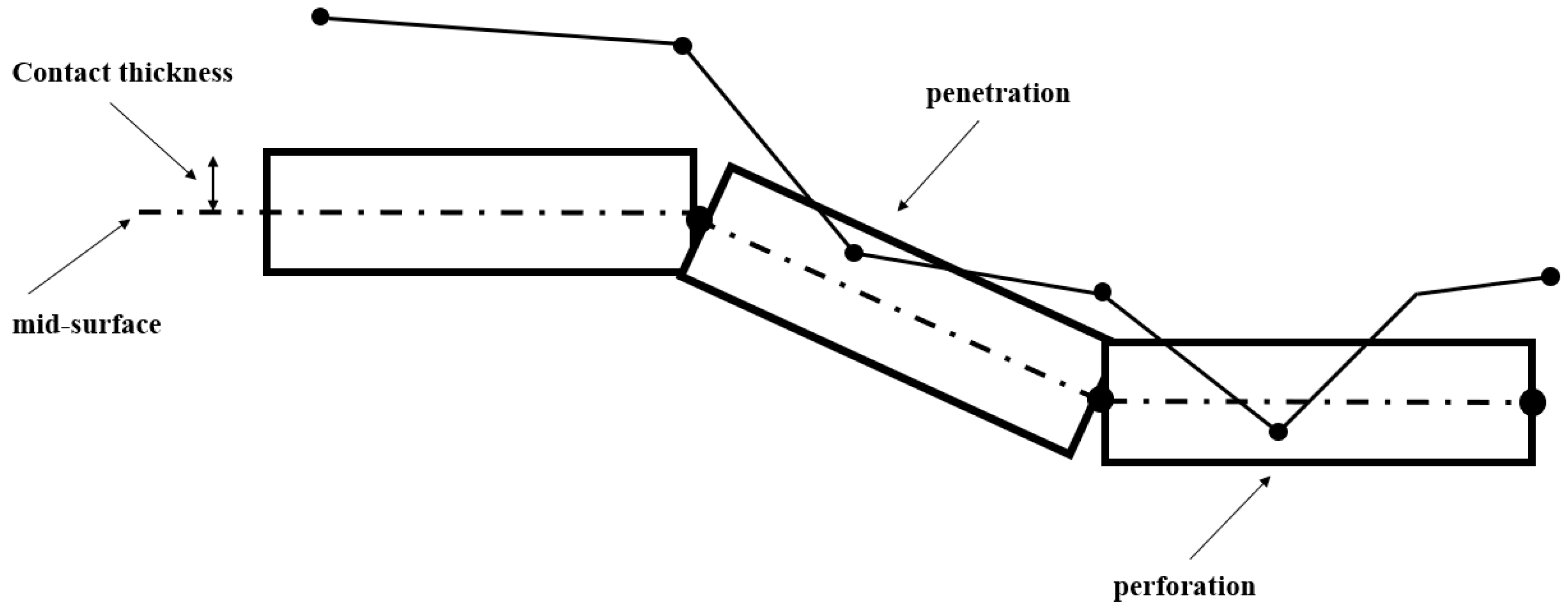
The total tire–road finite element (FE) model in this research consists of 8940 elements and 9617 nodes. All the rubber-like structural components in the tire were meshed using 3D elements including 3240 solid elements (H). The reinforcement cords and rebar layers were modeled using 1D elements including beam elements (BM), 2D elements including thin shell elements (S), and membrane elements (MB). As shown in Figure 1, MB in PAM-SCL is modeled as a two-dimensional element embedded in the three-dimensional space like a 3D solid element (which are tread top and tread base compound and cap ply in this research). They are defined to be formed in a wrapped mid-surface and isoparametric continua [24]. For this purpose, 120 BM were selected to simulate the embedded bead wires in the tire rim area. To model the steel belts, cap plies, and carcass cords, the 3780 S and 1800 MB were chosen.

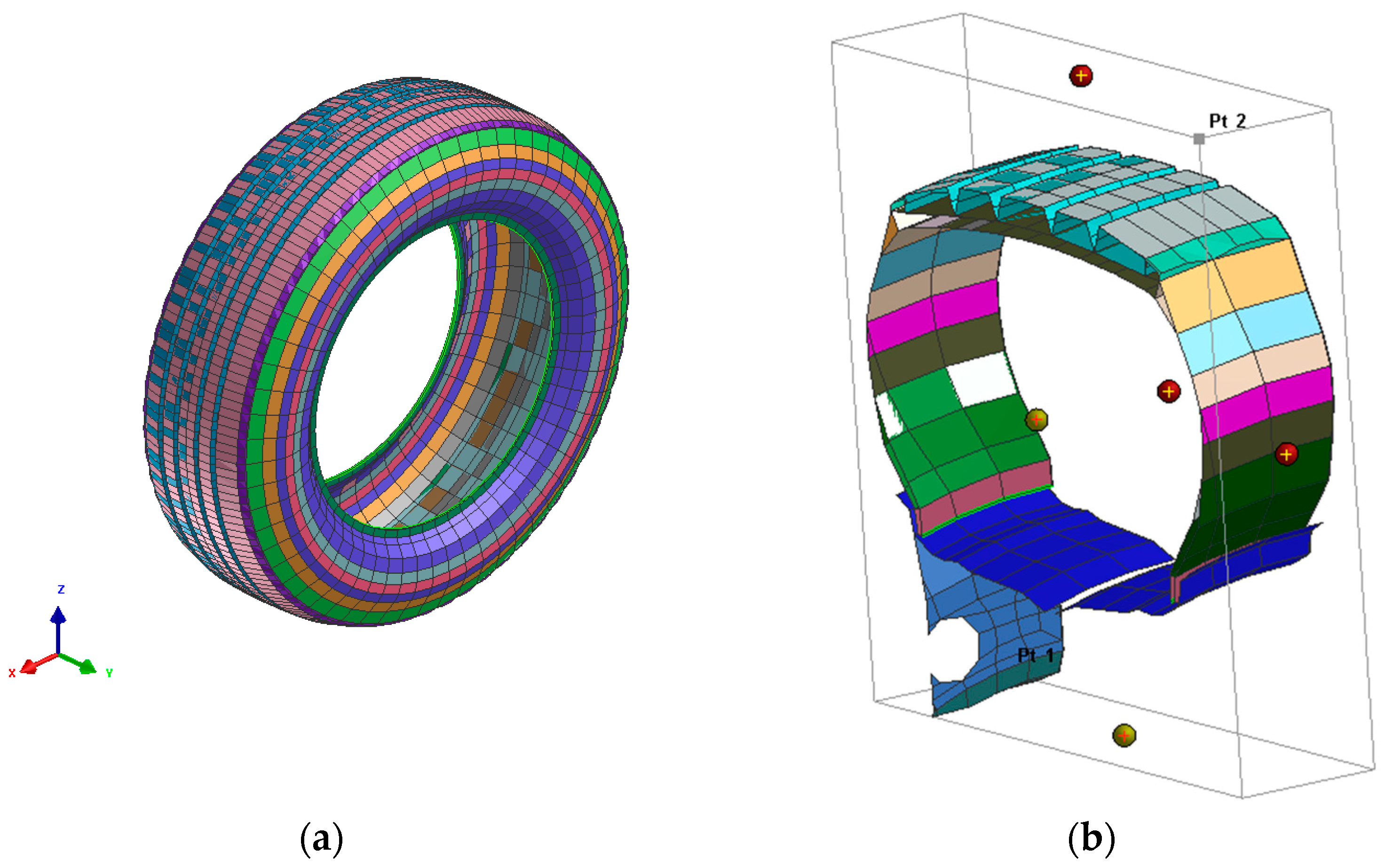
The reason for implementing MB is that these elements have zero flexural stiffness and contact stress distribution across the thickness. Therefore, it is not required to use integration in the thickness direction [25]. Additionally, the road was modeled with the shell elements. Moreover, by assigning solid mesh to the radial-ply tire layers in addition to the reinforcement cords, Figure 2a shows the tire meshed model before post-processing. Figure 2b shows the cross-sectional section of the tire that is rotated 60 equal times in a six-degree increment to obtain the fully rotated tire.

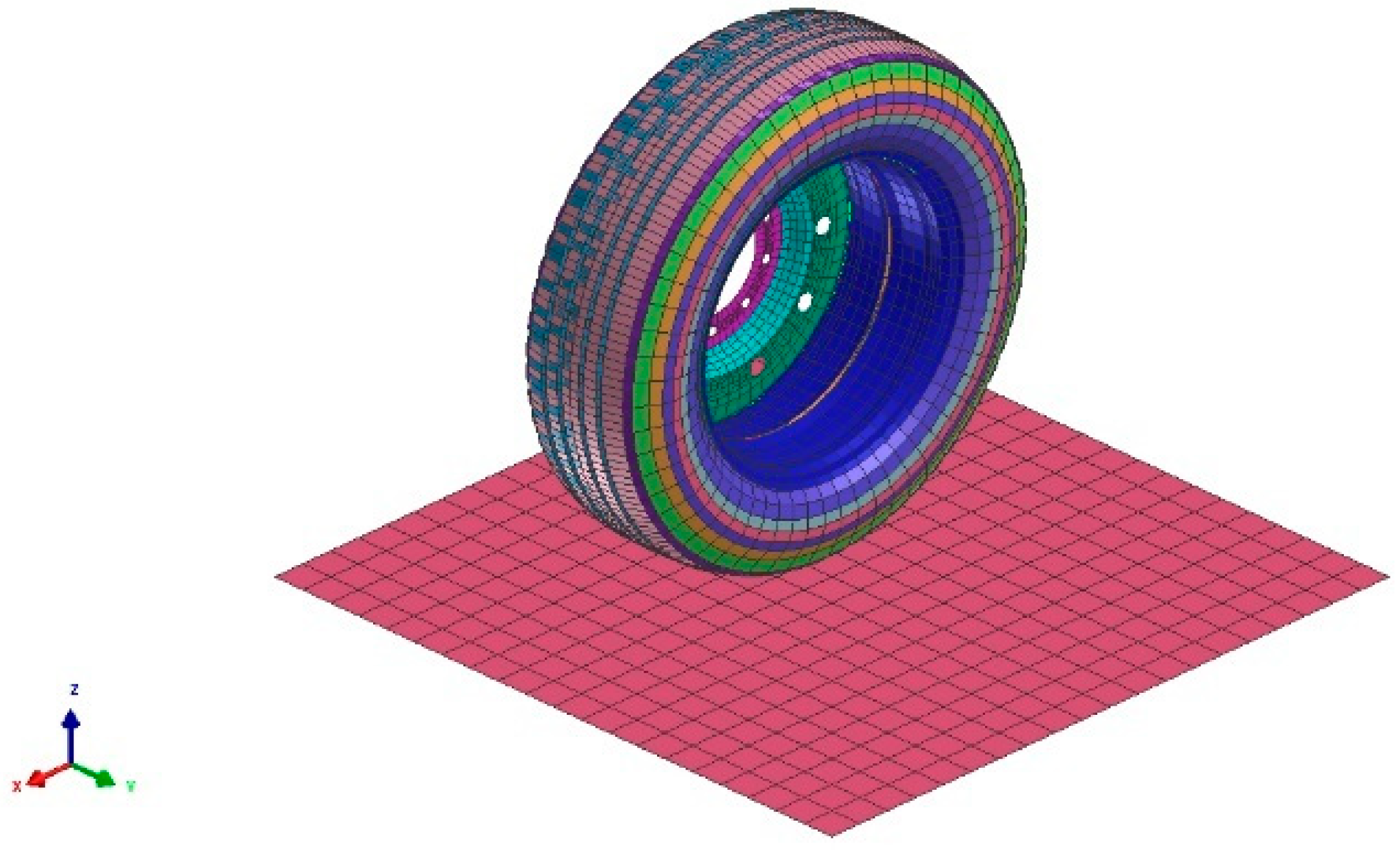
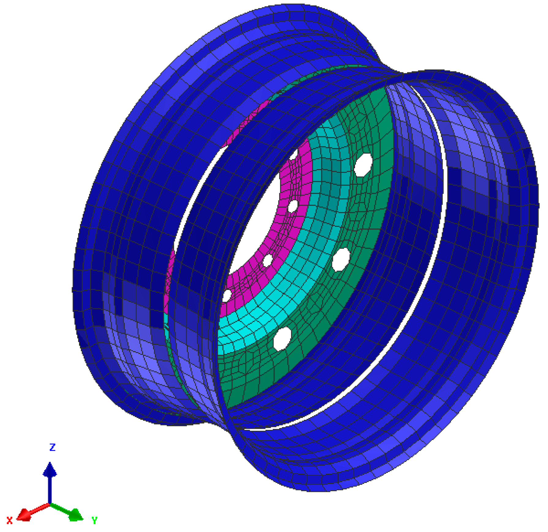
To perform rim mounting, a rigid wheel is selected as shown in Figure 3. To assemble a tire on the wheel, aluminum alloy was assigned to the wheel and the wheel was defined as a rigid body to reduce the complexity of the simulation. This assumption was considered acceptable as the relative stiffness and mass distribution characteristics of the rim in comparison to other layers of the tire are much higher. In addition, in most on-road applications and especially passenger vehicles, the rim is rigid and does not deflect.

2.2. Tire Material Definition

All tire layers including the tread top, tread base, tread shoulders, belt compounds, cap plies, radial plies, sidewall, inner liner, and bead fillers are modeled separately. Moreover, tire reinforcement rebar cords including steel belts, polyester plies, and steel bead wires are modeled with the linear elastic material models. All these modes are assumed to be homogeneous and isotropic. To define the hyperelastic behavior of the tire compounds, the most common material model used widely in tire industry applications is the Mooney–Rivlin material model for medium deformation. The Mooney–Rivlin material model is the expansion of series function models (SEF) by Rivlin [26,27]. Equation (1) is based on first and second strain invariants $I_1, \mathrm{and} I_2$, respectively.

$$W={\displaystyle \sum }_{i=0, j=0}^{\infty }{C}_{ij}{\left(I_1-3\right)}^i{\left(I_2-3\right)}^j$$

(1)

where $C_{ij}$ are the material parameters. The Mooney–Rivlin material model is obtained from Equation (1) when the only parameter materials $C_{10}$ and $C_{01}$ are retained [27].

$$W=C_{10}\left(I_1-3\right)+C_{01}\left(I_2-3\right)$$

(2)

The material parameters for the Mooney–Rivlin hyperelastic model are stated in

Table 2. The Mooney–Rivlin coefficient for tread compounds.

Tire Components	${\mathit{C}}_{10}$ (MPa)	${\mathit{C}}_{01}$ (MPa)	Poisson’s Ratio
Tread Top	2.49	0.67	0.473
Under Tread	0.51	1.86	0.409

. $C_{10}$ and $C_{01}$ are the first (loading) and second (loading) Mooney–Rivlin law coefficients, respectively. Further details regarding the material selection and parameter identification can be found in the previous publication [28].

2.3. Tire–Road Contact Algorithm

In this research, the road is selected as a dry, hard rigid surface. The contact model used is a non-symmetric node-to-segment contact algorithm with an edge treatment [25]. Non-symmetric contact algorithms consider that the contact behavior may vary depending on which side of the interface a node is located. The “edge treatment” suggests that this algorithm considers the specific characteristics or behavior of edges in the simulation. Edge treatment may involve special considerations for how contact is handled along edges, as opposed to the rest of the surface.

To ensure the quality of the solution, a contact thickness of 5 mm and sliding interface penalties of 0.1 were established for the tread elements at the contact patch and road. This is because the slave nodes in the node-to-surface contact should not pierce the master segments. It should be mentioned that there was no symmetry in this treatment. To simulate the actual interactions between tires and roads, a non-penetration node was established to stop tire nodes from entering the elements of the road surface while the analysis was being conducted. To sufficiently cover the distance covered by the tires during the two-second interval, the surface length varied in length.

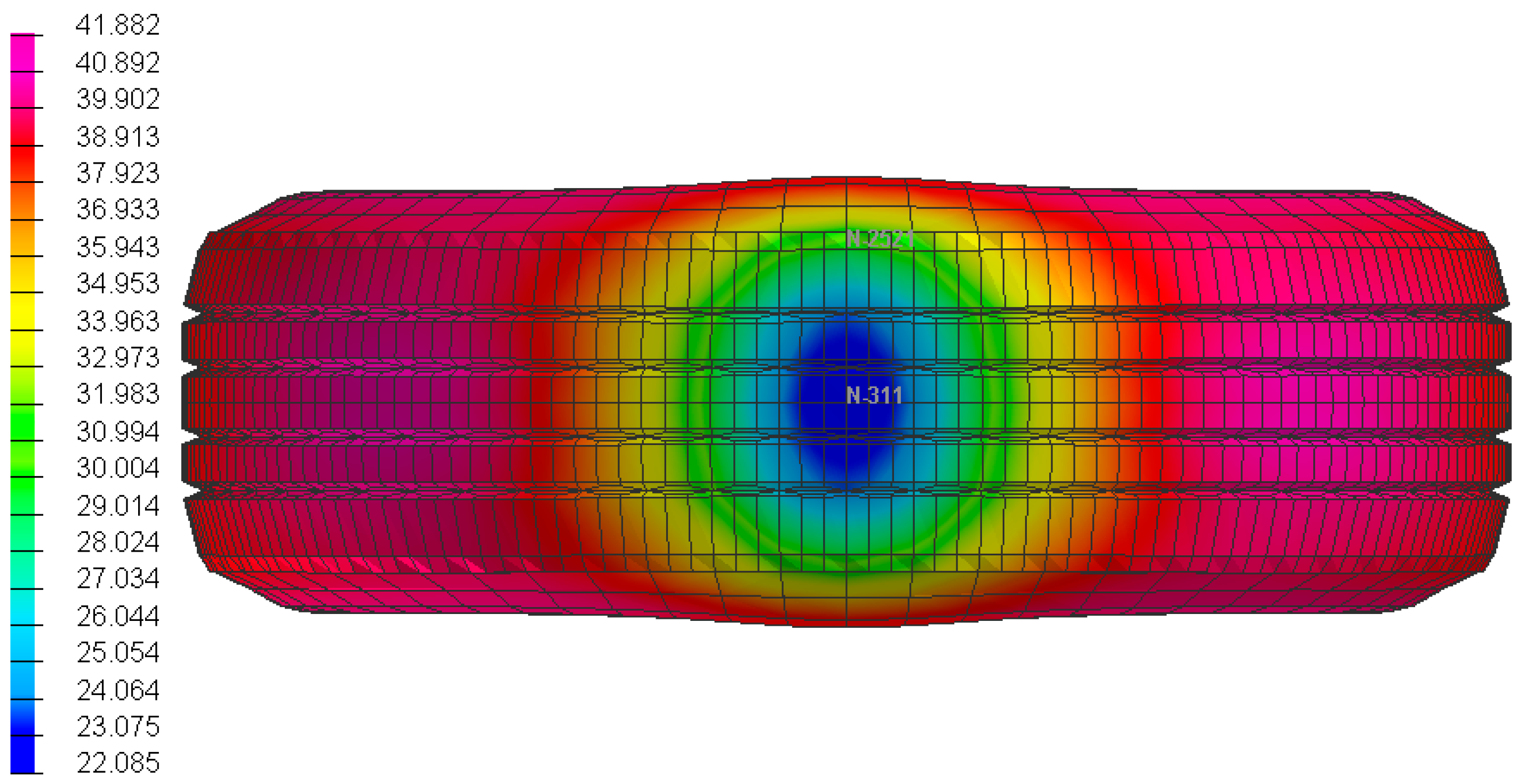
In the whole simulation, the contact node-to-segment was used and the road was meshed with the finer mesh instead of coarse elements to remain in contact between the tire contact patch and road node surface while rolling, as shown in Figure 4.

To determine the tire–road contact interface, the frictional contact with Coulomb’s law was implemented. After a certain point, the bodies of the slave and master no longer adhere to one another. This conditional tangential force, $t_T$, is also known as the sliding force and is explained by the following equation:

$$t_T=-\mu \left|pN\right|\frac{\dot{g_T}}{\dot{g_T}} \mathrm{if} \Vert t_T\Vert >\mu \left|pN\right|$$

where $\mu$ is the sliding friction coefficient representing the frictional properties of the contact interface, $pN$ is the normal contact force or pressure, and $\dot{g_T}$ is the tangential relative velocity between the contacting surfaces. The tire rolls with respect to the road in a sliding condition according to the Arbitrary Lagrangian–Eulerian (ALE) framework.

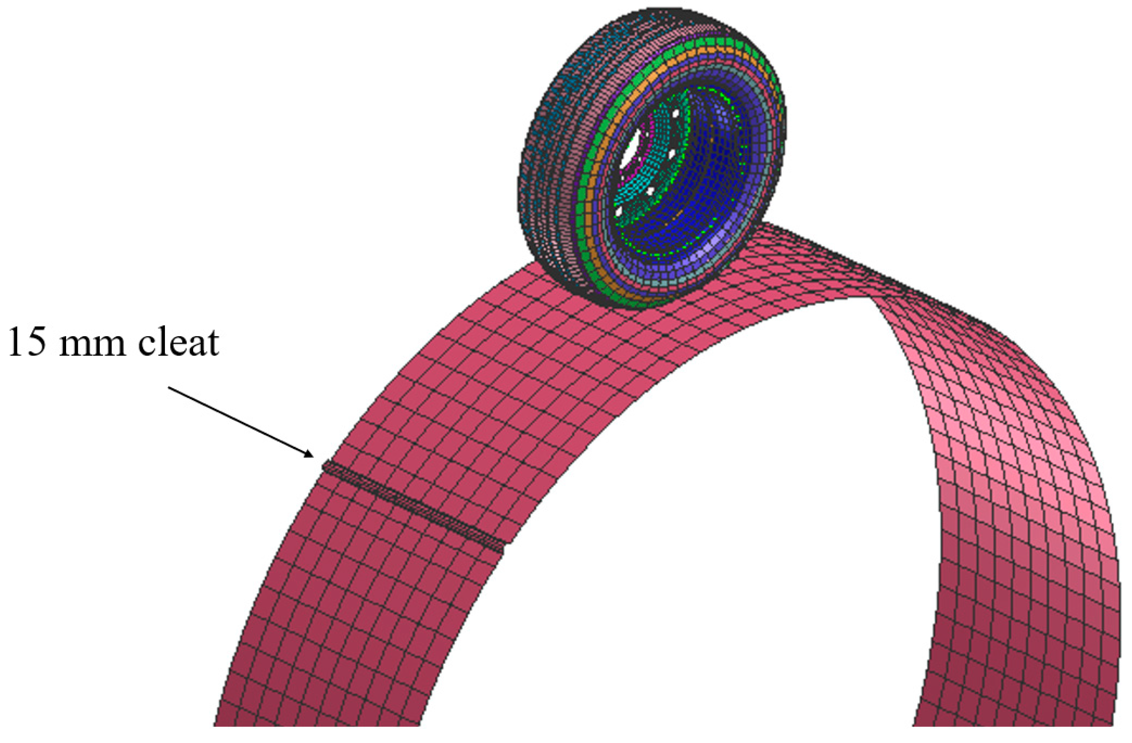
In this case, the tire is selected as a slave and the road is selected as the master according to the algorithm. Figure 5 shows the tire finite element model after appending to the road. To perform the appending tool, a constraint was defined between the tire and the road surface. Considering no penetration from tire contact patch nodes to the road intersections, a 5 mm contact thickness is defined along with implementing Coulomb’s law with a 0.8 friction coefficient for this constraint.

3. FEA Tire Validation

This section presents the tire validation techniques in static and dynamic domains. The static domain includes the footprint, vertical stiffness, longitudinal stiffness, and lateral stiffness. The dynamic domain includes frequency analysis, cornering stiffness, and rolling resistance.

3.1. Static Tire Validation

Based on previous published research [29,30,31], the tire can be validated statically using three different finite element numerical tests. For this purpose, three main different numerical finite element analyses were performed via Pam-Crash software to predict tire static stiffness in all three directions including longitudinal direction, lateral direction, and vertical direction. The total simulation time for each analysis was 2 s. Consequently, 228 kPa inflation pressure and 5 kN vertical load were selected as nominal inflation pressure and nominal load, respectively.

3.1.1. Static Footprint

A static footprint test was performed to validate and to ensure the vertical stiffness test data. To predict the tire contact patch area for the tire–road interaction, a static footprint test was carried out. In contrast to the vertical stiffness test, for static footprint, a steady state vertical load was applied on the center of the tire. Since the vertical displacement of the tire contact patch is along with Z-direction and negative, the normal nodal displacement distribution is contoured and is shown in Figure 6. The central footprint (blue zone) is the least affected area by the applied vertical load on the tire axle since it shows the minimum vertical displacement. According to Figure 6, as this tire features a four-groove design, the surface of the tire in the tread top area, along with the tread pattern, exhibits more curvature shapes during interaction with the road surface. Subsequently, this region undergoes a transition towards straightening, resulting in increased resistance to pressure. Consequently, the elements, in addition to the footprints, generate more displacement under specific static loading in the tire side areas. The purple areas in the figure illustrate the maximum displacement, measuring approximately 41.882 mm. Notably, this maximum nodal displacement is observed at the tire shoulder, particularly in passenger car tires.

3.1.2. Tire Static Vertical Stiffness

To predict tire vertical stiffness, a static vertical stiffness test is carried out with three different inflation pressures including 172 kPa, 228 kPa, and 352 kPa, as well as three different maximum vertical loads including 3.5 kN, 5 kN, and 8 kN. This test is carried out by applying a quasi-static ramp vertical load up to the values listed above on the tire center reference point. For the vertical stiffness, the test tire is not allowed to rotate in any direction and is only allowed to move in the vertical direction. The vertical stiffness of the tire is calculated using Equation (3), and the vertical stiffness is defined as the slope of the vertical load versus displacement curve; the results are stated in

Table 3. Tire static validation simulation and tire manufacturer data.

Tire Dynamics	Manufacture * Data	Simulation Results	Unit
Vertical stiffness	181.1	235.86	N/mm
Lateral stiffness	115–140	116.66	N/mm
Longitudinal stiffness	200–250	373.11	N/mm

* Manufacturer data are taken directly from the tire Continental website [23], and the simulation data in this table are for a nominal load (5 kN) and inflation pressure (228 kPa).

.

$$k_Z=\frac{\partial F_Z}{\partial Z}$$

(3)

where $k_Z$ is the static vertical stiffness, $F_Z$ is the vertical (normal) force, and $\partial Z$ is the variation of tire displacement in the Z-axis.

3.1.3. Tire Static Lateral Stiffness

In the lateral stiffness test, a 2 kN lateral force is applied at the tire center to deflect the tire in the lateral direction (Y-axis) without reaching the tire skid. To calculate tire static lateral stiffness, the variation of the tire lateral force and deflection is extracted. Therefore, static lateral stiffness for a non-rolling tire can be calculated as Equation (4).

$$k_Y=\frac{\partial F_Y}{\partial Y}$$

(4)

where $k_Y$ is the static lateral stiffness, $F_Y$ is the lateral (side) force, and $\partial Y$ is the variation of tire deflection on the Y-axis.

3.1.4. Tire Static Longitudinal Stiffness

To determine tire static longitudinal stiffness (tread stiffness), a 1 kN longitudinal force is applied to the tire center to deflect the tire in the longitudinal direction (X-axis) with a 5 mm tire–road contact thickness. The static longitudinal stiffness is calculated as shown in Equation (5).

$$k_X=\frac{\partial F_X}{\partial X}$$

(5)

where $k_X$ is the static longitudinal stiffness, $F_X$ is the longitudinal force and $\partial X$ is the variation of tire displacement in the longitudinal direction (X-axis).

Since the vertical stiffness of a 235/55R19 Continental Cross Contact LX Sport tire provided by the manufacturer [23] is about 181 N/mm, several numerical finite element tests were performed to investigate the tire nominal load and inflation pressure. At a vertical load of about 5 kN and an inflation pressure of about 228 kPa, the vertical stiffness is calculated to be 235 N/mm, which is significantly higher than the measured data. As a result, the vertical stiffness test was repeated at different operating conditions. It was noticed that the lowest vertical stiffness was recorded at 172 kPa inflation pressure and 3.5 kN vertical load. The vertical stiffness at these conditions was about 196.09 N/mm, which is within an 8.2% difference (an acceptable range for the FEM simulation and actual tire vertical stiffness) from the tire manufacturer data catalog for the vertical stiffness, which is 181.1 N/mm. The difference between the measured and simulated vertical and longitudinal stiffness can be attributed to the nonlinear behavior of the tire particularly in the sidewall region. Further analysis of the tire vertical stiffness should be performed to understand the sensitivity of the other operating conditions on this parameter. The results presented in this research are in good agreement with other recently published experimental work [29,30,31]. Further investigation regarding the effect of the contact algorithm on the tire–road interface can also provide insight into this matter.

3.2. Tire Dynamic Validation

The dynamic validation test is performed by two series of numerical finite element tests including the simulation of a drum-cleat test and the simulation of a cornering test using Pam-Crash software. These numerical tests are completely discussed in the next sections.

3.2.1. Frequency Analysis

To determine the first and second mode of vibration for the tire, a drum-cleat test is performed according to the drum-cleat test standards [32,33], with the outside diameter of the drum being 2.5 m and with a 15 mm radius cleat. The tire has free rolling in the circumferential direction of the drum, with a constant rolling speed of 10 km/h, and a vertical load is applied in the tire center. During the drum-cleat test, the tire is rolled over an obstacle to excite the tire structure while it is loaded, and its center is fixed in the Z direction as shown in Figure 7. Finally, several tests were performed to investigate the effect of tire inflation pressure and tire vertical load on the drum-cleat test outputs. The results and post-processing are discussed in the results and discussion section.

To determine the modes of vibration for the tire, two different sensors are located on the rim-wheel center and the inner part of the tire’s sidewall. As a result, in addition to the sidewall damping, the first and second modes of vibration (first and second mode of frequencies) of the tire are computed using frequency analysis in Pam-Crash software Version 2013 by implementing the function operation using the fast Fourier transform (FFT) method. FFT uses a specific algorithm to determine a discrete Fourier transform of an input [11].

In this research, the input of the FFT is defined as tire section forces including longitudinal force $F_x$ and tire vertical $F_z$ forces in the time domain from the drum-cleat test. The first vertical mode of vibration is from the section vertical force $F_z$. The first vertical mode of vibration is approximately equal to the second longitudinal (horizontal) mode of vibration. In addition, the raw data of the tire’s vertical reaction force and longitudinal (horizontal) reaction force from two sensors located in the tire center in the drum-cleat test were extracted. Additionally, the tire longitudinal reaction force $\left(F_x\right)$ and tire vertical reaction force $(F_z)$ are converted to the frequency domain.

Figure 8 shows the longitudinal and vertical first mode of vibration for the 235/55R19 tire model, respectively, at a nominal inflation pressure of 228 kPa and a vertical load of 5 kN. The figure also shows the excitation frequency at which the drum was rotating. The calculated first mode of longitudinal vibration is about 3 and the first model of vertical vibration is about 74 Hz.

To calculate the damping effect for the tire’s sidewall, according to published research [7], the full sidewall damping coefficient can be calculated by Equation (6).

$${\alpha }_{Sidewall}=2\zeta \sqrt{\frac{K}{M}}=\zeta 2\omega =2\zeta \left(2\pi \ast \omega \right)$$

(6)

where $\zeta$ is 5 percent of the critical damping effect and $\omega$ is the first mode of frequency in Hz. It should be noted that $\mathsf{\omega }$ is the first vertical mode of frequency.

3.2.2. Tire Cornering Stiffness

To calculate the tire cornering stiffness, a cornering test with a two-degree slip angle is carried out. The tire is pre-steered to a two-degree slip angle and is allowed to rotate in the lateral direction. A 10 km/h linear velocity is applied in the center of the tire in the longitudinal direction, and the tire runs until a steady state is achieved. The lateral force for the corresponding slip angle $\alpha$ is calculated by using Equation (7).

$$F_L=F_X\sin \alpha +F_Y\cos \alpha$$

(7)

where $F_X$ is the tire longitudinal contact force and $F_Y$ is the tire lateral contact force. The cornering stiffness is calculated with Equation (8).

Table 4. Tire dynamic simulation and tire manufacturer data.

Tire Dynamics	Manufacture * Data	Simulation Data	Unit
Critical vertical frequency	70–90	74	Hz
Cornering stiffness	1200–1800	1057.26	N/degree
Rolling resistance coefficient	0.015–0.03	0.006–0.01	N/A

* Manufacturer data are directly taken from the tire Continental website [23], and the simulation data in this table are for a nominal load (5 kN) and inflation pressure (228 kPa).

shows the final value of the cornering stiffness for a two-degree slip angle steered tire.

$$C_{\alpha }={\left.\frac{\partial F_L}{\partial \alpha }\right|}_{\alpha \approx 0}$$

(8)

The results of the cornering stiffness from measurement and simulation are shown in Table 4.

3.2.3. Tire Rolling Resistance Coefficient

To investigate the rolling resistance coefficient (RRC), a rolling resistance (RR) test is performed on the traveling tire on a dry hard rigid surface by implementing ISO 28580 [34].The test is carried out by applying a constant longitudinal velocity in the X-direction to the center of the tire according to the ISO 28580 standard. During the rolling resistance test, the tire is rolling freely in the longitudinal direction with a road coefficient of friction of 0.8. To determine the effect of tire speed on the rolling resistance coefficient, the RR test is conducted at five different tire speeds (10 km/h, 30 km/h, 40 km/h, 50 km/h, and 80 km/h) with three different inflation pressures (172 kPa, 228 kPa, and 352 kPa) and five different vertical loads (3.5 kN, 4 kN, 5 kN, 7 kN, and 8 kN).

$$RRC=\frac{F_X}{F_Z}$$

(9)

It must be noted that since the sidewall damping coefficient is proportional to the tire longitudinal speed; therefore, after calculating the full sidewall damping represented as ${\alpha }_{Sidewall}$, the corresponding sidewall damping coefficient for the five different speeds of the tire (10 km/h, 30 km/h, 40 km/h, 50 km/h, and 80 km/h) in the rolling resistance test were calculated according to the corresponding proportional percentage of 10%, 30%, 40%, 50%, and 80%, respectively.

In other words, each rolling resistance FE simulation was carried out with a proportional ratio of full sidewall damping from Equation (10). For instance, in a rolling resistance test, 10 percent of the full sidewall damping coefficient was imported into the rolling resistance simulation for a tire traveling with a longitudinal speed of 10 km/h. In addition, for a 40 km/h rolling tire, a 40% full sidewall damping coefficient was applied to the tire during the rolling resistance FE simulation.

It should be noted that the difference in the rolling resistance coefficient between the measured and simulated data is due to the operating condition. During the simulation, the road roughness is not taken into consideration and the road is considered a rigid flat body.

The reported manufacturer data were performed using the ISO 28580 standard for passenger car, truck, and bus tire rolling measurement methods; however, the specific testing speed was not reported.

4. Results and Discussion

In this section, all the finite element results are compared together to investigate the effect of speed, inflation pressure, and vertical load on the tire behavior at different operating conditions.

4.1. Effect of Load and Inflation Pressure on the Footprint and Vertical Stiffness

Table 5. Results of static footprint FE tests of a 235/55R19 tire.

	Contact Area (mm2)
Inflation Pressure (kPa)	Vertical Load (kN)
	3.5	5	8
172	20,000	22,500	52,500
228	17,500	22,500	32,500
352	15,000	20,000	22,500

shows the effect of inflation pressure and vertical loading on the tire–road contact area. It is observed that by increasing the vertical loads, the tire contact patch area will be increased in the tire–road interaction at a given inflation pressure. This is due to the large deformation of the tread blocks near the middle grooves in the tread top at the contact zone. Moreover, by increasing the pneumatic trail, the tire contact area noticeably increases. Furthermore, tread blocks are compressed more while applying a higher vertical load to the tire in contrast to a lower vertical load. Vertical stiffness tests reveal that at a lower inflation pressure and a higher vertical load, the contact is at the maximum value. The contact patch area is directly affected by the applied vertical load to the tire center. Therefore, stress concentration occurs at the central nodes of the contact zone of the tire–road interaction. It can also be observed at the nodal displacement of the tire contact patch, which is at the maximum value. This means that increasing the vertical load at the lower inflation pressure has a significant effect on the static footprint.

As seen in

Table 6. Tire vertical stiffness at various maximum ramp loads and inflation pressures.

	Static Vertical Stiffness (N/mm)
Inflation Pressure (kPa)	Vertical Load (kN)
	3.5	5	8
172	196.09	200.18	206.75
228	230.74	235.86	245.82
352	297.56	309.12	322.55

, vertical stiffness is not sensitive to the change of vertical load, and it is slightly increased by increasing the vertical load from 5 kN to 8 kN at 172 kPa inflation pressure with 3.28% increase. It should be noted that by applying a 5 kN vertical load, the static footprint test provides a contact area of 22,500 mm² at an inflation pressure of 172 kPa, which is similar to the static footprint at 228 kPa. On the other hand, the vertical load has a negligible effect on the variation of vertical stiffness. By increasing the vertical load and inflation pressure, the tire’s sidewall deformation increases, which leads to higher vertical stiffness. Furthermore, tire vertical stiffness is directly affected by the inflation pressure as it can be seen that a higher inflation pressure makes the tire stiffer.

4.2. Effect of Load and Inflation Pressure on the First Vertical Mode of Frequency

In the post-processing of a drum-cleat test FE simulation, a frequency analysis was performed on the output data. For this purpose, FFT numerical techniques were performed on the vertical force extracted from the tire section (which is in the time domain), and then the vertical force was transformed into the frequency domain.

Table 7. Frequency analysis of vertical reaction force $(F_z)$ at various operating conditions.

	Vertical First Mode of Vibration (Hz)
Inflation Pressure (kPa)	Vertical Load (kN)
	3.5	5	8
172	68	69	70.5
228	73.5	74	74.5
352	83	83	83.5

shows the variation of the vertical first mode of vibration of the 235/55R19 tire according to various vertical loads and inflation pressures.

As stated in Table 7, the change in the vertical load has a negligible effect on the vertical first mode of vibration. This is because of less excitation and vibrational fluctuating by increasing the tire’s vertical load. It should be noted that the vertical first mode of frequency remained relatively stable at between 228 kPa and 352 kPa inflation pressure. On the other hand, the vertical first mode of vibration is directly affected by the tire’s inner inflation pressure. In addition, the sensor that was embedded in the inner liner of the tire center revealed a higher vertical first mode of frequency at a higher tire inflation pressure.

One of the most important critical outputs from the drum-cleat test is sidewall damping. Sidewall damping is highly affected by the variation of the vertical first mode of vibration. According to Table 7, it is crystal clear that increasing the vertical load provides similar sidewall damping percentages for the 228 kPa inflation pressure. Moreover, the lower inflation pressure results in decreasing the sidewall damping according to tire excitation on the drum-cleat test. Additionally, an interesting finding from Table 7 is that an increase in vertical load (to 8 kN) has no substantial effect on the sidewall damping coefficient.

4.3. Effect of Load and Inflation Pressure on the First Longitudinal Mode of Frequency

While the tire rolls over a drum in the drum-cleat test, the tire crosses the cleat. Moreover, the tire’s section force in the longitudinal direction is another output from the excited tire in this test. Additionally, the longitudinal first mode of vibration is computed using the FFT method. As shown in

Table 8. The tire’s 1st longitudinal (horizontal) mode of vibration at several inflation pressures and vertical loads.

	Longitudinal First Mode of Vibration (Hz)
Inflation Pressure (kPa)	Vertical Load (kN)
	3.5	5	8
172	35.5	32	32
228	35.5	32	33.5
352	37	37	37

, the first longitudinal mode of frequency is noticeably affected by the change in the vertical load. It is observed that, in the mentioned range, the longitudinal first mode of frequency is noticeably increased to the higher values. An exception is the 228 kPa nominal inflation pressure, which follows a steady trend. By contrast, loading tires more than 5 kN results in constant values for the longitudinal first mode of frequencies. It should be noted that inflation pressure has a considerable effect on the longitudinal first mode of frequencies, and they are in correlation with each other in an increasing trend.

4.4. Effect of Load, Inflation Pressure, and Speed on the Rolling Resistance Coefficient

Figure 9a illustrates the effect of the vertical load and inflation pressure on the rolling resistance coefficient for a tire running at 10 km/h longitudinal speed. In general, as the vertical load increases, the rolling resistance coefficient decreases for all inflation pressures. For instance, the rolling resistance coefficient decreases by 27% when the load increases from 3.5 kN to 5 kN at a nominal inflation pressure of 228 kPa. At a low inflation pressure, the effect of the vertical load on the tire’s rolling resistance is non-linear at higher vertical loads, this could be attributed to the non-linearity in the contact area between the tire and the road. It should be noted that the rolling resistance force increases as the vertical load increases; however, the rolling resistance coefficient decreases with the increase of vertical load as noticed in the literature [35]. In general, the increased rate of the vertical load is higher than that of the rolling resistance force on a hard surface, causing a reduction of the ratio of the rolling resistance force to the vertical load (known as the rolling resistance coefficient). This phenomenon is also noticed and validated in the literature [36,37,38,39].

On the other hand, the effect of the inflation pressure on the rolling resistance coefficient can also be seen in Figure 9a. It is noticed that at low vertical loads, the rolling resistance coefficient increases with the increase of inflation pressure, while at higher vertical loads, the rolling resistance coefficient decreases with the increase of inflation pressure. The change in the rolling resistance behavior seems to reverse at around the nominal vertical load. For instance, when the tire is running at 10 km/h speed and 7 kN vertical load, the rolling resistance coefficient decreases by about 7% when the inflation pressure increases from 172 kPa to 228 kPa. The highest recorded rolling resistance coefficient is about 0.0097, and it is recorded at a 3.5 kN vertical load and a 352 kPa inflation pressure. In general, it is noticed that the vertical load has a much higher effect than the inflation pressure, this observation was also reported in the literature [35].

Figure 9b shows the effect of the vertical load and the inflation pressure on the tire’s rolling resistance when running at 40 km/h longitudinal speed. A comparison of the results from Figure 9a,b reveals an interesting trend, especially regarding the effect of the vertical load. It is interesting to note that, for a 172 kPa inflation pressure, the rolling resistance coefficient varies between 0.0079 and a maximum of 0.062, which is about a 21% change. In general, as the vertical load increases, the rolling resistance coefficient decreases, which is consistent with the result shown in Figure 10. Furthermore, as the inflation pressure increases, the rolling resistance coefficient decreases at high vertical loads. The effect of inflation pressure on rolling resistance at low vertical loads is opposite to the expectations; this could be attributed to the change in the contact area and the non-linearity of the tire’s sidewall.

Figure 10 shows the variation of the rolling resistance coefficient as a function of longitudinal speed at different vertical loads and an inflation pressure of 228 kPa. In general, as the tire speed increases, the rolling resistance increases at a given vertical load and inflation pressure. This trend is quite visible at higher vertical loads; for instance, the rolling resistance coefficient increases by about 10% when the speed increases from 10 km/h to 40 km/h at an 8 kN vertical load. The increase in rolling resistance as the tire speed increases can be attributed to the dynamic change in the tire contact area. At higher speeds, the dynamic effect becomes more pronounced and the tire hysteresis is elevated due to internal friction. Furthermore, at a 4 kN vertical load, the tire’s rolling resistance increases by about 1% when the tire speed increases from 10 km/h to 40 km/h. This indicates that the effect of tire speed on rolling resistance is higher at higher vertical loads.

The variation of RRC versus tire longitudinal speed (10 km/h, 40 km/h, and 80 km/h) is investigated and compared with Wong’s equation. Figure 10 shows the comparison for a 228 kPa inflation pressure. The rolling resistance coefficient increases with an increase in the tire’s linear speed regardless of the thermal effect and frictional losses. It must be noted that the temperature-dependent properties of rubber in the tire structure are not considered in Figure 10 and Figure 11.

The rolling resistance coefficients that are predicted in this research were also compared with the semi-empirical equation for the coefficient of rolling resistance, ($f_r$) based on published experimental research work [39], as stated in Equation (10).

$$f_r=0.006+0.23\times {10}^{-6}{V}^2$$

(10)

where V is the longitudinal (linear) speed of the tire in km/h. As shown in Figure 11, the results show a similar trend between the simulation results and the semi-empirical relationship. For instance, the simulation shows a 23% increase in RRC between 40 and 80 km/h, while the semi-empirical relationship shows a 17% increase in RRC. Since the semi-empirical relationship does not include the effect of load or inflation pressure, the simulations were selected at nominal conditions.

5. Conclusions

In this paper, modeling and validation of a four-groove passenger car radial tire size 235/55R19 was performed using several numerical analyses via finite element methods. The tire was modeled using several layers to represent the tread, under tread, sidewall, belt, beads, and rim. The materials were selected based on tire rubber compound literature, and the tire weight was calibrated against tire-provided data. The tire was then validated in static and dynamic domains against manufacturer data.

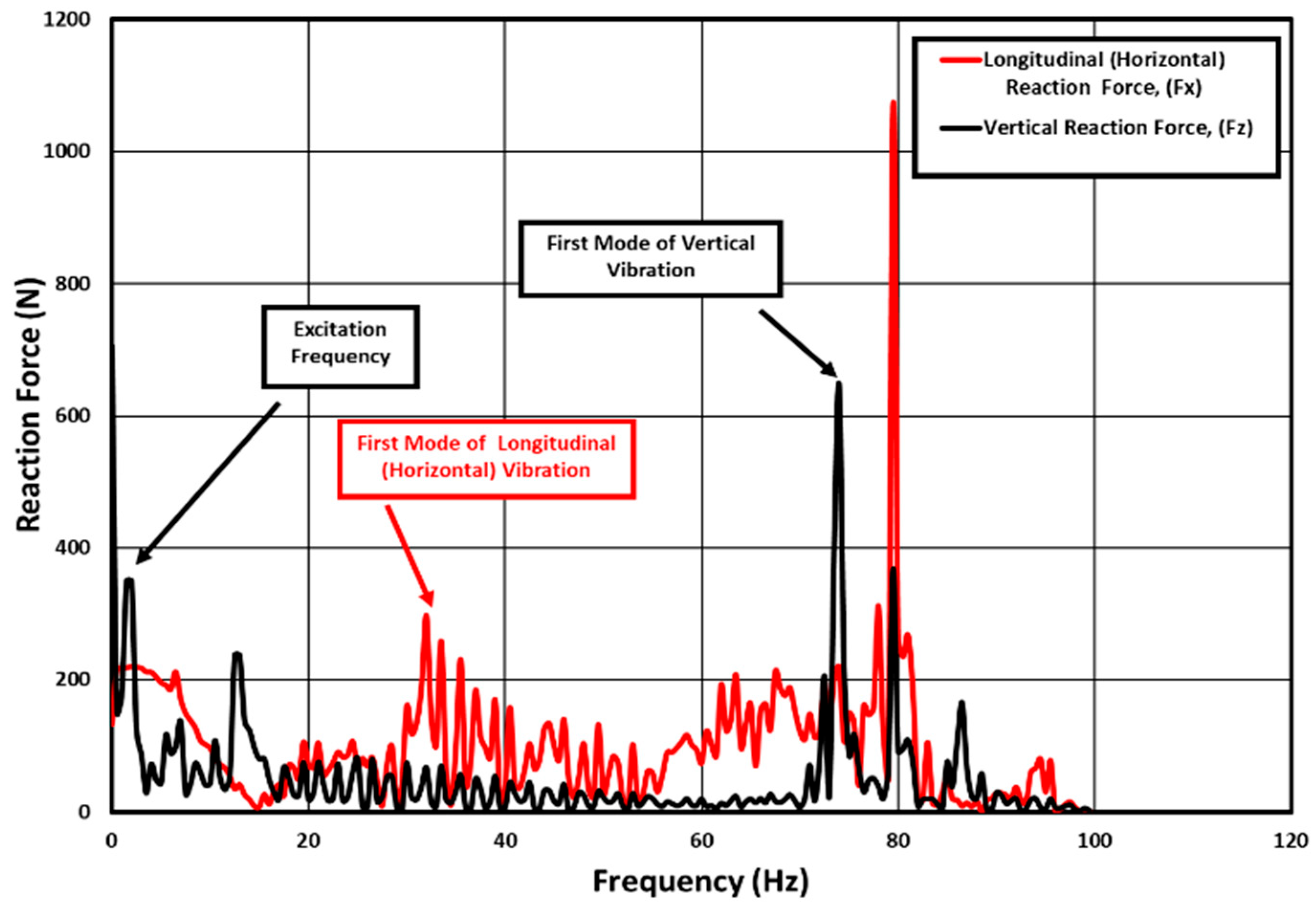
Based on the findings of this research work, it can be concluded that the increase in inflation pressure results in the reduction of static tire footprint areas. Moreover, the footprint test showed that higher deflection of the tread blocks occurs at a higher vertical load, which resulted in a higher footprint contact area. Therefore, it is recommended to design an optimized tire tread pattern that maintains a stable footprint area under various loading conditions. Furthermore, according to the frequency analysis, it was observed that the vertical first mode of vibration occurred at 74 Hz, while the longitudinal first mode of frequency was 32 Hz, which is in good agreement with previously measured data. In addition, it can be concluded that the sidewall damping coefficient is directly affected by the tire inflation pressure, and increasing inflation pressure dramatically gives rise to the full sidewall damping coefficient. However, the vertical load is less effective for changes in the sidewall damping coefficient.

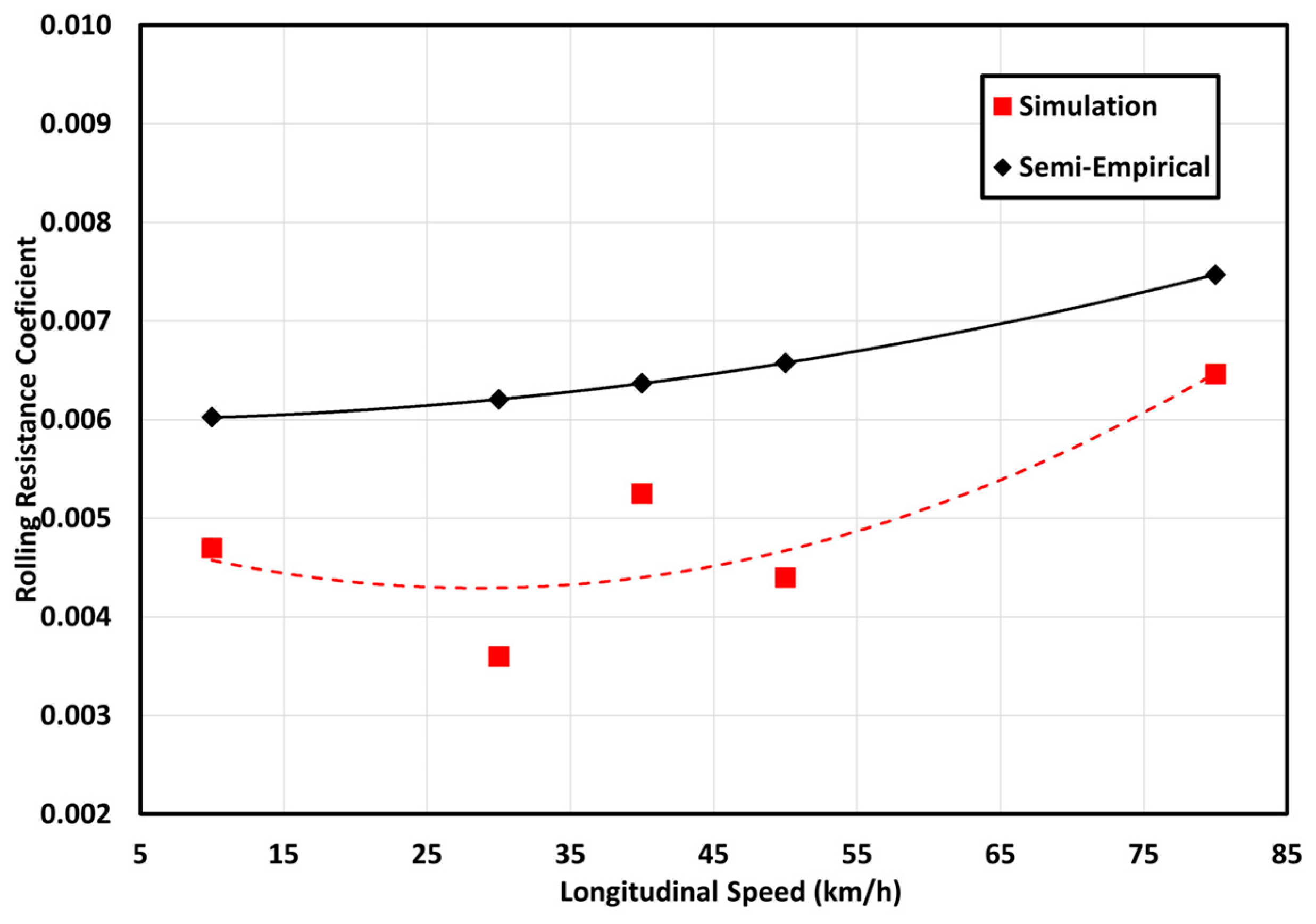
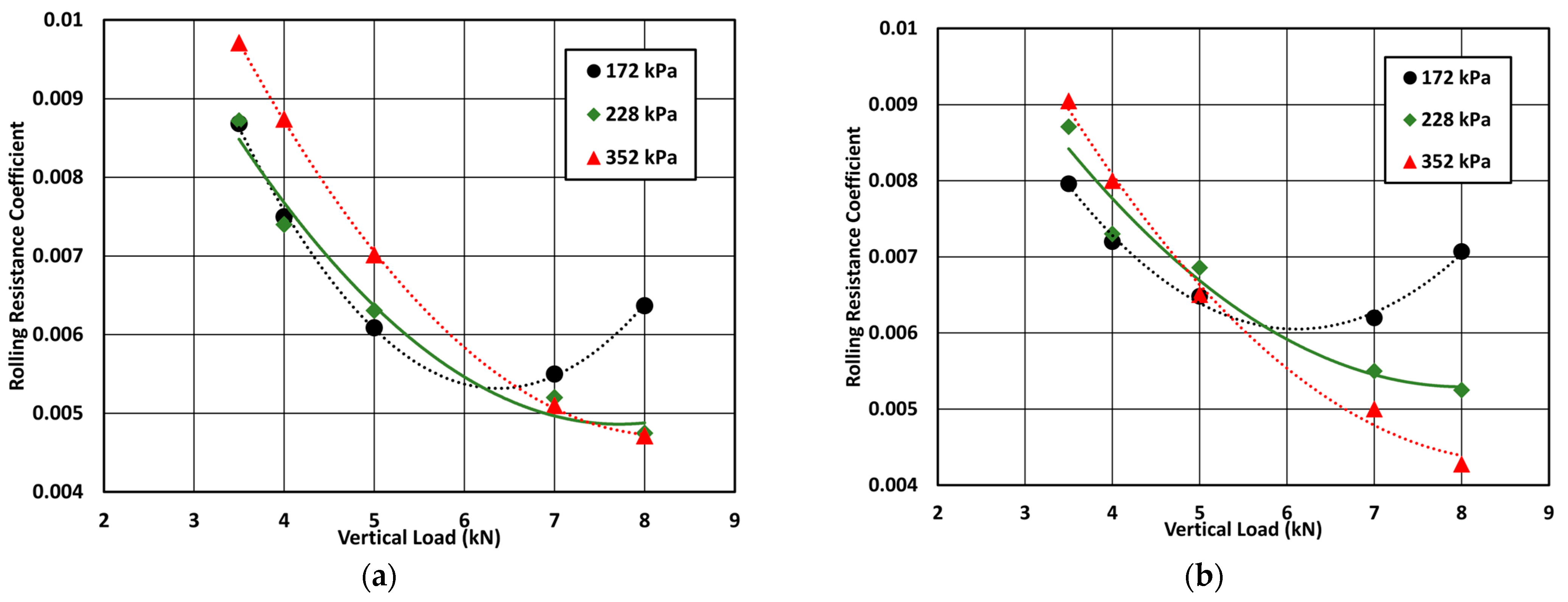
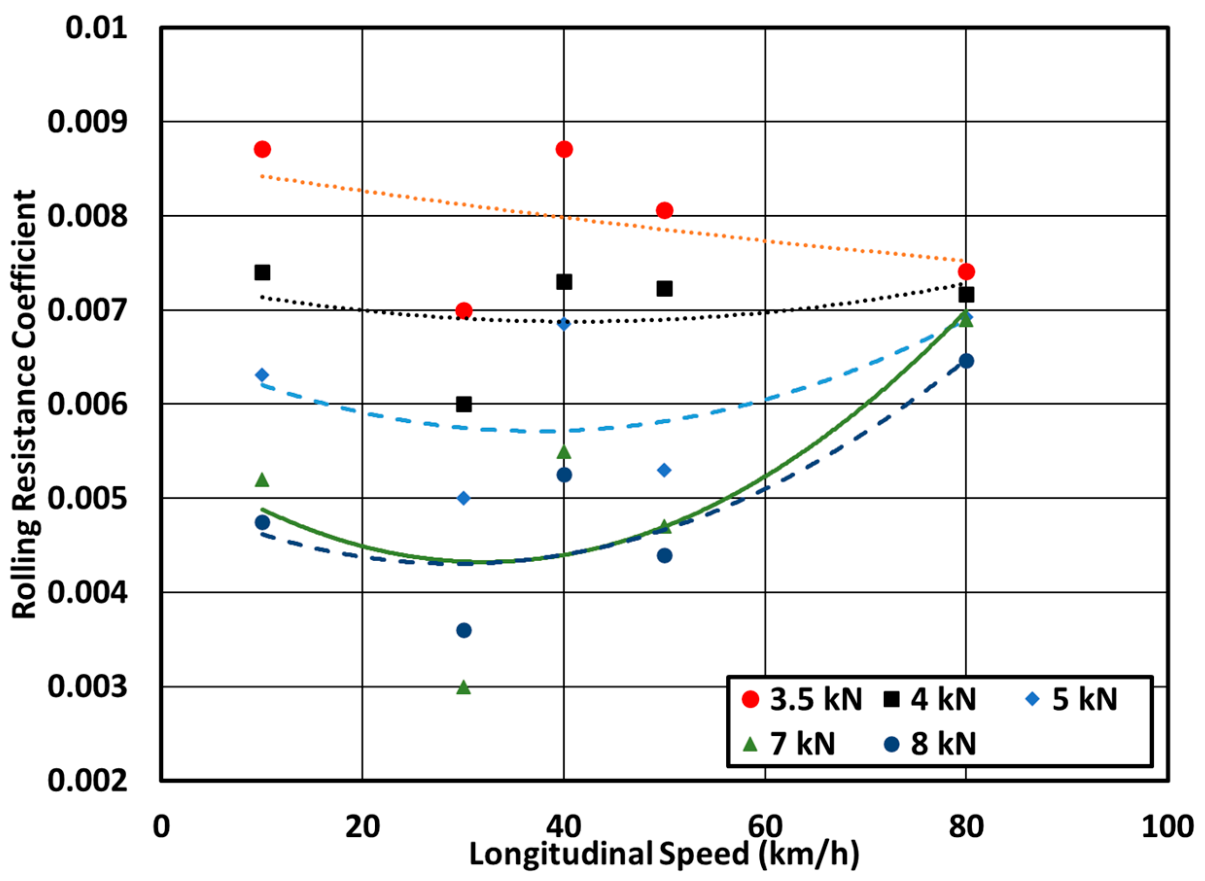
Based on the rolling resistance analysis performed, it was concluded that the vertical load has the largest effect on the rolling resistance coefficient. As the vertical load increases, the rolling resistance coefficient decreases at all ranges of inflation pressures and speeds. Furthermore, as the tire speed increases, the rolling resistance coefficient increases as well; this phenomenon was noticed significantly at higher vertical loads. This research will further continue to investigate the effect of tire rubber compound material on the tire–road interaction characteristics.

References

1. Zorowski, C. Mathematical prediction of dynamic tire behavior. Tire Sci. Technol. 1973, 1, 99–117. [Google Scholar] [CrossRef]
2. Ridha, R. Analysis for tire mold design. Tire Sci. Technol. 1974, 2, 195–210. [Google Scholar] [CrossRef]
3. Kennedy, R.; Padovan, J. Finite Element Analysis of a Steady-State Rotating Tire Subjected to Point Load or Ground Contact. Tire Sci. Technol. 1987, 15, 243–260. [Google Scholar] [CrossRef]
4. Shiraishi, M.; Yoshinaga, H.; Miyori, A.; Takahashi, E. Simulation of dynamically rolling tire. Tire Sci. Technol. 2000, 28, 264–276. [Google Scholar] [CrossRef]
5. Kabe, K.; Koishi, M. Tire cornering simulation using finite element analysis. J. Appl. Polym. Sci. 2000, 78, 1566–1572. [Google Scholar] [CrossRef]
6. Ghoreishy, M. Steady state rolling analysis of a radial tyre: Comparison with experimental results. Proc. Inst. Mech. Eng. Part D J. Automob. Eng. 2006, 220, 713–721. [Google Scholar] [CrossRef]
7. Chae, S. Nonlinear Finite Element Modeling and Analysis of a Truck Tire. Ph.D. Thesis, Pennsylvania State University, State College, PA, USA, 2006. [Google Scholar]
8. Krmela, J. The Computational Modelling of Tire. Recent 2009, 10, 333–336. [Google Scholar]
9. Lardner, K.L.; El-GIndy, M.; Oijer, F.; Johansson, I.; Philipps, D. Determining the Vertical and Longitudinal First Mode of Vibration of a Wide Base FEA Truck Tire; SAE Technical Paper 0148-7191; SAE International: Warrendale, PA, USA, 2016. [Google Scholar]
10. Nussbaumer, H.J.; Nussbaumer, H.J. The Fast Fourier Transform; Springer: Berlin/Heidelberg, Germany, 1982. [Google Scholar]
11. MathWorks. FAst Fourier Transform (FFT). Available online: https://www.mathworks.com/discovery/fft.html (accessed on 25 December 2023).
12. Krmela, J. Tire Casings and Their Material Characteristics for Computational Modeling: Scientific Monograph; Oficyna Wydawnicza Stowarzyszenia Menadżerów Jakości i Produkcji: Częstochowa, Poland, 2017. [Google Scholar]
13. Rafei, M.; Ghoreishy, M.H.R.; Naderi, G. Thermo-mechanical coupled finite element simulation of tire cornering characteristics—Effect of complex material models and friction law. Math. Comput. Simul. 2018, 144, 35–51. [Google Scholar] [CrossRef]
14. El-Sayegh, Z.; El-Gindy, M. Cornering characteristics of a truck tire on wet surface using finite element analysis and smoothed-particle hydrodynamics. Int. J. Dyn. Control 2018, 6, 1567–1576. [Google Scholar] [CrossRef]
15. Krmela, J. Experiments and Computational Modelling of Tires Textbooks for University Students; Trenčianska Univerzita Alexandra Dubčeka v Trenčíne: Trenčín, Slovakia, 2021; ISBN 978-80-270-9020-4. [Google Scholar]
16. El-Sayegh, Z.; El-Gindy, M.; Johansson, I.; Öijer, F. Development and validation of off-road tire-gravelly soil interaction using advanced computational techniques. J. Terramech. 2020, 91, 45–51. [Google Scholar] [CrossRef]
17. Ali, S.N. Rolling Resistance Estimation for PCR Tyre Design Using the Finite Element Method. In Finite Element Methods and Their Applications; IntechOpen: London, UK, 2020. [Google Scholar]
18. Gao, X.; Xiong, Y.; Liu, W.; Zhuang, Y. Modeling and experimental study of tire deformation characteristics under high-speed rolling condition. Polym. Test. 2021, 99, 107052. [Google Scholar] [CrossRef]
19. Phromjan, J.; Suvanjumrat, C. Development of solid tire model for finite element analysis of compressive loading. Songklanakarin J. Sci. Technol. 2021, 43, 229–236. [Google Scholar]
20. Király, T.; Primusz, P.; Tóth, C. Simulation of Static Tyre–Pavement Interaction Using Two FE Models of Different Complexity. Appl. Sci. 2022, 12, 2388. [Google Scholar] [CrossRef]
21. Lu, D.; Yang, W.; Wu, H.; Zhou, T. Research on simplified tire finite element modeling and simulation method. Proc. Inst. Mech. Eng. Part D J. Automob. Eng. 2023. [Google Scholar] [CrossRef]
22. Fathi, H.; Khosravi, M.; El-Sayegh, Z.; El-Gindy, M. An Advancement in Truck-Tire–Road Interaction Using the Finite Element Analysis. Mathematics 2023, 11, 2462. [Google Scholar] [CrossRef]
23. Continental. Available online: https://continentaltire.com/tires/crosscontact-lx-sport (accessed on 25 December 2023).
24. Haug, E. Finite element analysis of nonlinear membrane structures. In Proceedings of the IASS Pacific Symposium PartII on Tension Structures and Space Frames; University of California: Berkeley, CA, USA, 1972; pp. 165–176. [Google Scholar]
25. Group, E. Pam-Crash Theory Notes Manual; PAM System International: Joliet, IL, USA, 2000. [Google Scholar]
26. Rivlin, R.S. Large elastic deformations of isotropic materials IV. Further developments of the general theory. Philos. Trans. R. Soc. Lond. Ser. A Math. Phys. Sci. 1948, 241, 379–397. [Google Scholar]
27. Rivlin, R.S.; Saunders, D. Large elastic deformations of isotropic materials VII. Experiments on the deformation of rubber. Philos. Trans. R. Soc. Lond. Ser. A Math. Phys. Sci. 1951, 243, 251–288. [Google Scholar]
28. Chang, Y.-p.D. Nonlinear FEA Rotating Tire Modeling for Transient Response Simulations; The Pennsylvania State University: State College, PA, USA, 2002. [Google Scholar]
29. KuliKowsKi, K.; Szpica, D. Determination of directional stiffnesses of vehicles’ tires under a static load operation. Eksploat. I Niezawodn. 2014, 16, 66–72. [Google Scholar]
30. Sun, P.; Feng, G.; Zhou, S.; Qiu, C.; Fan, J. Experimental analysis of radial tire stiffness and grounding characteristics. IOP Conf. Ser. Mater. Sci. Eng. 2019, 677, 022111. [Google Scholar] [CrossRef]
31. Dudziak, M.; Lewandowski, A.; Waluś, K.J. Static tests the stiffness of car tires. IOP Conf. Ser. Mater. Sci. Eng. 2020, 776, 012071. [Google Scholar] [CrossRef]
32. ISO 20908:2023; Tyre Sound Emission Test—Methods of Drum. ISO: Geneva, Switzerland, 2023. Available online: https://www.iso.org/standard/79096.html (accessed on 25 December 2023).
33. ISO 13326:1998(en); Test Methods for Measuring Tyre Uniformity. ISO: Geneva, Switzerland, 1998. Available online: https://www.iso.org/standard/21715.html (accessed on 25 December 2023).
34. ISO 28580:2018; Passenger Car, Truck and Bus Tyre Rolling Resistance Measurement Method: Single Point Test and Correlation of Measurement Results. ISO: Geneva, Switzerland, 2018.
35. Ejsmont, J.; Taryma, S.; Ronowski, G.; Swieczko-Zurek, B. Influence of load and inflation pressure on the tyre rolling resistance. Int. J. Automot. Technol. 2016, 17, 237–244. [Google Scholar] [CrossRef]
36. Taghavifar, H.; Mardani, A. Investigating the effect of velocity, inflation pressure, and vertical load on rolling resistance of a radial ply tire. J. Terramech. 2013, 50, 99–106. [Google Scholar] [CrossRef]
37. Grappe, F.; Candau, R.; Barbier, B.; Hoffman, M.; Belli, A.; Rouillon, J.-D. Influence of tyre pressure and vertical load on coefficient of rolling resistance and simulated cycling performance. Ergonomics 1999, 42, 1361–1371. [Google Scholar] [CrossRef]
38. Redrouthu, B.M.; Das, S. Tyre Modelling for Rolling Resistance. Master’s Thesis, Chalmers University of Technology, Gothenburg, Sweden, 2014. [Google Scholar]
39. Wong, J.Y. Theory of Ground Vehicles; John Wiley & Sons: Hoboken, NJ, USA, 2022. [Google Scholar]
Figure 1. Membrane element concepts in Pam-Crash [15].
Vehicles 06 00016 g001
Figure 2. FEA 235/55R19 tire in Pam-Crash. (a) FEA full rotated tire; (b) cross-section of the tire.
Vehicles 06 00016 g002
Figure 3. Aluminum wheel assembly FEA model in Pam-Crash software.
Vehicles 06 00016 g003
Figure 4. Contact definition in Pam-Crash, perforation, and penetration [25].
Vehicles 06 00016 g004
Figure 5. Appended FEA 235/55R19 tire–rigid road model in Pam-Crash.
Vehicles 06 00016 g005
Figure 6. The nodal displacement contour at footprint test for nominal inflation pressure and nominal load.
Vehicles 06 00016 g006
Figure 7. Tire drum-cleat test setup for the FEA passenger car tire model.
Vehicles 06 00016 g007
Figure 8. Frequency analysis of a 235/55R19 tire at 228 kPa inflation pressure and 5 kN vertical load.
Vehicles 06 00016 g008
Figure 9. Tire RRC as a function of vertical load at three inflation pressures and longitudinal speeds: (a) 10 km/h longitudinal speed; (b) 40 km/h longitudinal speed.
Vehicles 06 00016 g009
Figure 10. Effect of longitudinal speed on the tire’s rolling resistance coefficient at different vertical loads and a nominal inflation pressure of 228 kPa.
Vehicles 06 00016 g010
Figure 11. RRC as a function of five longitudinal speeds (10 km/h, 30 km/h, 40 km/h, 50 km/h, and 80 km/h) at 228 kPa inflation pressures and an 8 kN vertical load.
Vehicles 06 00016 g011