Abstract
Detecting drivers’ cognitive states poses a substantial challenge. In this context, cognitive driving anomalies have generally been regarded as stochastic disturbances. To the best of the author’s knowledge, existing safety studies in the realm of human Driving Anomaly Detection (DAD) utilizing vehicle trajectories have predominantly been conducted at an aggregate level, relying on data aggregated from multiple drivers or vehicles. However, to gain a more nuanced understanding of driving behavior at the individual level, a more detailed and granular approach is essential. To bridge this gap, we developed a Data Anomaly Detection (DAD) model designed to assess a driver’s cognitive abnormal driving status at the individual level, relying solely on Basic Safety Message (BSM) data. Our DAD model comprises both online and offline components, each of which analyzes historical and real-time Basic Safety Messages (BSMs) sourced from connected vehicles (CVs). The training data for the DAD model consist of historical BSMs collected from a specific CV over the course of a month, while the testing data comprise real-time BSMs collected at the scene. By shifting our focus from aggregate-level analysis to individual-level analysis, we believe that the DAD model can significantly contribute to a more comprehensive comprehension of driving behavior. Furthermore, when combined with a Conflict Identification (CIM) model, the DAD model has the potential to enhance the effectiveness of Advanced Driver Assistance Systems (ADAS), particularly in terms of crash avoidance capabilities. It is important to note that this paper is part of our broader research initiative titled “Automatic Safety Diagnosis in the Connected Vehicle Environment”, which has received funding from the Southeastern Transportation Research, Innovation, Development, and Education Center.
1. Introduction
The realm of driving constitutes a complex and intricately interconnected system, where the occurrence of a crash typically arises from a malfunction within one or more of its constituent elements. In the context of safety analysis, Haddon [1] has classified these elements into vehicle-related factors, road-related factors, and human-related factors. Among these factors contributing to crashes, the human element emerges as the most prevalent, responsible for over 90% of all recorded accidents [2].
The study of driver behavior has been the subject of extensive research within the domains of traffic simulation and vehicle control systems. Some investigations have portrayed the driver as an optimized feedback controller, actively pursuing specific control objectives like maintaining a safe following distance [3], planning optimal routes [4], or optimizing an electric vehicle’s battery energy consumption. In the energy management system of Plug-in Hybrid Electric Busses, the anticipation of travel patterns was predicted for various factors, including the speed and acceleration of the buses as well as the type of road [5]. This prediction aimed to align driving behavior with the current road conditions as accurately as possible. Furthermore, a hardware-in-the-loop (HIL) platform was established to facilitate an energy consumption strategy that takes into account the awareness of driving behavior [6]. Conversely, alternative research approaches have portrayed drivers as autonomous systems, often subjected to stochastic disturbances [7,8,9,10]. Nonetheless, a noteworthy gap persists between predictive models of driving behavior and the reality of human drivers on the road. Human driving is fundamentally steered by the conscious and subconscious processes of the human brain, leading to instantaneous decision making and actions within the dynamic driving environment. While it is feasible to simulate undisturbed human driving using optimization techniques, the modeling of disturbed or distracted human driving, which involves inherently random processes, poses significant challenges and remains less amenable to accurate representation.
Distracted or impaired driving behavior significantly contributes to the occurrence of accidents as it impairs a driver’s ability to perform effectively behind the wheel. Liang introduced a classification system for driving distractions in 2010, categorizing them into visual distractions and cognitive distractions [11]. Visual distractions involve the driver taking their eyes off the road, a behavior that can be observed directly. Conversely, cognitive distractions relate to a driver’s mental state and their lack of focus on driving, which are more difficult to detect since the signs of cognitive distraction are not readily observable and may vary among individuals.
The Second Strategic Highway Research Program (SHRP2) Naturalistic Driving Study (NDS) stands out as the most extensive investigation into distracted driving. This study collected a wealth of data, including information on vehicle speed, acceleration, braking, all aspects of vehicle controls, lane positioning, forward radar, and video footage capturing views both in front and behind a vehicle and of the driver’s face and hands [12]. In 2020, a distracted driving experiment was carried out in Baltimore, exposing drivers to various distractions such as hands-free calling, hand-held calling, voice commands, texting, adjusting clothing, and eating/drinking. Notably, among these distractions, only hands-free calling was classified as a cognitive distraction [13]. While numerous studies have utilized the NDS data to explore visual distractions, cognitive distraction has received relatively less attention. Quantifying the intricate relationship between a driver’s cognitive state and observable signs of distraction remains a significant challenge [14]. It is important to highlight that a study focusing on investigating cognitive distraction was conducted in a controlled environment designed to simulate cannabis intoxication and impaired driving. The findings from this study revealed that the participants showed delayed speed reduction when they encountered changes in traffic signals [15]. Nonetheless, it is essential to recognize that even though driving decisions are made in the heat of the moment, there are underlying psychological factors that precede a driver’s abnormal behavior before reaching the scene of a crash [16].
Anomaly detection is a data-mining technique employed to identify events that diverge from the norm and do not adhere to a predefined standard behavior [17]. When applied to the domain of driving, it is referred to as Driving Anomaly Detection (DAD), which aims to pinpoint instances of driving anomalies (DAs). The methods used for DAD can be categorized based on how DAs are defined, and there are three primary approaches in this regard.
Firstly, DAs can be defined based on common sense, identifying specific states and behaviors that are likely to lead to accidents, such as aggressiveness, drowsiness, and impaired driving [18]. Secondly, since most drivers typically adhere to traffic regulations, any driving maneuver that deviates from the statistical majority is considered abnormal. Therefore, DAs are defined as departures from the statistical norm. Thirdly, each driver has their own unique driving pattern or style. For most drivers, accidents are infrequent events, and they can drive safely for extended periods. Driving is a complex behavior, and each driver develops their own habitual way of driving safely. In this context, not adhering to one’s established driving pattern can also be regarded as a driving anomaly [19,20].
In the context of the first definition of DAs, DAD involves the monitoring of a driver’s physical attributes, such as via breath analysis through in-vehicle alcohol sensors and the observation of facial and body movements using cameras and image-processing technology. These methods, while straightforward, come with several drawbacks, including high device costs, technical limitations, and privacy concerns [21]. Conversely, based on the second definition of DAs, many DAD systems utilize socio-economic (SE) data such as age, gender, and income level, among others. SE factors have been presumed to have psychological influences on driving behavior [22] and have been statistically linked to the occurrence of accidents. These SE methods have found widespread adoption by automobile manufacturers and insurance companies for identifying high-risk drivers due to the ease and cost-effectiveness of obtaining such measurements [23].
Additionally, under the second DA definition, trajectory data, which represent patterns in driving maneuvers, have been employed. For instance, highway patrol officers monitor vehicle trajectories to identify traffic violations. The term “aggressive driving” was used by the National Highway Traffic Safety Administration to categorize actions that significantly exceeded the norms of safe driving behavior. However, the challenge lay in defining these “norms” theoretically, primarily because individual driving patterns vary greatly [24]. What constituted the norm for a cautious driver might not align with that of an assertive driver. Consequently, in non-administrative safety research, the term “driving volatility” replaced “driving aggression”, as it offered a more objective and measurable descriptor for instantaneous driving decisions [25].
Within the context of driver behavior analysis, researchers have explored various parameters embedded in driving trajectories, including speed, acceleration [25], and jerks [26], which have been identified and chosen as key performance indicators (KPIs) for quantifying driving volatility. However, employing speed as a direct KPI for Driving Anomaly Detection (DAD) has been considered simplistic, as it is influenced by contextual factors such as speed limits [27]. One straightforward approach to addressing this was to consider higher maximum speeds, as they are linked to drivers with a higher number of recorded accidents [25]. Acceleration also emerged as an indicator associated with risky driving behavior. Threshold values for abnormal acceleration were established, with 1.47 m/s2 denoting aggressive acceleration and 2.28 m/s2 signifying extremely aggressive acceleration [28], while [29] defined the range of 0.85 to 1.10 m/s2 as aggressive acceleration. Nevertheless, a consensus on these values remained elusive due to their sensitivity to contextual factors [30].
In the pursuit of a comprehensive understanding of driver behavior, researchers have conducted investigations into how acceleration patterns changed concerning both speed [31] and time [32]. These examinations revealed that accelerations exhibited variability depending on a vehicle’s speed, and alterations in acceleration did not consistently align across different directional axes. Consequently, researchers introduced a set of multivariate Key Performance Indicators (KPIs) designed to encompass both longitudinal and lateral accelerations within various speed ranges [33].
While rule-based methods, as exemplified by Martinez [34], offer simplicity and efficiency, they possess inherent limitations when it comes to accommodating the diverse driving behaviors exhibited by individuals. This prompted the widespread adoption of DAD at the individual level, also known as agent-based DAD, as defined in the third DA definition. The rationale behind focusing on the individual level stemmed from the expectation of increased accuracy compared to aggregate-level approaches. For instance, if a typically fast driver were compelled to drive at a slower pace, they might become overly relaxed and pay less attention to driving than necessary for ensuring safety. Conversely, drivers are generally more skilled and safer when adhering to their own established driving patterns. In contrast, aggregate-level analysis takes an average across all drivers, potentially smoothing out individual characteristics. The advantage of individual-level analysis over aggregate-level analysis also lies in its ability to be tailored and fine-tuned to match the specific characteristics of each driver.
A driver profile refers to a group of drivers who share similar driving behaviors and traits, while a driving pattern relates to a specific driving behavior that is consistently observed for one or more drivers [35]. However, there has been a lack of systematic exploration into the characteristics, insights, and added value of various methods and analysis scales for recognizing driver profiles and driving patterns [36]. The existing literature primarily focuses on the collective level, with only a few studies employing adaptive fuzzy algorithms to identify driving patterns for each individual driving instance within a trip in order to construct a composite profile for an entire trip [37]. There is a noticeable absence of individual-level recognition for driving anomalies.
Despite its notable advantages, the utilization of vehicle trajectories for DAD at the individual driver level has not been documented extensively in the existing literature. One possible explanation for this scarcity could be the substantial computational power required, which might not have been readily available. However, a more plausible reason lies in the perceived complexity of modeling driving behavior. Driving necessitates the coordinated functioning of four pairs of brain lobes—occipital, temporal, parietal, and frontal—involving both conscious and subconscious cognitive processes [38]. Driving represents a sequence of actions driven by spontaneous decisions originating from the human brain, which continuously responds to instantaneous alterations in the surrounding environment, including factors such as nearby vehicles, road conditions, geometry, and weather [30]. A comprehensive study of DAD would inherently be multidisciplinary, requiring the collaboration of experts not only in transportation and computer science but also in fields like neurology and cognitive science [39]. Nonetheless, as a practical shortcut to fully launching a comprehensive study, examining vehicle trajectories could serve as an initial step. This approach involves transitioning from highway patrol officers visually monitoring vehicle trajectories to identify traffic violations to implementing in-vehicle computers equipped with computational models for detecting driving anomalies.
Essentially, a DAD system can be seen as a model for identifying anomalies or outliers, a concept commonly used in data science. Outliers are data points that markedly deviate from the majority of a set of data. In the realm of machine learning (ML) programs, outlier detection (OD) serves as an initial step in the data-cleaning process. Interestingly, OD has also evolved into a field of developing ML algorithms in its own right. OD tasks typically fall under the umbrella of unsupervised ML because data often lack labels, particularly since outliers are typically rare occurrences [40]. This absence of labels poses a challenge in quantifying deviation through statistical and mathematical measures, leading to significant research efforts and the development of numerous OD algorithms in various programming languages.
Fundamentally, unsurprised OD algorithms can be categorized into several basic types, including Angle-Based Outlier Detection (ABOD) [41], Cluster-based Local Outlier Factor (CBLOF) [42], Histogram-based Outlier Detection (HBOS) [35], Isolation Forest [43], and K-Nearest Neighbors (KNN) [44] algorithms. These diverse OD algorithms employ distinct approaches to measure deviations, and the corresponding datasets vary in terms of dimensions and features, while user interests also differ. Consequently, determining a universally superior OD ML algorithm is challenging, and reaching a consensus is difficult. Consequently, the selection of an appropriate algorithm becomes crucial for effective OD processing. To enhance user convenience, packages have been developed to bundle various OD algorithms together. For instance, the PyOD package aggregates more than forty OD algorithms and has found widespread use in academia and industry, boasting over 10 million downloads [45]. The application domains of OD are extensive and encompass areas such as finance (for credit card fraud detection), healthcare (for the identification of malignant tumors) [46], astronomy (for spacecraft damage detection), cybersecurity (for intrusion detection) [17], and the connected vehicle (CV) environment (for signal intrusion detection) [24].
In fact, the CV project stands out as a valuable data source for conducting OD analyses of driving behavior. Extensive endeavors have been undertaken by both the USDOT (United States Department of Transportation) and automotive manufacturers to drive the development and advocacy of Connected Vehicles (CVs), and Connected and Autonomous Vehicles (CAVs) will gradually be deployed in the coming years as the heart of ITS. The core of the CV project revolves around the Basic Safety Message (BSM), which is alternatively referred to as vehicle-to-everything communications (V2X) or “Here I Am” data messages. As a CV operates on the road, it continuously generates and receives BSMs from nearby CVs and any entities capable of communicating with BSMs. These BSMs are generated within specialized onboard devices (OBDs) designed specifically for Connected Vehicles (CVs). In the transmission phase, these BSMs are broadcasted through low-latency communication devices, either operating on the dedicated 5.9 GHz spectrum at a frequency of 10 Hz [47] or through a 5G network. Nearby CVs and roadside units (RSUs) have the capability to receive these BSMs. The effective transmitting range of BSMs typically ranges from 300 m to 1000 m. The format of a BSM was standardized by the Society of Automotive Engineers J2735, which is the Dedicated Short-Range Communications (DSRC) Message Set Dictionary. A typical BSM contains information such as vehicle ID, epoch time, GPS location, speed, acceleration, yaw rate, and supplementary details [47]. It is important to note that BSMs are considered disposable and are not reused.
A notable barrier preventing the widespread acceptance of CAVs pertains to safety. When it comes to assessing the traffic safety of a CAV, the majority of current studies focus on quantifying driving risk using surrogate safety measures (SSMs) [48]. At the moment, CAV safety heavily relies on the surveillance systems and motion detection features embedded within a CAV. However, in the event of a malfunction in a CAV’s surveillance system, safety concerns may arise. To address this safety issue, an alternative method consists of transmitting notifications regarding potential near-crash scenarios to drivers through an alternate communication channel. This can be effectively achieved by analyzing the vehicle trajectories provided in BSMs within a CV environment [49].
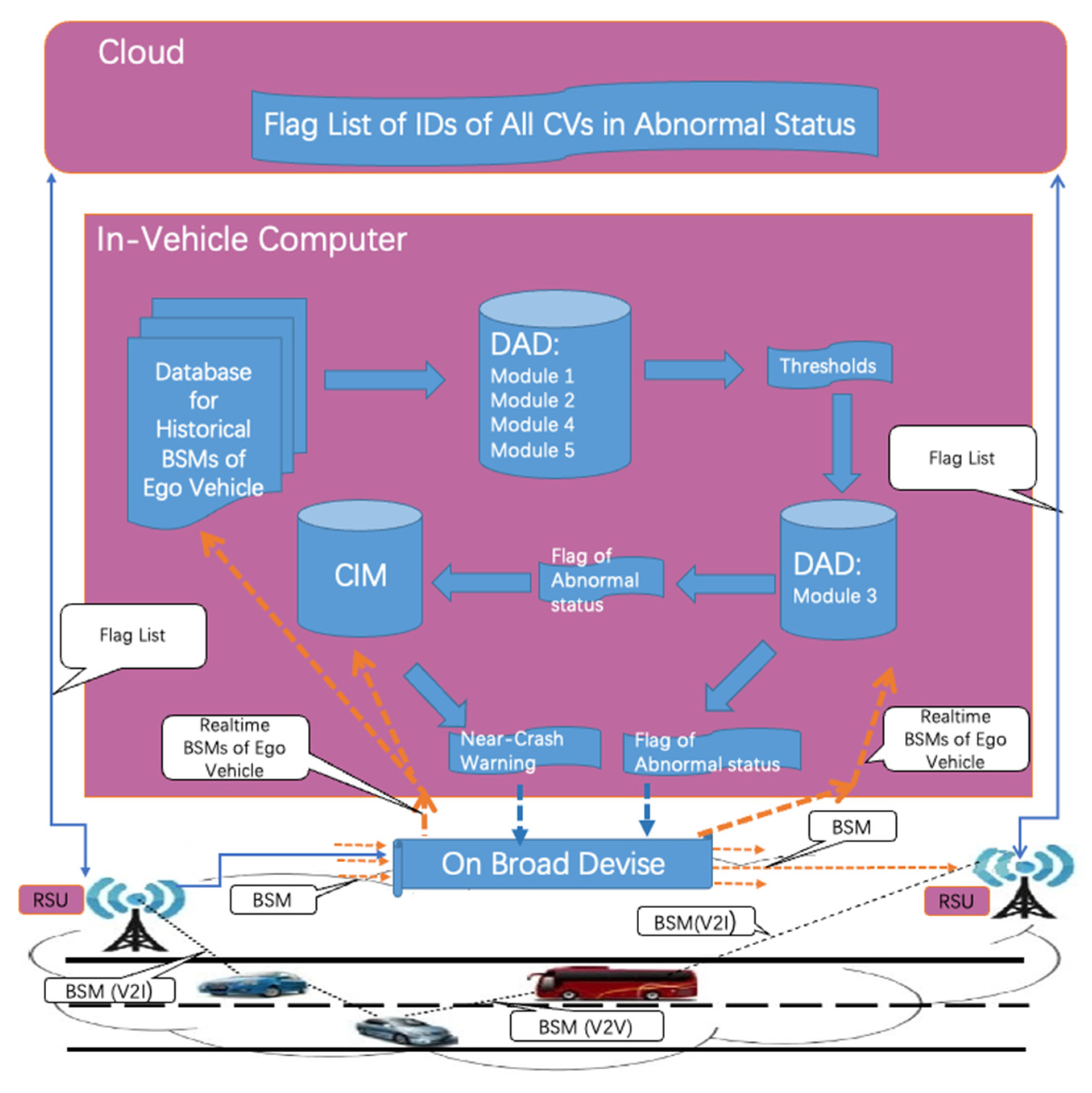
Our research project, titled “Automated Safety Diagnosis in the CV Environment”, was initiated with the goal of creating an individual-level near-crash warning system that relies exclusively on Basic Safety Messages (BSMs). We define a near-crash as a conflict [49] in which at least one of the vehicles involved exhibits abnormal driving behavior. As shown in the conceptual architecture of our research, depicted in Figure 1, the system comprises several components: a Driver Anomaly Detection (DAD) component, a Conflict Identification Model (CIM) [49], a cloud subsystem, and the data pathways connecting them. Within each Connected Vehicle (CV), the In-vehicle Computer (IVC) collects its own historical BSMs and employs the DAD to establish thresholds that differentiate between normal and abnormal driving behaviors. The IVC also gathers real-time BSMs from its own vehicle and nearby CVs, utilizing the CIM to assess the presence of conflicts betweendthe ego vehicle and other CVs as well as examining its own driving status. If an anomaly event is detected, a notification is transmitted to the cloud. The cloud subsystem maintains a flag list that contains information about all abnormal CVs within its region and continuously shares this list with all CVs within the service area.
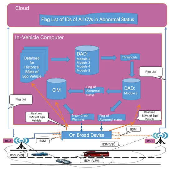
Figure 1.
The conceptual architecture of the near-crash warning system.
Our DAD system demonstrates adaptability by incorporating both historical BSMs and real-time BSMs. It leverages historical BSMs to generate thresholds while using real-time BSMs to evaluate whether the ego vehicle’s driving behavior deviates from the norm. The adaptability of this system stems from the continuous updating of historical BSMs. The system demonstrates its practicality by integrating into current driving warning systems an near crash warning tool that using BSMs as exclusive data source; in contrast, the prevailing warning tools depend on cameras and sensors. This paper provides an overview of our DAD model. The conflict and CIM were introduced in detail in [49].
Some examples of this paper’s noteworthy contributions are as follows:
- (a)
- Pioneering a method for the identification of a near-crash scenario based on TWO specific conditions: a DA and conflict.
- (b)
- Establishing a system to exam DAs at an individual level.
- (c)
- Demonstrating the innovative use of the information within BSM by dividing it into two modules: one harnessing time-related information in the DAD component and the other making effective use of spatial attributes, particularly coordinates, within the CIM component. This approach offers a fresh perspective on handling BSM data.
- (d)
- Introducing an innovative systematic approach that integrates a cloud and the CV environment for the exchange of anomaly CV lists.
2. Materials and Methods
2.1. Data Description
The data used for our study consisted of two datasets: the BSMs from the Safety Pilot Model Deployment (SPMD) data served as our working dataset, and the BSMs from the second Strategic Highway Research Program (SHRP2) of the Naturalistic Driving Study (NDS) were chosen for evaluation data.
2.1.1. SPMD Data
The SPMD project was an integral component of the US Department of Transportation’s Connected Vehicle (CV) program. The SPMD dataset is accessible through the Intelligent Transportation System (ITS) Data Hub, which can be found at its.dot.gov/data/ (accessed on 15 September 2022). For our project, we utilized working data obtained from the field BSM data collected during an SPMD test conducted in Ann Arbor, Michigan, in October 2012. The BSM data were stored in a Comma-Separated Values (CSV) file, denoted as BsmP1, which had a substantial size of 67 gigabytes and contained all the BSMs generated by the 1527 test vehicles involved in the experiment. The original downloaded data file included 19 attributes and encompassed over 500 million records. As part of our data-preprocessing efforts, we filtered out irrelevant attributes, resulting in a refined data file with 11 attributes. These attributes included DevID for vehicle identification, EpochT for timestamp information, and attributes for latitude, longitude, accelerations, heading, and yaw rate. One can find detailed descriptions of these attributes in Table 1. The SPMD dataset does not include any records of incidents, and we did not discover any related incidents elsewhere in our search.

Table 1.
The selected attributes of BSM data.
2.1.2. SHRP2 Data
The Naturalistic Driving Study (NDS) conducted as part of the Second Strategic Highway Research Program (SHRP2) is a research initiative aiming to investigate the influence of driver performance and behavior on traffic safety. The Virginia Tech Transportation Institute (VTTI) plays crucial roles as the technical coordinator and study design contractor for the NDS, and it operates the InSight Data Access Website [50].
On the InSight Data Access Website, one can find a section called the Event Detail Table, which contains a total of 41,530 records documenting various incidents of crashes and near crashes. Each of these records is available online and includes comprehensive information about the events. This information encompasses a video clip capturing the 25 s leading up to an event, detailed data regarding the event itself, and a final narrative description.
From this extensive dataset, we specifically chose 46 crash events and extracted 12,500 trajectories related to both historical trips and those that resulted in crashes from the SHRP2 (Strategic Highway Research Program 2) dataset. Notably, since crashes were infrequent occurrences and the number of instrumented vehicles was limited, we did not acquire any recorded crashes that occurred between these instrumented vehicles. Instead, all the recorded crashes involved an instrumented vehicle colliding with a stationary object, such as a tree, fence, or roadway curb.
To safeguard potentially sensitive or personally identificatory information within the SHRP2 trajectory data, certain restrictions and privacy measures were applied. For example, specific details like the exact GPS coordinates for crash trips, the precise timing of events, and any data that could potentially lead to the identification of a driver were not disclosed. The attributes of the time series data closely resemble those found in the BSM (Basic Safety Message) data, as illustrated in Table 1.
2.2. Methods
The DAD system is structured to allow for the utilization of recent historical BSM data from a CV to establish thresholds. These thresholds are subsequently employed for the purpose of identifying anomalies within real-time BSM data. The DAD process comprises five distinct modules, each serving a specific function: Module 1—Data Preprocessing and Key Performance Indicator (KPI) Selection; Module 2—Learning the Normal Behavior; Module 3—Identifying Outliers; Module 4—Determining Abnormal Driving Events; and Module 5—System Updates. These modules are depicted in Figure 2 for reference.
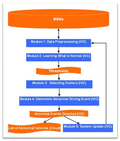
Figure 2.
Flowchart of the DAD model.
2.2.1. Module 1: Data Preprocessing and Selecting KPIs
The fundamental step in constructing a DAD system is gaining a deep understanding of the characteristics of the data it operates on. In the case of BSMs, the data structure resembles discontinuous time series (TS) data. This type of dataset falls under the category of sequence data, where instances are linearly ordered, but it often contains numerous not-available (NA) records. Typically, TS data comprise two main components: (a) Contextual Attributes (CAs), such as timestamps and coordinates, which are essential for establishing the context of each data instance, and (b) Behavioral Attributes (BAs), such as speed and acceleration, which characterize the behavior being observed. Additionally, BSMs are considered spatial data due to their inclusion of coordinates. When treating timestamps as CAs and coordinates as BAs, BSMs exhibit high cardinality. Conversely, if we reverse this perspective and consider coordinates as CAs and time as BAs, BSMs still maintain high cardinality. Furthermore, if both time and coordinates are treated as CAs, the number of potential contexts becomes nearly infinite.
To address this complexity and make the problem more manageable, we propose a strategy of division and specialization, focusing on two distinct sub-problems: time-related and space-related information. Time-related information is leveraged within the DAD component, while spatial attributes, specifically the coordinates, are utilized within the Contextual Information Management (CIM) component. This approach allows us to effectively tackle the challenges presented by the unique characteristics of BSM data.
In the process of visualizing data related to Key Performance Indicators (KPIs) over time, we did not observe any discernible periodic patterns. Furthermore, when subjecting the data to autocorrelation tests (ANOVA), we did not detect any indications of seasonality.
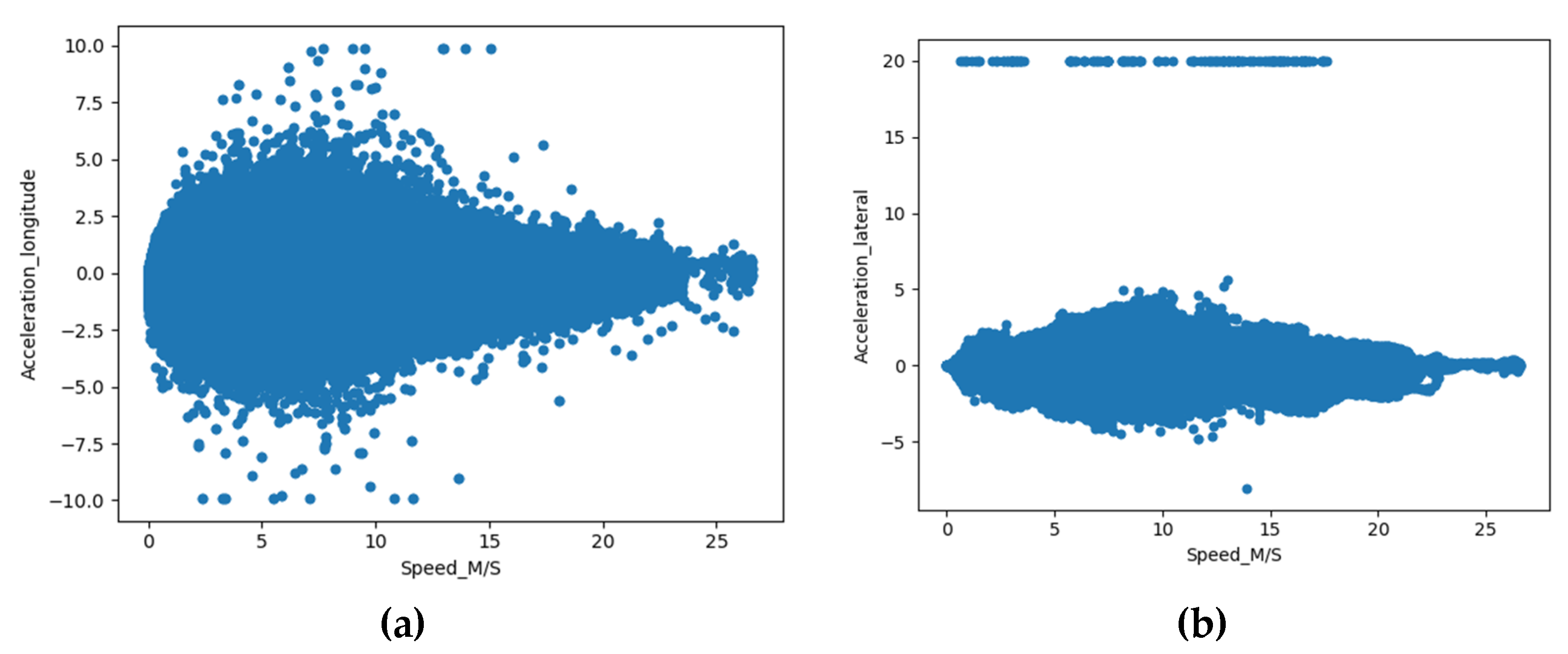
Building upon prior research that highlighted correlations between accelerations and speed, we conducted a thorough analysis of the raw data derived from selected test Connected Vehicles (CVs). Figure 3 illustrates our findings, indicating that the relationship between Acceleration_Longitudinal and Speed, as well as Acceleration Lateral and Speed, displayed a distribution that tended to cluster around a central axis. These observations align with the conclusions drawn in previous studies conducted by Liu [33,51]. Given that KPIs like longitudinal acceleration, lateral acceleration, longitudinal jerk, and lateral jerk have been established to coincide with abnormal driving conditions according to prior research [25,26,31], we opted to use speed as a contextual variable instead of time. It is important to highlight that determining threshold values for differentiating between normal and abnormal conditions is context-specific and lacks consensus in the existing literature, as noted by [30]. Consequently, our approach involved treating these thresholds as adjustable parameters rather than fixed values. This adaptation allowed us to address the contextual variability and sensitivity associated with these threshold settings.

Figure 3.
Scatter plots of acceleration versus speed. (a) Acceleration_ longitudinal versus speed. (b) Acceleration_ lateral versus speed.
In addition, we have categorized the Key Performance Indicators (KPIs) into positive and negative groups. For instance, we distinguish between Acceleration—Longitudi nal_Positive and Acceleration—Longitudinal_Negative, as they correspond to distinct driver actions, such as accelerating or braking, and may exhibit distinct patterns. Consequently, we established a total of eight KPIs Accordingly.
2.2.2. Module 2: Learning What Is Normal
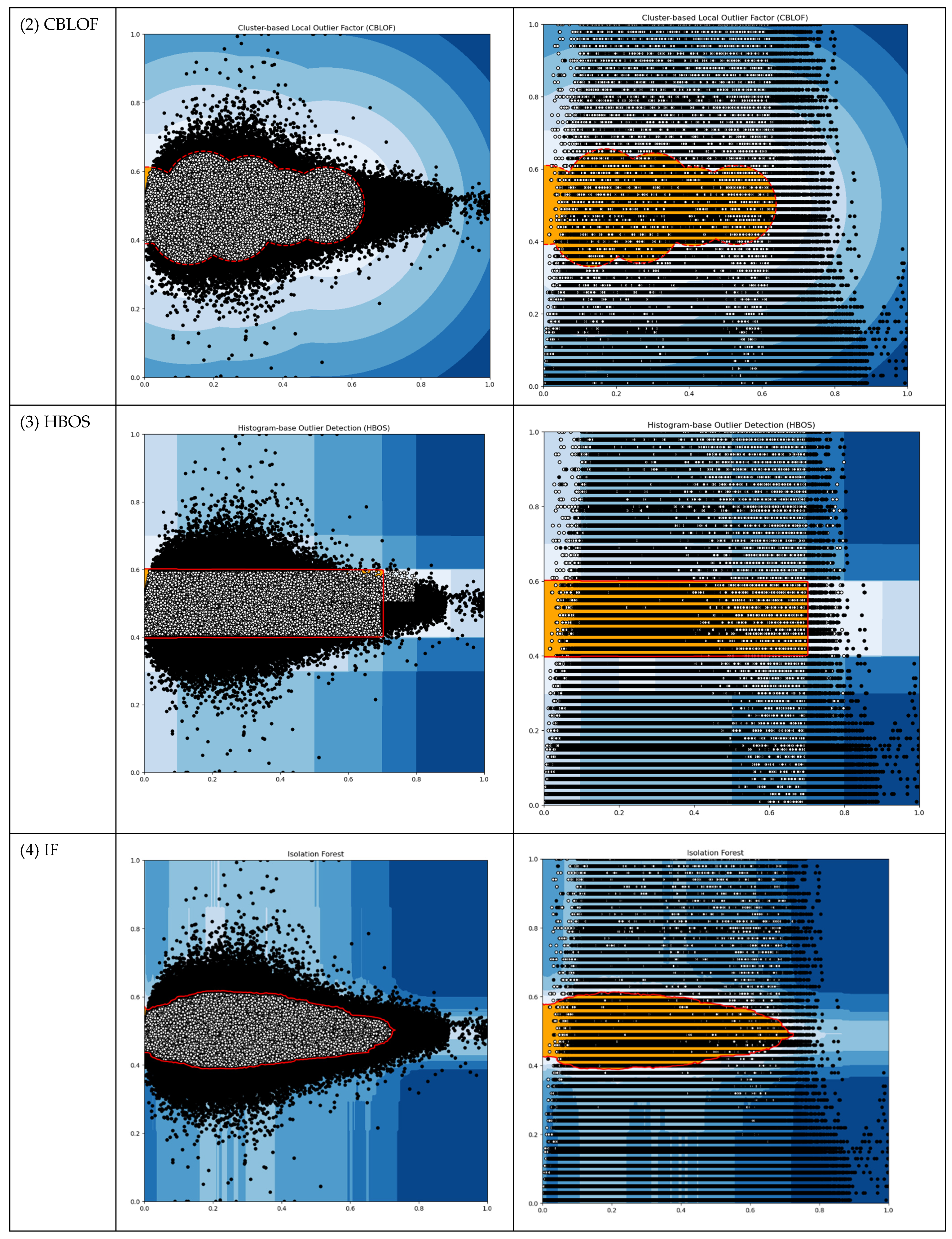
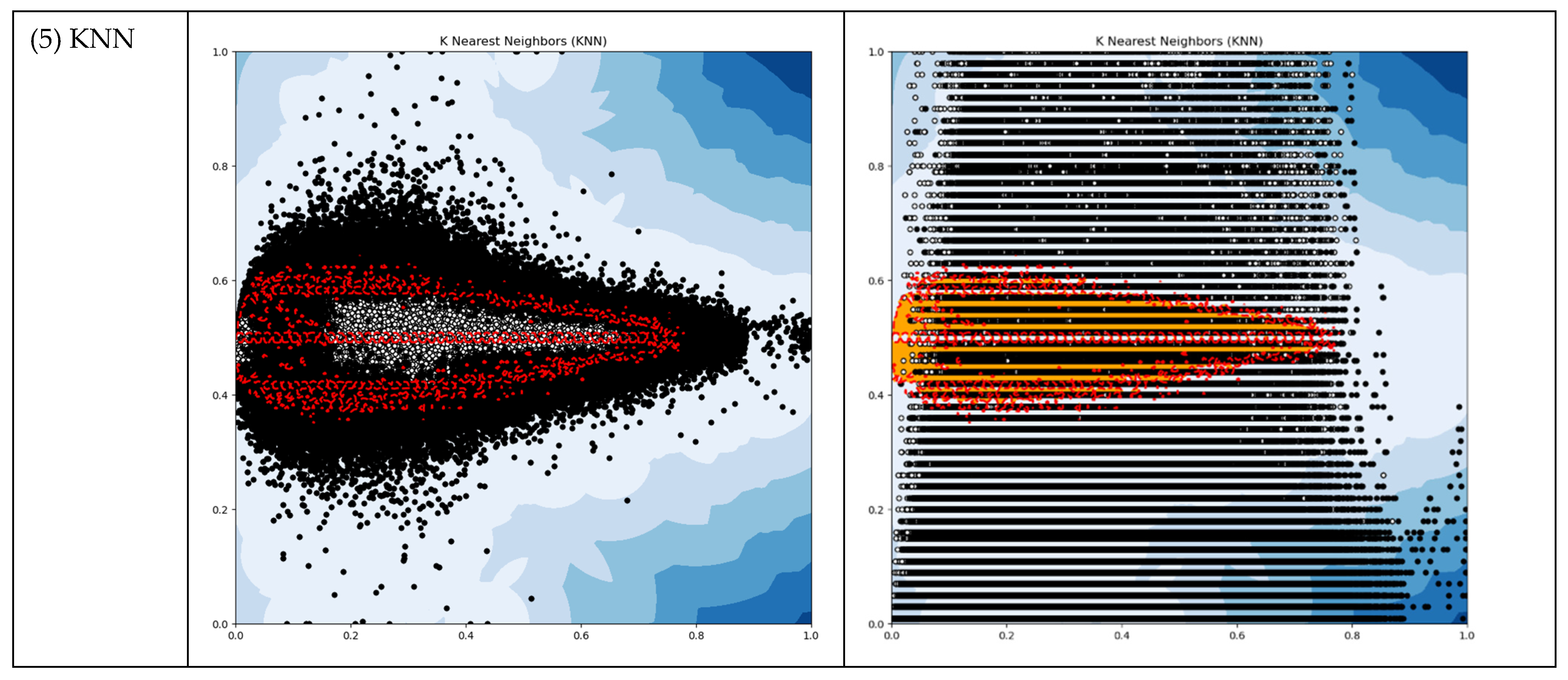
It would be convenient if we could leverage existing Outlier Detection (OD) algorithms. We conducted tests on our working data using typical unsupervised OD algorithms such as ABOD, CBLOF, HBOS, IF, and KNN. Our objective was to obtain thresholds from these OD algorithms that could subsequently be applied in the following modules. The results of these tests are presented in Table 2 and Figure 4.
Table 2.
Output of selected existing OD algorithms.
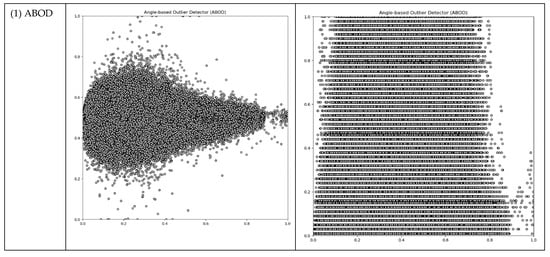
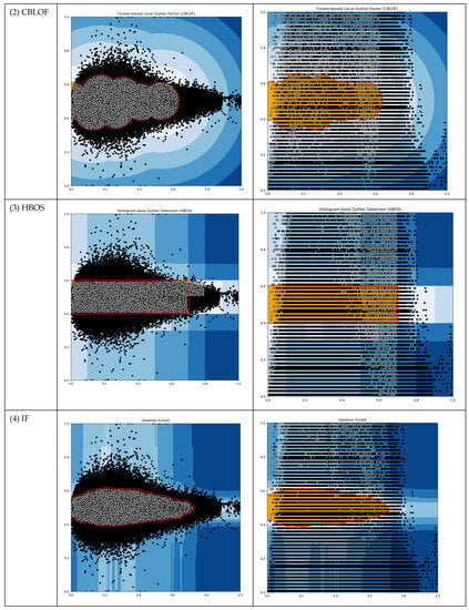
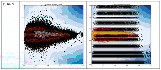
Figure 4.
The output plots of selected OD ML algorithms (Red dots represent threshold boundary; Black dots represent outliers).
The OD machine learning algorithms generated outlier counts, which amounted to approximately 5 percent of the total instances. This outcome was achieved by setting the “outlers_fraction” parameter to 0.05 during the testing process. However, for the subsequent modules of our DAD system, we required thresholds that possessed meaningful physical interpretations. Regrettably, none of these OD methods proved suitable for our DAD, as their threshold outputs did not align with our specific requirements.
In order to establish thresholds that were contextually relevant and aligned with the specific requirements of our Data Anomaly Detection (DAD) system, we first had to define “what is normal.” Previous research has indicated that driving patterns exhibit variations with changing speeds [33,51].
To address this, we organized the data into speed bins, each with a width of 1 mph, and grouped instances accordingly. For each speed bin, we computed the mean and standard deviations for each Key Performance Indicator (KPI). Consequently, we assembled a profile of what constitutes normal behavior for an individual vehicle. This profile is crucial information that needs to be extracted from historical BSMs, as detailed in Table 3.
Table 3.
Data panel extracted from BSMs of an individual vehicle (partial).
2.2.3. Module 3: Detecting Outliers
Outliers or anomalies are data points that do not conform to the conditions established for what is considered normal in Module 2. We assume that the BSMs follow a normal distribution, where data falling within the 95% probability region are categorized as normal, while the remaining 5% are designated as outliers. In statistical terms, the 95% cutoff value corresponds to the condition of being two times the standard deviation away from the mean.
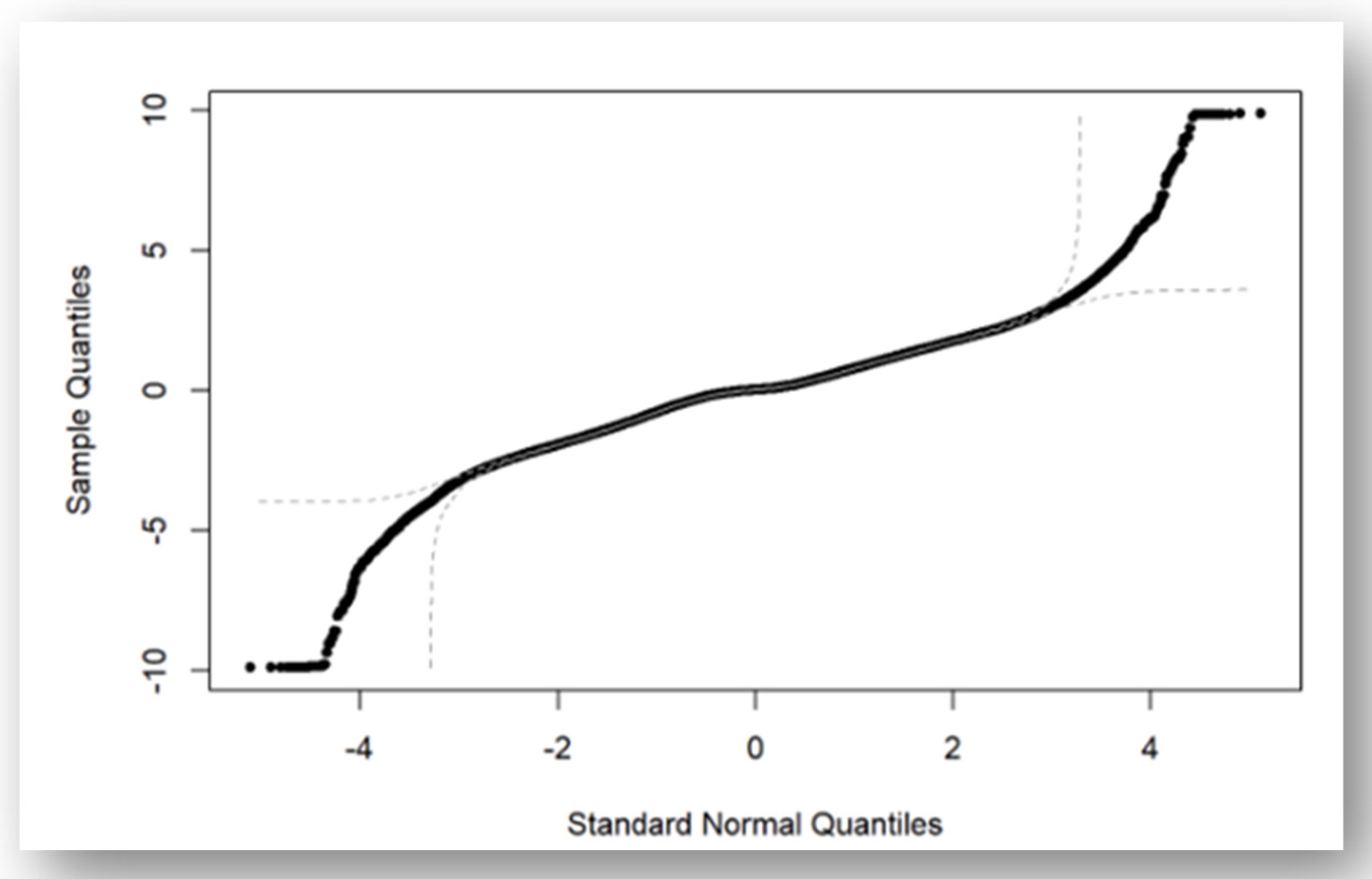
However, a valid question arises regarding our assumption: are the KPIs truly normally distributed? The answer is no, but there is a reasonably close approximation. For instance, when examining the longitudinal acceleration of ID 6010, it is evident that it does not strictly adhere to a normal distribution, but it does approximate one closely, as shown in Figure 5. The sample data roughly conforms to a normal distribution, but there are deviations at both extremes, which are guided with doted lines. Some researchers have suggested that it can be simulated using a Negative Binomial distribution [33]. Nevertheless, we have opted for an approximation of the normal distribution because we are addressing an engineering problem. Our primary concern is whether a vehicle has the potential to cause a crash, and we can rely on engineering solutions to address complex mathematical challenges. This philosophy aligns with our approach of handling the impact of coordinates (environmental factors) by deferring them to the CIM component.
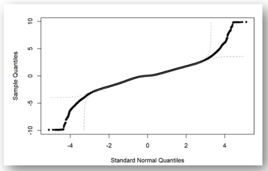
Figure 5.
Q-Q plot of longitudinal acceleration of a sample vehicle.
2.2.4. Module 4: Determine Abnormal Driving Event
In our assessments of Module 3, we observed the detection of numerous outliers, ranging from a few to thousands, depending on the driver and the duration of a trip file. This raised concerns about the potential for frequent alarms, which could irritate a driver. While a single outlier might not necessarily indicate abnormal driving status, the presence of multiple outliers occurring within a short time frame indeed signifies an anomaly. Consequently, we introduced Module 4 into our DAD model to mitigate the occurrence of false alarms. Given the absence of a labeled dataset, we turned to sensitivity analysis (SA) to fine-tune the model parameters. SA is a commonly used tool in model development that aids the determination of appropriate parameter values by observing how a dynamic model responds to various parameter settings. For the SA process, we established the following criteria: An abnormal event, capable of triggering an alarm for a abnormal driving event will be deemed valid if any of the following conditions are met:
- (1)
- The number of KPIs identified as outliers in the same second is larger or equal to Nv.
- (2)
- Within Ns, more than one KPI is identified as an outlier in a row,
where
- Nv—the number of KPIs identified as outliers in the same second;
- Ns—the number of successive seconds.
As we are interested in how the model would respond to how to define the in liners and how many days of historical BSMs need to be kept, the and were also included as a testing parameter, where:
- Nstd—the number of times of standard deviation away from the mean to calculate the thresholds;
- Nd—the number of days prior to the crash to calculate the threshold.
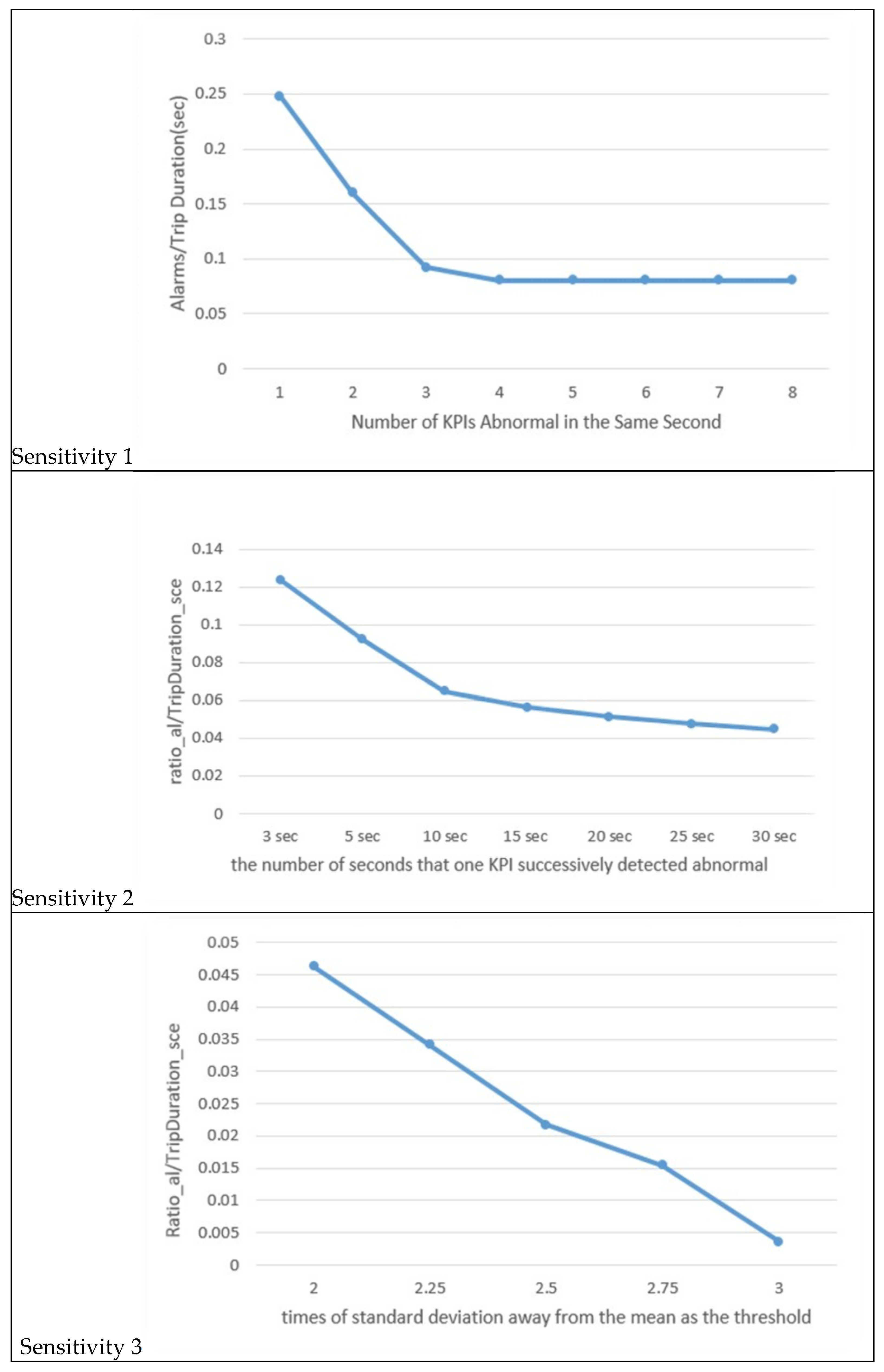
In our model, we work with a total of 8 Key Performance Indicators (KPIs), namely, acceleration—longitudinal, acceleration—lateral, jerk—longitudinal, and jerk—lateral. Each of these KPIs has both positive and negative counterparts. Sensitivity 1 in Figure 6 illustrates how the system responds to a step increase in (the number of vehicle instances). When is set to 1 or 2, we can observe that more than 15% of the trip seconds’ instances are identified as alarms, resulting in an excessive number of alarms. This is not practical. Moreover, detailed data records indicate that in many cases, both acceleration and jerk in the same direction are identified as outliers simultaneously, suggesting a degree of correlation between these pairs. Consequently, we ruled out values 1 and 2. When exceeds 3, the curve becomes relatively flat, signifying that the number of identified abnormal cases is very similar. Therefore, we settled on being equal to 3.
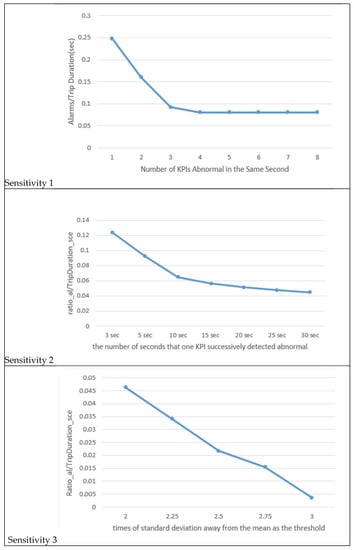
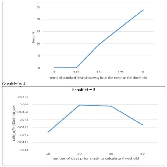
Figure 6.
Sensitivity analysis.
Sensitivity 2 in Figure 6 demonstrates the system’s response to a step increase in (the duration of the trip in seconds). We selected a value of 10 s for because this is where the curve exhibits a noticeable change in slope and the ratio value approaches 5%.
Sensitivity 3 in Figure 6 reveals the system’s response to a step increase in (the standard deviation multiplier). Notably, the values of 2 and 2.5 do not induce significant changes in the system’s response.
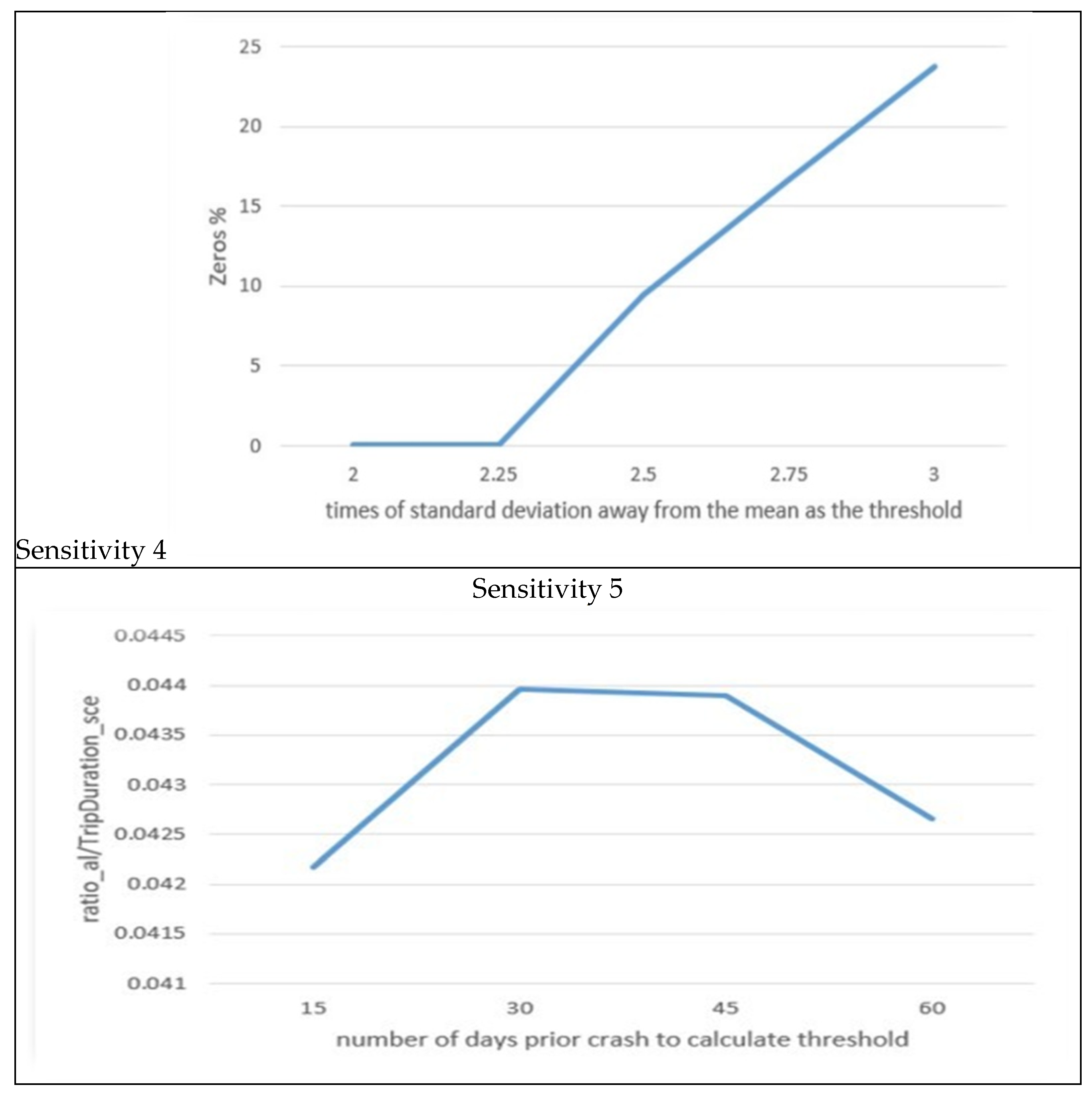
Moreover, Sensitivity 4 in Figure 6 indicates that after the value of 2.25, no alarms (Zeros %) are generated for the testing file. This contradicts the purpose of the model, which is to detect abnormalities related to potential crashes. Consequently, we opted for a value of 2 for as it is widely used and the difference between 2 and 2.25 is not substantial.
Sensitivity 5 in Figure 6 showcases the system’s response to a step increase in (the number of days for calculating thresholds). We assumed that the DAD employs batch mode for threshold calculation. The curve exhibits variations within a narrow range, indicating that the system is not highly sensitive to changes in We chose 30 days because this period allows for the identification of the most anomaly events. In practice, determining this parameter is more appropriate for considering the number of vehicles covered by a cloud and a server’s computational capacity. Additionally, it is important to note that auto-tuning is expected to replace the batch mode in the future, rendering this parameter obsolete. The results of the sensitivity analysis are summarized in Table 4.
Table 4.
Parameter settings for sensitivity analysis.
2.2.5. Module 5: System Updating
As previously mentioned, the system operates in an adaptive manner. Periodically, the system will perform a batch mode update for all the thresholds. The specific cycling time for these updates needs to be determined based on local conditions. Once the BSMs for the next cycle have been collected, the procedures outlined earlier will be repeated, and the thresholds will undergo an update accordingly.
3. Model Evaluation
Our DAD system was built on the assumption that when a CV is in an abnormal state, its trajectory will manifest a higher number of outliers compared to when it is in a normal state. We established the outlier factor at 95%, indicating that in normal driving conditions, outliers would constitute up to 5% of the data. To operationalize this, we derived the threshold criteria for what is considered normal from the historical BSMs of a specific CV and then applied these thresholds to real-time BSMs from the same CV.
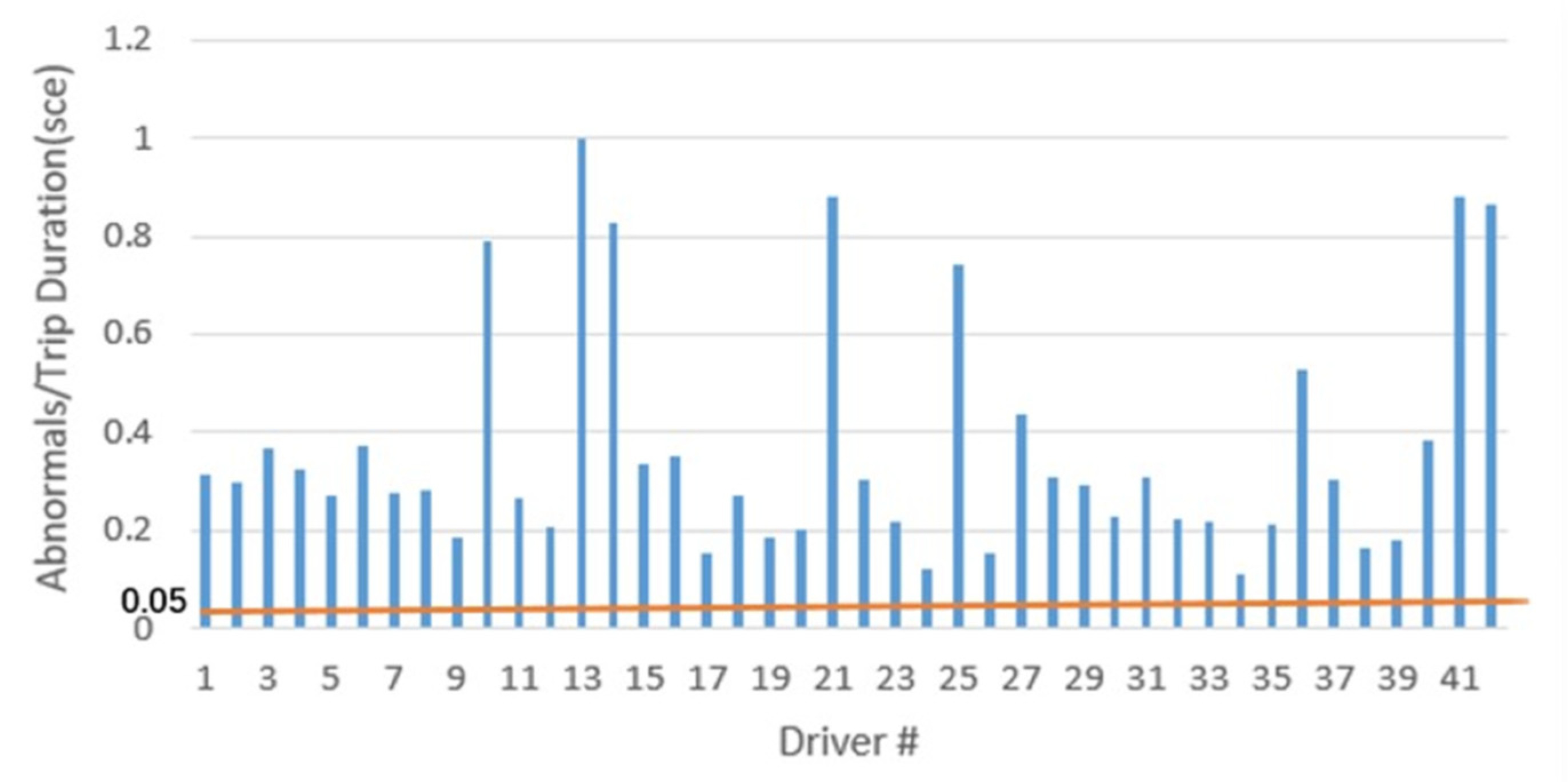
To verify the validity of the DAD system, we designed the following test: We selected 42 accident trip files from the SHRP2 data and tested them using the thresholds calculated based on each individual’s historical trajectories. If the number of detected anomaly cases exceeded 5%, the DAD model would be validated. The test results revealed that all 42 drivers exhibited more than 5% abnormal instances during the accident trips. This outcome provides strong evidence of the DAD model’s validity, as illustrated in Figure 7.
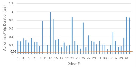
Figure 7.
Evaluation of the DAD model.
4. Discussion
Our development of the DAD system followed a series of standard TS analysis approaches, none of which revealed any discernible periodic patterns. This outcome was not surprising given the complexity of driving behavior, as most TS data in this context typically lack periodicity. Furthermore, our attempts to employ existing OD algorithms proved fruitless, as none of them were suitable for our specific requirements.
In response to these challenges, we embarked on creating the DAD system from the ground up, drawing upon insights from previous research. Our first significant contribution was the definition of a near-crash scenario, which we characterized as when at least one of the vehicles involved is in an abnormal driving state and a conflict is imminent.
While we assumed that the KPIs followed a normal distribution, it is worth noting that, strictly speaking, they do not adhere to this distribution. However, we considered this a reasonable relaxation because our primary objective was to determine whether the KPI values fell within the abnormal range. Once an anomaly was identified, our focus was on capturing it rather than predicting it using complex mathematical models. Another objective of this study was to explore methods for the reuse of BSMs. Traditionally, BSMs have been regarded as disposable data. However, with the widespread deployment of CVs, the sheer volume of BSMs generated can become overwhelming, making it impractical to store them all despite their valuable information. Nonetheless, it is feasible to extract and retain valuable information from BSMs. In line with this, we suggest utilizing the threshold criteria established for what is considered normal for an individual CV, which were derived as a result of Module 2 in the DAD system.
There are several limitations that provide avenues for future improvement in this study. Firstly, human behavior is intricate, and attempting to determine behavior status solely based on a vehicle’s footprint can pose a substantial challenge. In future research, it is imperative to involve cognitive science to enhance the robustness of the model. Secondly, although we conducted ANOVA tests and did not identify any statistical correlations among the KPIs, it is worth exploring further the potential correlations that might exist among these KPIs. Lastly, auto-tuning should have been implemented in Module 5 of our DAD; however, we opted not to employ auto-tuning in this context primarily due to constraints related to data availability. It is worth noting that detecting changes in driving habits often necessitates a more extended observation period than the one-month duration we had at our disposal.
5. Conclusions
In this paper, we share our experience in developing a Data Anomaly Detection (DAD) model designed to assess a driver’s abnormal driving status at the individual level, relying solely on Basic Safety Message (BSM) data. This represents a shift from the traditional method of highway patrol officers visually inspecting vehicle trajectories to identify traffic violations to a more automated approach where in-vehicle computers utilize computational models to flag driving anomalies. Given the complexity of human driving behavior, analyzing vehicle footprints can serve as an effective shortcut in this endeavor.
The main contribution of this paper lies in its pioneering approach to identifying near-crash scenarios on two specific conditions: Driving Anomalies (DAs) and conflicts. The paper establishes a system for scrutinizing driving anomalies at the individual level and demonstrates an effective methodology for handling intricate data such as BSMs. Instead of embarking on the development of intricate models to manage every attribute within a dataset, our approach involves the categorization of data attributes into two distinct groups: time-related and space-related. Subsequently, these attribute categories are addressed at separate stages, utilizing dedicated models, namely, the DAD and conflict identification model (CIM) modules.
It is worth emphasizing that our DAD system represents a preliminary exploration and merely scratches the surface of its potential. Creating a comprehensive DAD system of this nature could conceivably demand several years of work conducted by a team of data engineers to achieve full realization. We anticipate that our research will generate a systematic impact by reducing false traffic safety alarms, subsequently leading to a decrease in the occurrence of crashes and their associated effects on traffic congestion. Through this paper, our objective is to attract the attention of scholars and transportation professionals to the potential of DAD using the analysis of BSMs within the Connected Vehicle (CV) environment.
Author Contributions
Conceptualization, D.W., S.Z.T. and L.Z.; methodology, D.W., S.Z.T. and L.Z.; software, D.W.; validation, D.W.; formal analysis, D.W. and S.Z.T.; investigation, D.W. and S.Z.T.; resources, S.Z.T. and R.W.W.; data curation, D.W. and S.Z.T.; writing-original draft preparation, D.W.; writing-review and editing, S.Z.T.; visualization, D.W.; supervision, S.Z.T. and R.W.W.; project administration, S.Z.T. and R.W.W.; funding acquisition, S.Z.T. and R.W.W. All authors have read and agreed to the published version of the manuscript.
Funding
This research was funded by the U.S. Department of Transportation through the University of Florida Southeastern Transportation, Research, Innovation, Development, and Education (STRIDE) center under federal award number 69A3551747104.
Data Availability Statement
Data supporting reported results will be uploaded to the Zenodo repository at https://zenodo.org/deposit/new?c=stride-utc (accessed on 15 September 2022).
Conflicts of Interest
The authors declare no conflict of interest.
References
- Ahangari, S.; Jeihani, M.; Dehzangi, A. A machine learning distracted driving prediction model. In Proceedings of the 3rd International Conference on Vision, Image and Signal Processing, Vancouver, BC, Canada, 26–28 August 2019; pp. 1–6. [Google Scholar]
- Ahangari, S.; Jeihani, M.; Rahman, M.M.; Dehzangi, A. Prediction driving distraction patterns in different road classes using a support vector machine. Int. J. Traffic Transp. Eng. 2021, 11, 102–114. [Google Scholar]
- Ayuso, M.; Guillen, M.; Nielsen, J.P. Improving automobile insurance ratemaking using telematics: Incorporating mileage and driver behaviour data. Transportation 2019, 46, 735–752. [Google Scholar] [CrossRef]
- Banerjee, S.; Khadem, N.K.; Kabir, M.; Jeihani, M. Driver behavior post-cannabis consumption—A driving simulator study in collaboration with Montgomery County, Maryland. In Proceedings of the International Conference on Transportation and Development 2023, Austin, TX, USA, 14–17 June 2023; pp. 62–78. [Google Scholar] [CrossRef]
- Boukerche, A.; Zheng, L.; Alfandi, O. Outlier detection: Methods, models, and classification. ACM Comput. Surv. 2020, 53, 1–37. [Google Scholar] [CrossRef]
- Boyle, J.M.; Lampkin, C.; Schulman, R. Motor Vehicle Occupant Safety Survey. Volume 2, Seat Belt Report; No. DOT-HS-810-975; US Department of Transportation: Washington, DC, USA, 2007.
- Chandola, V.; Banerjee, A.; Kumar, V. Anomaly Detection: A Survey; ACM Computing Surveys (CSUR): New York, NY, USA, 2009; Volume 41, pp. 1–58. [Google Scholar]
- De Vlieger, I.; De Keukeleere, D.; Kretzschmar, J.G. Environmental effects of driving behaviour and congestion related to passenger cars. Atmos. Environ. 2000, 34, 4649–4655. [Google Scholar] [CrossRef]
- Di Cairano, S.; Bernardini, D.; Bemporad, A.; Kolmanovsky, I.V. Stochastic MPC with learning for driver-predictive vehicle control and its application to HEV energy management. IEEE Trans. Control Syst. Technol. 2013, 22, 1018–1031. [Google Scholar] [CrossRef]
- Dingus, T.A.; Guo, F.; Lee, S.; Antin, J.F.; Perez, M.; Buchanan-King, M.; Hankey, J. Driver crash risk factors and prevalence evaluation using naturalistic driving data. Proc. Natl. Acad. Sci. USA 2016, 113, 2636–2641. [Google Scholar] [CrossRef] [PubMed]
- Duan, L.; Xu, L.; Liu, Y.; Lee, J. Cluster-based outlier detection. Ann. Oper. Res. 2009, 168, 151–168. [Google Scholar] [CrossRef]
- Ellison, A.B.; Greaves, S. Driver characteristics and speeding behaviour. In Proceedings of the 33rd Australasian Transport Research Forum (ATRF’10), Canberra, Australia, 29 September–1 October 2010. [Google Scholar]
- Ericsson, E. Variability in urban driving patterns. Transp. Res. Part D Transp. Environ. 2000, 5, 337–354. [Google Scholar] [CrossRef]
- Fancher, P. Intelligent Cruise Control Field Operational Test; Final report. Volume II: Appendices A-F, Research report for National Highway Traffic Safety Administration; US Department of Transportation: Washington, DC, USA, 1998.
- Burnham, G.; Seo, J.; Bekey, G. Identification of human driver models in car following. IEEE Trans. Autom. Control 1974, 19, 911–915. [Google Scholar] [CrossRef]
- Goldstein, M.; Dengel, A. Histogram-based outlier score (hbos): A fast unsupervised anomaly detection algorithm. In KI-2012: Poster and Demo Track, Proceedings of the 35th German Conference on Artificial Intelligence, Saarbrücken, Germany, 24–27 September 2012; Springer Berlin: Heidelberg, Germany, 2012; Volume 1, pp. 59–63. [Google Scholar]
- Halim, Z.; Rehan, M. On identification of driving-induced stress using electroencephalogram signals: A framework based on wearable safety-critical scheme and machine learning. Inf. Fusion 2020, 53, 66–79. [Google Scholar] [CrossRef]
- Henclewood, D.; Abramovich, M.; Yelchuru, B. Safety pilot model deployment–one day sample data environment data handbook. In Research and Technology Innovation Administration. Research and Technology Innovation Administration; US Department of Transportation: McLean, VA, USA, 2014. [Google Scholar]
- Igarashi, K.; Miyajima, C.; Itou, K.; Takeda, K.; Itakura, F.; Abut, H. Biometric identification using driving behavioral signals. In Proceedings of the 2004 IEEE International Conference on Multimedia and Expo (ICME) (IEEE Cat. No.04TH8763), Taipei, Taiwan, 27–30 June 2004; Volume 1, pp. 65–68. [Google Scholar] [CrossRef]
- Jafari, M. Traffic Safety Measures Using Multiple Streams Real Time Data; Federal Highway Administration: Washington, DC, USA, 2017.
- Janai, J.; Güney, F.; Behl, A.; Geiger, A. Computer vision for autonomous vehicles: Problems, datasets and state of the art. arXiv 2017, arXiv:1704.05519. [Google Scholar]
- Kim, E.; Choi, E. Estimates of Critical Values of Aggressive Acceleration from a Viewpoint of Fuel Consumption and Emissions. In Proceedings of the Transportation Research Board 92nd Annual Meeting, Washington, DC, USA, 13–17 January 2013. [Google Scholar]
- Kriegel, H.P.; Schubert, M.; Zimek, A. Angle-based outlier detection in high-dimensional data. In Proceedings of the 14th ACM SIGKDD International Conference on Knowledge Discovery and Data Mining, Las Vegas, NV, USA, 24–27 August 2008; pp. 444–452. [Google Scholar]
- Lajunen, T.; Karola, J.; Summala, H. Speed and acceleration as measures of driving style in young male drivers. Perceptual and motor skills. Percept. Mot. Ski. 1997, 85, 3–16. [Google Scholar] [CrossRef]
- Langari, R.; Won, J.-S. Intelligent energy management agent for a parallel hybrid vehicle-part I: System architecture and design of the driving situation identification process. IEEE Trans. Veh. Technol. 2005, 54, 925–934. [Google Scholar] [CrossRef]
- Larose, D.T.; Larose, C.D. k-nearest neighbor algorithm. In Discovering Knowledge in Data: An Introduction to Data Mining; Wiley: Oxford, UK, 2014; pp. 149–164. ISBN 9780470908747/0470908742. [Google Scholar]
- Lees, M.N.; Cosman, J.D.; Lee, J.D.; Fricke, N.; Rizzo, M. Translating cognitive neuroscience to the driver’s operational environment: A neuroergonomic approach. Am. J. Psychol. 2010, 123, 391–411. [Google Scholar] [CrossRef] [PubMed]
- Liang, Y.; Lee, J.D. Combining cognitive and visual distraction: Less than the sum of its parts. Accid. Anal. Prev. 2010, 42, 881–890. [Google Scholar] [CrossRef] [PubMed]
- Liaw, B.Y.; Bethune, K.P.; Kim, C.S. Time-series field trip data analysis using adaptive recognition approach. Analysis on driving patterns and vehicle usage for electric vehicles. In Proceedings of the 19th Electric Vehicle Symposium (EVS-19), Busan, Republic of Korea, 19–23 October 2002; pp. 19–23. [Google Scholar]
- Li, L.; You, S.; Yang, C.; Yan, B.; Song, J.; Chen, Z. Driving-behavior-aware stochastic model predictive control for plug-in hybrid electric buses. Appl. Energy 2016, 162, 868–879. [Google Scholar] [CrossRef]
- Liu, J.; Khattak, A.J. Delivering improved alerts, warnings, and control assistance using basic safety messages transmitted between connected vehicles. Transp. Res. Part C Emerg. Technol. 2016, 68, 83–100. [Google Scholar] [CrossRef]
- Liu, J.; Wang, X.; Khattak, A.J. Generating real-time driving volatility information. In Proceedings of the 2014 World Congress on Intelligent Transport Systems, Detroit, MI, USA, 11 September 2014. [Google Scholar] [CrossRef]
- Martinez, C.M.; Heucke, M.; Wang, F.-Y.; Gao, B.; Cao, D. Driving style recognition for intelligent vehicle control and advanced driver assistance: A survey. IEEE Trans. Intell. Transp. Syst. 2017, 19, 666–676. [Google Scholar] [CrossRef]
- Miyaji, M.; Danno, M.; Oguri, K. Analysis of driver behavior based on traffic incidents for driver monitor systems. In Proceedings of the 2008 IEEE Intelligent Vehicles Symposium, Eindhoven, The Netherlands, 4–6 June 2008; pp. 930–935. [Google Scholar] [CrossRef]
- Tselentis, D.I.; Papadimitriou, E. Driver profile and driving pattern recognition for road safety assessment: Main challenges and future directions. IEEE Open J. Intell. Transp. Syst. 2023, 4, 83–100. [Google Scholar] [CrossRef]
- Murphey, Y.L.; Milton, R.; Kiliaris, L. Driver’s style classification using jerk analysis. In Proceedings of the 2009 IEEE Workshop on Computational Intelligence in Vehicles and Vehicular Systems, Nashville, TN, USA, 30 March–2 April 2009; pp. 23–28. [Google Scholar]
- Prokop, G. Modeling human vehicle driving by model predictive online optimization. Veh. Syst. Dyn. 2001, 35, 19–53. [Google Scholar] [CrossRef]
- Reason, J. Human Error; Cambridge University Press: Cambridge, UK, 1990. [Google Scholar]
- Venkatraman, V.; Richard, C.M.; Magee, K.; Johnson, K. Countermeasures That Work: A Highway Safety Countermeasure Guide for State Highway Safety Offices; National Highway Traffic Safety Administration: Washington, DC, USA, 2017.
- Sekizawa, S.; Inagaki, S.; Suzuki, T.; Hayakawa, S.; Tsuchida, N.; Tsuda, T.; Fujinami, H. Modeling and recognition of driving behavior based on stochastic switched ARX model. IEEE Trans. Intell. Transp. Syst. 2007, 8, 593–606. [Google Scholar] [CrossRef]
- Sun, X.; Cao, Y.; Jin, Z.; Tian, X.; Xue, M. An adaptive ECMS based on traffic information for plug-in hybrid electric buses. IEEE Trans. Ind. Electron. 2022, 70, 9248–9259. [Google Scholar] [CrossRef]
- Sun, X.; Xue, M.; Cai, Y.; Tian, X.; Jin, Z.; Chen, L. Adaptive ECMS Based on EF Optimization by Model Predictive Control for Plug-In Hybrid Electric Buses. IEEE Trans. Transp. Electrif. 2022, 9, 2153–2163. [Google Scholar] [CrossRef]
- Victor, T.; Dozza, M.; Bärgman, J.; Boda, C.N.; Engström, J.; Flannagan, C.; Lee, J.D.; Markkula, G. Analysis of Naturalistic Driving Study Data: Safer Glances, Driver Inattention, and Crash Risk; Transportation Research Board: Washington, DC, USA, 2015. [Google Scholar]
- Wang, X.; Khattak, A.J.; Liu, J.; Masghati-Amoli, G.; Son, S. What is the level of volatility in instantaneous driving decisions? Transp. Res. Part C Emerg. Technol. 2015, 58, 413–427. [Google Scholar] [CrossRef]
- William, H.J. Advances in the Epidemiology of Injures as a Baiss for Public Policy. Public Hearlth Rep. 1980, 95, 411. [Google Scholar]
- Wilson, F.N.; Johnston, F.D.; Macleod, A.; Barker, P.S. Electrocardiograms that represent the potential variations of a single electrode. Am. Heart J. 1934, 9, 447–458. [Google Scholar] [CrossRef]
- Wu, D.; Zhang, L.; Whalin, R.; Tu, S. Conflict Identification Using Speed Distance Profile on Basic Safety Messages. In Proceedings of the International Conference on Transportation and Development, Seattle, WA, USA, 31 May–3 June 2022. [Google Scholar]
- Xu, D.; Wang, Y.; Meng, Y.; Zhang, Z. An Improved Data Anomaly Detection Method Based on Isolation Forest. In Proceedings of the 10th international symposium on computational intelligence and design (ISCID), Hangzhou, China, 9–10 December 2017; IEEE: Piscataway, NJ, USA; Volume 2, pp. 287–291. [Google Scholar] [CrossRef]
- Yang, X.; Zou, Y.; Chen, L. Operation analysis of freeway mixed traffic flow based on catch-up coordination platoon. Accid. Anal. Prev. 2022, 175, 106780. [Google Scholar] [CrossRef]
- Zamith, M.; Leal-Toledo, R.C.P.; Clua, E.; Toledo, E.M.; de Magalhães, G.V. A new stochastic cellular automata model for traffic flow simulation with drivers’ behavior prediction. J. Comput. Sci. 2015, 9, 51–56. [Google Scholar] [CrossRef]
- Zhao, Y.; Nasrullah, Z.; Li, Z. Pyod: A python toolbox for scalable outlier detection. arXiv 2019, arXiv:1901.01588. [Google Scholar]


Disclaimer/Publisher’s Note: The statements, opinions and data contained in all publications are solely those of the individual author(s) and contributor(s) and not of MDPI and/or the editor(s). MDPI and/or the editor(s) disclaim responsibility for any injury to people or property resulting from any ideas, methods, instructions or products referred to in the content. |
© 2023 by the authors. Licensee MDPI, Basel, Switzerland. This article is an open access article distributed under the terms and conditions of the Creative Commons Attribution (CC BY) license (https://creativecommons.org/licenses/by/4.0/).