1. Introduction
Nowadays, the automotive industry is trying to reduce costs and replace more and more physical sensors with virtual sensors. Therefore, a feasibility study was carried out within the framework of a master’s thesis to understand whether it is possible to predict a passenger car wheel torque signal with the help of a neural network, and whether it is possible to transfer the model structure from a torque prediction to a temperature prediction. Vehicle signals were stored as time series to describe the change of vehicle characteristics, such as speed, acceleration, etc., over time. Recurrent neural networks (RNNs) are normally used for timeseries prediction, which also include the previous timestep to predict the next one [
1]. A special form of an RNN is the long short-term memory (LSTM). LSTM has the advantage that it is not susceptible to the vanishing gradient problem, as observed with RNNs [
2].
Other studies have already addressed similar issues, for example trying to predict the mass of a vehicle using CAN data and a driveline torque observer [
3]. The vehicle data used in [
3] were recorded under laboratory conditions. In contrast, the data for this paper were generated without any specifications regarding driving style, route or distance. The difference between the two studies is in the quantity and quality of the data. Thus, the data in the study under laboratory conditions has more quality, whereas this study is set apart by the large mass of data. Further studies have, in addition to the prediction of vehicle masses using a neural network [
3], dealt with the prediction of engine torques and emission values [
4], or the engine torque and brake specific fuel consumption prediction, whereby a model was trained with only 81 datasets [
5]. Another paper dealt with the prediction of unsprung masses using a neural network, but using simulation data instead [
6]. One more study compared the prediction quality of Markov chains and recurrent neural networks [
7]. Here, the vehicle speed for the next time steps was predicted. Data from 36 trips on a specified
km route on public roads were used as input. Shin et al. [
7] used a fixed route on a public road, while in this study, no specific route with 1775 trips and 30,000 km from everyday life were chosen. In addition, the quantity of data differs between the two studies.
Some other studies also predicted different torque signals without using artificial intelligence. For example, an observer-based system in order to reconstruct the clutch torque and transmission output torque in [
8].
For this study, road load data were collected using a company car from the controller area network (CAN) bus (without measurement technique), and the data were used for a feasibility study to determine whether it is possible to train a neural network to predict a torque signal with real road load data that are not created under laboratory conditions. The vehicle was left in its standard condition and no non-standard components other than the data logger were installed. The mentioned company car was a Jaguar Land Rover
Evoque (model year 14, produced in 2017) with a
Twinster gearbox from
GKN Automotive. The Twinster enables the all-wheel drive to disconnect the rear-wheel drive from the front-wheel drive so only the front transfers torque to the road. This has multiple advantages for the driver, such as less fuel consumption, a good impact of the driving dynamics, and improved lateral and longitudinal vehicle dynamics [
9]. The disconnect function of the rear axle creates additional complexity in the torque signal by suspending the torque transmission. The opensource software
Python was selected to create the neural network, specifically
tensorflow. Tensorflow is an open-source framework for machine learning that is commonly used for building up neural networks.
The volume of the data allowed for a feasibility study to be conducted regarding a virtual sensor using a neural network. The target signal selected was the one that had the greatest influence on the driving behavior: the signal indicating how much torque is transferred by the rear axle. The Twinster gearbox two clutches that transfer the torque from the propshaft to each sideshaft. By applying an individual torque on each sideshaft, the vehicle receives better driving dynamics, as mentioned previously. The torque applied to the clutches was predicted in this study. The questions we sought to answer are as follows: Is it possible to predict the torque signal? How much data are needed to predict the torque signal? How good is the prediction accuracy?
In addition to the above-mentioned feasibility study, we investigated whether the model can be applied to a further problem. Because the clutch temperature of the Twinster gearbox is of great interest, the question arose as to whether the structure of the neural network for the torque signal could be transferred to a temperature signal. Therefore, another dataset from a prototype vehicle with additional non-standard measurement equipment was used for this case. The measurement equipment was used during the development phase to measure the clutch temperature. It was from the same type of vehicle but only a fraction of the trips were used for the torque signal: 36 trips for the temperature instead of 1775 trips for the torque prediction.
First, the data on which the work is based and the procedure for data preparation are discussed. In the next step, the model used for this work and its optimization are described. Then, the results are presented, discussed, and conclusions are drawn.
2. Materials and Methods
2.1. Data
A road load dataset covering 2 years, 1775 trips, and a total distance of 28,399.47 km was analyzed. These data were collected using the data logger µCROS 1.1 from IPETRONIK. The data logger records all of the vehicle data from the CAN bus (around 120 signals) and stores them into MF4 files with a frequency of 500 Hz. Those signals are mixed between actual signals and computed signals by the electronic control unit (ECU).
The vehicle data covered 2 years and 1775 trips. The data examined in this evaluation were collected primarily on public roads. No distinction was made between the different types of roads. The mean distance per trip was 16 km and the standard deviation was 30 km. This reflects the classic travel distance for everyday life: predominantly work trips and longer individual trips, which increase the standard deviation. Analogously, the mean trip duration was 20 min and its standard deviation was min. To be able to handle this amount of data, a special pre-process had to be developed. In this process, every file had to be normalized. Here, all signals were brought to the same sampling rate and all signal names were uniformly set for all files. With a view to reading and storing the performance of these vehicle data, the normalized data were stored as PARQUET files. The normalized PARQUET files allocate about 14 GB of hard disk (compared to approximately 200 GB of uncompressed MF4 files. For the whole data pre-processing, the Python libraries scikit-learn and pandas were used. Pandas is an open-source library that is created for data analysis. Scikit-learn can be used also for data analysis, but it also contains some easy algorithms for machine learning.
The first step was to check whether each measurement was suitable for the subsequent learning process. Upon selecting the valid trips that contained all of the required signals, 1661 files were left for creating the model.
In order to create a neural network, it is mandatory to split the data into training and testing datasets. A train–test split with 80% training data and 20% testing data was chosen (see
Figure 1). In the first step, the complete dataset was split into training and testing data at a ratio of 80/20. In a next step, the training data were split one more time into pure training data and validation data (same ratio). Validation data are needed for the algorithm to control the accuracy during training by itself [
10].
So, 1328 of the trips were used to train the neural network and 333 trips were reserved for testing the model performance and quality. The data were fitted to the model in multiple loops because the data were stored in multiple files and the files were too big for the random access memory (RAM). Additionally, the training and testing were split, the training dataset was split into training and validation data [
10]. Individual files were not split up for the train–test split. The validation took place during the training, so the last 20% of each trip was used for validation.
Upon splitting the data, the input parameters were defined. Out of the 120 signals per trip, the signals that had an influence on the torque signal were selected. The following signals from the data were used:
Side shaft speed (front left and right, rear left and right);
Longitudinal vehicle acceleration;
Latitudinal vehicle acceleration;
Longitudinal vehicle speed;
Throttle position;
Steering wheel angle;
Steering wheel angle speed;
Actual throttle position;
Actual engine torque;
Connect status of rear axis;
Electronic stability program (ESP) signal;
Anti-lock braking system (ABS) signal.
These signals were selected because they influence the torque signal and are also used by the ECU to generate the real torque signal. Signals, such as wiper status, rain sensor request, and vehicle voltage level, were not selected for input data, because they have no influence on the torque level. Additional input signals were generated through feature engineering [
11]. For example, this generated further input signals such as wheel slip for each wheel and the throttle change for each time step.
Categorical features, such as connect status, were also transformed into separate features using the Python pandas function get_dummies.
Analogously to the input features for the torque prediction, the input features for the temperature prediction were selected for their influence on the temperature:
Side shaft speed (front left and right, rear left and right);
Longitudinal vehicle acceleration;
Latitudinal vehicle acceleration;
Longitudinal vehicle speed;
Throttle position;
Steering wheel angle;
Steering wheel angle speed;
Actual throttle position;
Actual engine torque;
Connect status of rear axis;
ESP signal;
ABS signal;
Slip (front left and right, rear left and right);
Ambient temperature;
Established clutch torque;
Power (rear right and left).
Upon selecting all of the input features, the pre-processing was finished by scaling the data using MinMaxScaler (from scikit-learn).
2.2. Neural Network Design
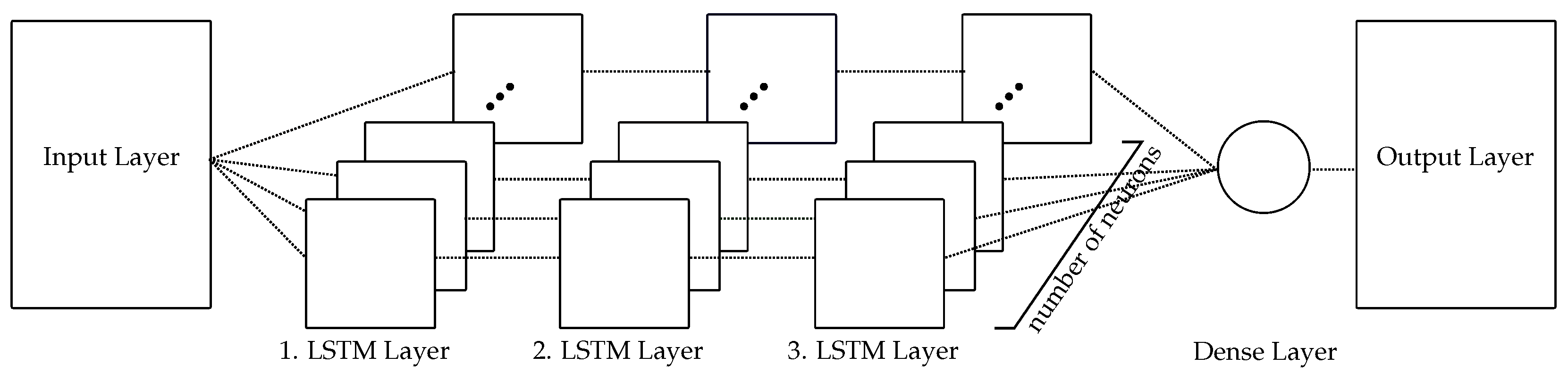
A time series signal should be predicted, so a recurrent neural network was selected for this problem. In [
12], a similar task used long short-term memory (LSTM) cells to predict the angle of the role. Because of the similarity, the structure of the model from [
12] was used here: three layers of LSTM cells followed by a forward directed dense layer with only one neuron were used to build the model, as can be seen in
Figure 2. The number of neurons for each LSTM layer was identified during the hyperparameter tuning in the next step.
The model was trained using a graphics processing unit (GPU), so there was no choice for different activation functions and the default
tanh function was used [
13]. With hyperparameter tuning, the best combination of fast runtime and best accuracy can be achieved. The following hyperparameters in
Table 1 were tested during tuning:
For the optimizer, the adam, adadelta, and rmsprop optimizers were tested. With respect to the number of neurons per LSTM layer, the numbers 150, 200, and 300 were compared. The batch sizes 128, 256, 512, and 1024 were tested as well as the number of inputs with 200, 400, and 800, which corresponded to 1, 2, and 4 s of data that were used to predict the next timestep.
The hyperparameter tuning was performed on a randomly assembled test dataset. The results of the hyperparameter tuning were compared by their , , and values. Scikit-learn contains a function called GridSearchCV that builds up a matrix of all combinations of hyperparameters that are given to the function, and runs the model and gives back the best combination of hyperparameters that is found. This function is not applicable in combination with tensorflow, so the workflow of this function was used and copied to a simple for loop.
The best ten results differed by around 9%, the best prediction matched the true signal by 57%. In addition to accuracy, training time also played a crucial role. The training time differed between 2 h (the slowest hyperparameter combination) and 47 min (the fastest combination). The decision for the best hyperparameter combination was set on a compromise between accuracy and training time. The decision was made for the fastest hyperparameter combination with 47 min and an accuracy of 50%:
Optimizer: adadelta;
Batch size: 1024;
Number of neurons (first layer): 200;
Number of neurons (second layer): 200;
Number of neurons (third layer): 150;
Number of inputs: 200.
3. Results
There were multiple results that needed to be evaluated and compared. With regard to identifying the impact of the size of the training dataset, the original training dataset was split into multiple sizes (10%, 20%, 50%, 80%, and 100%) so that, for example, only 10% of the trips were used to train the model. These results proved to improve the prediction accuracy.
Table 2 shows the numerical results of the trained models with different training dataset sizes. For each dataset, the coefficient of determination
, mean squared error (
), and the root mean squared error (
) were computed to show the performance of the models trained by the training datasets of different sizes. The table shows an increase in accuracy with more training data. An increasing accuracy becomes apparent with the increasing size of the training data. However, it can also be seen that the accuracy did not improve further after gaining an accuracy of 55% and an
value of
.
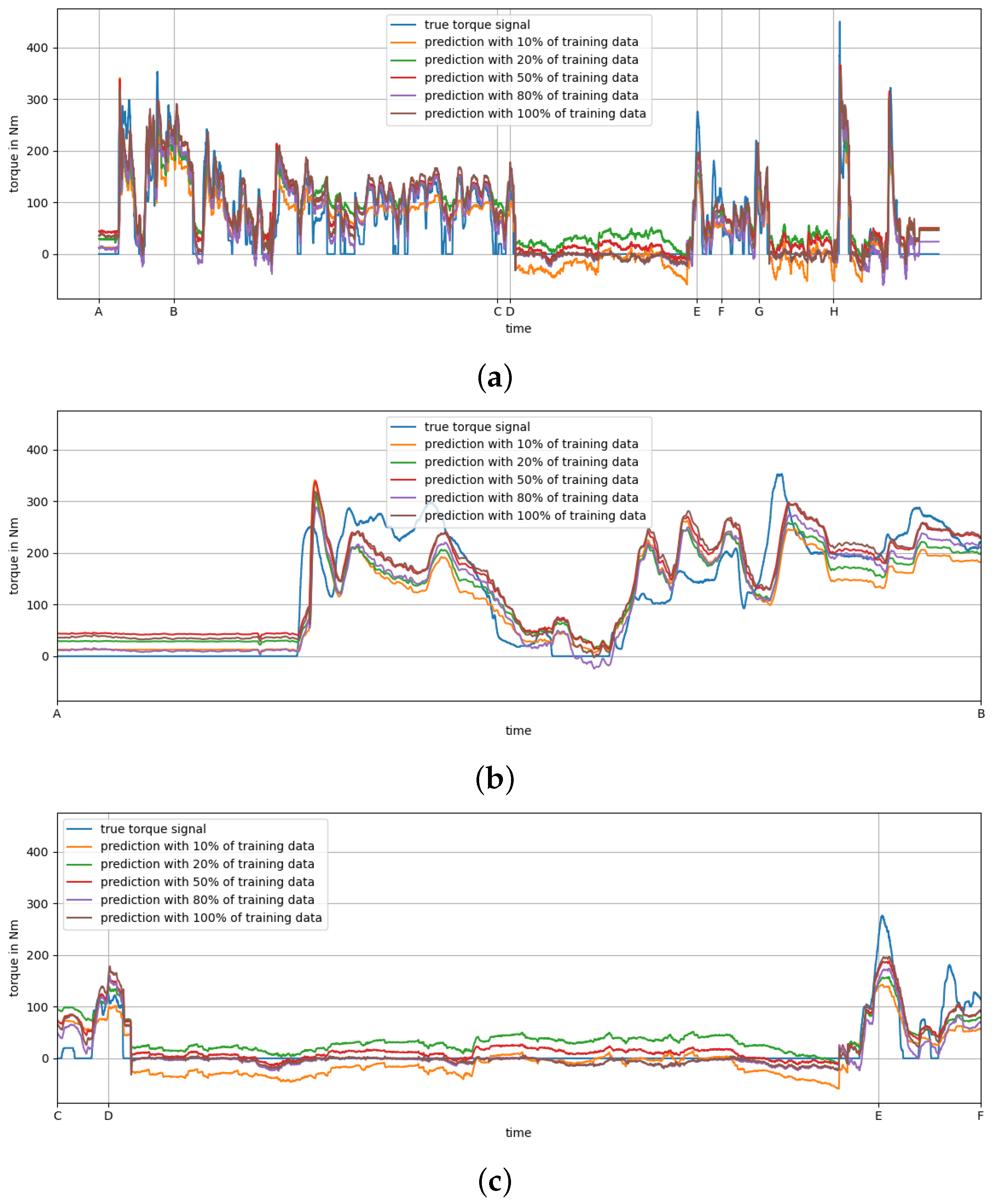
Figure 3 shows the graphic results of the prediction. Each prediction of every trained model from
Table 2 is plotted with the true torque signal. The true torque signal is in blue, the prediction of the model that was trained with 10% of the training data is in orange, for the model trained with 20%, the prediction is in green, for 50%, the prediction is in red, for 80%, the prediction is in violet, and the prediction that is based on all of the training data is in brown. This particular trip has an accuracy of 77.73%.
Figure 3a shows the entire test trip and its predictions.
Figure 3b shows the first part of the trip. It highlights the displacement of the signal while the rear axle does not transfer any torque.
Figure 3c shows another example for the displacement in the disconnect phase. Here, it can also be seen that the prediction improves as the training dataset increases in size.
The results show that it was possible to predict the given torque signal up to an accuracy of 55%. At the same time, it shows that some peaks were not well predicted by the neural network and that the prediction reacted rather slowly. Especially affected were the high peaks, e.g., at point
E and
H in
Figure 3a. These deflections could not be reproduced well by the neural network. The need for optimization was also seen for the time periods in which the rear-wheel drive was disconnected and 0
should have been transferred, see
Figure 3a,b. There, the prediction of the neural network had the biggest issues. The areas in which the rear axle was decoupled (
D to
E, see
Figure 3c, and
G to
H, see
Figure 3a), show strong noise (±50 Nm). In the first seconds of this run (see
Figure 3b) however, this strong noise did not occur. Here, the best prediction was slightly offset above the true signal by about 11
. Another aspect that was not correctly reproduced by the neural network was the fact that the real signal never became negative. Neither in the training data nor in the test data did the controller of the vehicle require a negative torque signal. Nevertheless, the neural network calculated a negative torque (see
Figure 3). However, this happened exclusively in the phases in which the all-wheel drive (AWD) was switched off.
In addition to investigating the feasibility of the prediction of the torque signal with a neural network, the transferability of the model to another signal was investigated. Therefore, another dataset was used, see
Section 1. The same pre-processing was executed, and the same model structure and hyperparameters that were used for the training of the torque signal were used here. Another difference was the train–test split ratio. Because there were only 36 trips available, 35 trips were used for training and only one for testing, instead of an 80/20 split, as stated in
Section 2.1.
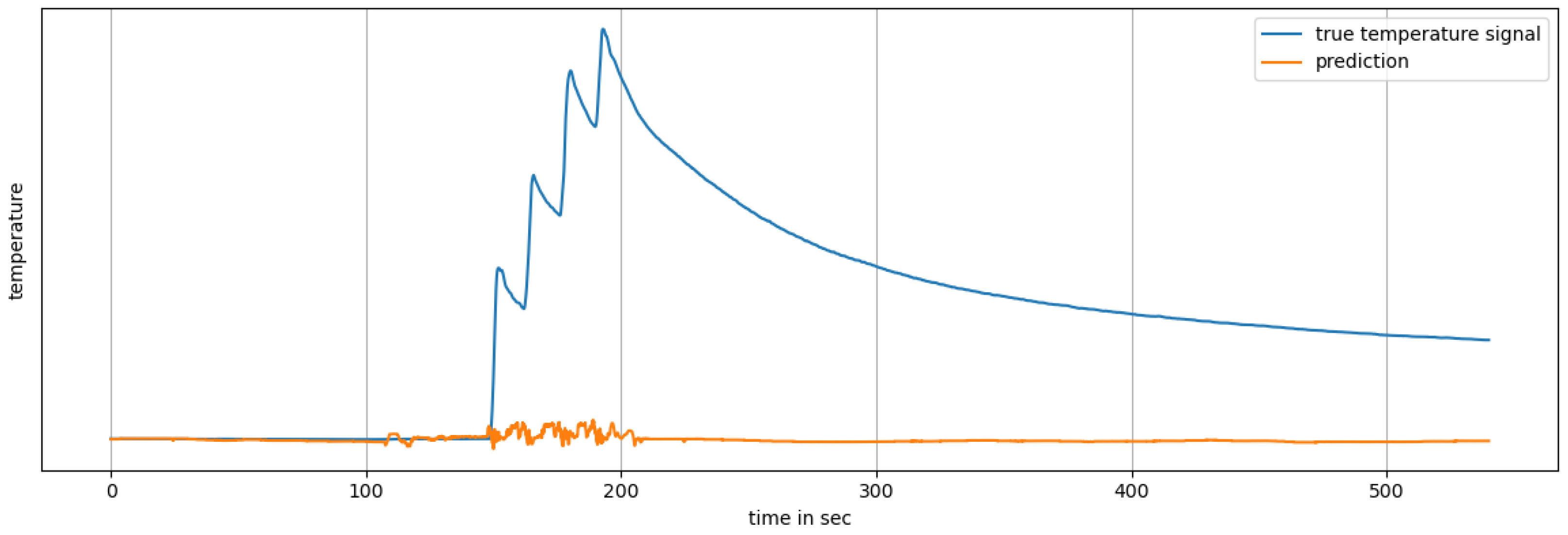
Figure 4 shows the graphical performance of the temperature prediction. It shows that the data do not match the true temperature signal at all. In particular, the step where the temperature increases very quickly is not reproduced by the neural network. It can be seen that it is not possible to predict the temperature in this initial simulation. In numbers, the prediction of the temperature signal scored an
of
°C and an
of −1.396.
4. Discussion
The results show that prediction with the help of a neural network is possible in principle. The conformity, as measured by the
value, could possibly be expanded by extending the hyperparameter tuning. Furthermore, the structure of the neural network was not further analysed in this work. As mentioned in
Section 2.2, the structure was taken from another case study that was similar to the case study described in this work.
There are multiple opportunities to further optimize the neural network, for example, by deeper and more extensive hyperparameter tuning and/or increasing the number of LSTM layers in the model structure.
One further try at optimization was carried out during the study by raising the number of epochs. Instead of 10 epochs per trip, the number of epochs was raised to 1000 in combination with the EarlyStopping function. The EarlyStopping function makes sure that if a given quality criterion does not improve after a defined number of epochs, the run is interrupted, and in this case the next training trip will start.
This procedure was tried on the 10% training dataset for keeping the run time as low as possible. The results of the new run were not better at all. With a new accuracy of only 43.86% and an
value of
, the new model was even slightly worse than the original 10% model (see
Section 2), and the calculation time increased by a factor of 15.
The transferability of the model of the torque signal to the temperature signal was unsuccessful. The reason for the failure was not analyzed further, but the likely assumption is that the small dataset caused the failure. On the one hand, this issue can be dealt with by changing the hyperparameters and changing the model structure of the neural network. On the other hand, if doing so does not show any effect, it is clear that the training data were much too small.
A few small improvement attempts were also tried during the transferability studies. For example, as with the torque prediction, the number of epochs was raised to improve the prediction accuracy in combination with the EarlyStopping function, and in another run, the loss function was changed from to mean squared log error ().
The results of these improvement attempts are displayed in
Table 3. The first line shows the results of the original model from
Table 2. The second line shows the results of the model with 500 epochs and
EarlyStopping. The last line of the table shows the results of the model with the
loss function. With a view to the
values, the results also show that in this case, the higher number of epochs did not have any impact on the results. The changing loss function had a small impact on the performance and improved the
from
to
(see
Table 3).
These new and unique results show that there is a difference between the prediction accuracy of neural networks that are trained with real road load data from every day use and those that are recorded under laboratory conditions in specific selected driving maneuvers [
3] or with simulated data [
6].
5. Conclusions
The feasibility studies determined that it is possible to predict a torque signal in general using a large amount of data that are not selected from a maneuver collection that is generated under laboratory conditions. It showed that a large training dataset is needed to improve the accuracy of the prediction. The best prediction achieved an accuracy of 55.85% with an of . With further improvement and optimization, the developed model could be used for a virtual sensor and replace physical sensors in the vehicle. This replacement saves on costs and weight for the automotive manufacturer.
The investigation into the transferability showed that under the given conditions, a transfer of the model structure from the torque signal to the temperature signal is not possible.
All in all, the investigation showed that it is possible to predict a torque signal with a good accuracy and the results can be used to conduct further research with respect to a virtual sensor. Other fields of application could be the use of a torque or temperature neural network model for digital twins during the advancement of the system, or in automation.


