Abstract
The topics of climate change and pollutant emission reduction are dominating societal discussions in many areas. In automotive development, with the introduction of real driving emissions (RDE) testing and the upcoming EU7 legislation, there are endless boundary conditions and potential scenarios that need to be evaluated. In terms of vehicle calibration, this is leading to a strong focus on alternative approaches such as virtual calibration. Due to the flexibility of virtual test environments and the variety of RDE scenarios, the amount of data collected is rapidly increasing. Supporting the calibration engineers in using the available data and identifying relevant information and test scenarios requires efficient approaches to data analysis. This paper therefore discusses the potential of data clustering to support this process. Using a previously developed approach for event detection in emission calibration, a methodology for the automatic categorization of events is presented. Approaches to clustering algorithms (hierarchical, partitioning, and density-based) are discussed and applied to data of interest. Their suitability for different signals is investigated exemplarily, and the relevant inputs are analyzed for their usability in calibration procedures. It is shown which clustering approaches have the potential to be implemented in the vehicle calibration process to provide added value to data evaluation by calibration engineers.
1. Introduction
The constant need to optimize modern passenger cars in terms of sustainability, price, emission reduction [1,2], and quality places high demands on the development processes [3,4,5]. Constantly updated and intensified emission standards, such as the Euro 6d introduced in 2017 [6,7] or the upcoming Euro 7 regulations [8], set new framework conditions specifically for the series calibration process of modern vehicles [9,10,11]. To ensure legal compliance under all relevant conditions and to increase the efficiency in daily use, topics such as base calibration, drivability calibration, emission calibration, or operating strategy calibration are using new approaches in their daily processes in order to achieve zero-impact emission vehicles [2,12,13,14].
Innovative approaches aim to reduce costs, shorten the time to market, and reduce the number of prototype vehicles while maintaining or even increasing quality levels. A central topic in this context is the virtualization and simulation of development tasks. Conventional processes are partly replaced and supplemented by simulation-based enhancements [15]. The use of simulation-based approaches allows the speed of test execution and data acquisition to increase. Initial boundary conditions and changes to setups can be adapted more quickly and soaking phases, for example, can be shortened. However, the resulting potential in data acquisition can only be effectively exploited if the data analysis procedures are adapted at the same time.
In the field of vehicle series calibration, this represents a major challenge. In the conventional process, each discipline of series calibration (such as baseline, emissions, drivability, hybrid operating strategy, or OBD calibration) currently performs its own tests, including data acquisition and analysis. The data are usually analyzed manually. For example, each emission test performed is examined by a calibration engineer. Due to lack of time, usually only tests that show exceptional cumulative emissions results are examined in more detail. In the case of an overall good result, no deeper analysis is performed, and specific potentials that are found in all emission tests but may have only a minor impact on a single test are rarely identified manually.
To support the data analysis, the goal is to develop a methodology for the series calibration process of passenger cars that will assist the application engineer in analyzing measurement data, summarizing results, and testing vehicles in specific use cases. Implementing data analysis processes into the daily procedure of application can:
- Increase the overall amount of data that is evaluated, thus making use of all available information;
- Increase the speed of measurement evaluations by handling large amounts of data, thus taking full advantage of virtually based test execution;
- Standardize the calibration process;
- Increase the quality of vehicle calibration by considering the effects of events that have little impact in a single test but may have a major impact in the daily use of the vehicle over the course of its useful life.
To develop the individual parts of the proposed methodology, the example of emission calibration is used here. While Section 2 first summarizes the overall approach of the new methodology, in Section 3, the focus is on data analysis using clustering approaches. Here, various methods for data clustering are presented and discussed in the context of emission calibration. Hierarchical, partitioning, and density-based clustering approaches have shown promising results in previous evaluations and are therefore discussed in this context. The advantages, disadvantages, and the application of the approaches are presented. Finally, the derived procedure to be implemented in the overall methodology is summarized, and an outlook on its application and the advantages is provided. The paper thus presents the fundamentals of clustering approaches that can be considered for the use in the calibration process.
2. Materials and Methods
2.1. State of the Art
Within recent years, the virtualization of vehicle tests in the process of vehicle calibration has gained increasing interest [12,16,17,18]. Throughout the complete calibration, different stages of virtualization from Model-in-the-Loop (MiL) [13] and Software-in-the-Loop (SiL) via Hardware-in-the-Loop (HiL) [19,20,21,22] to Engine-in-the-Loop (EiL) [23,24,25] and Powertrain-in-the-Loop (PiL) [26] are methods to support and/or substitute the conventional prototype vehicle and test bench activities; they are summarized as X-in-the-Loop (XiL). The advantage of these virtual test benches is the reduction in prototype costs and their high flexibility for the exchange of components and ambient conditions. Test vehicle soaking phases can be reduced, and the number of tests per day can be increased. In addition, the automation of these processes can further increase the test-per-day frequency and reduce costs in operation.
For RDE calibration testing activities, several methodologies have been developed, focusing on ways to increase the system’s robustness and efficiency. Majorly, combinations of virtual approaches and dedicated cycle generation are suggested, as on-road tests lack reproducibility and a single cycle, such as the “Worldwide harmonized Light vehicles Test Cycle” (WLTC), or a set of cycles do not offer a high enough variation of test scenarios for real-world usage optimization [27]. A variation of test cycles may be generated with different approaches. Research has been carried out on creating worst-case cycles by maximizing dynamics or combining emission simulations or test bench data with design-of-experiments evaluations [28,29,30]. Thus, synthetical cycles are created that may have high impact on emissions but do not necessarily represent real-world driving behavior. For the representation of such, retracing real routes on a chassis dynamometer or in XiL environments was investigated in [31,32,33]. Furthermore, mostly Markov-chain-based methods are used to created cycles that represent the statistical driving behavior of a mostly regional database. Generation procedures were described by Kondaru et al. in [34], Balau et al. in [35], and Ashtari et al. in [36]. Förster et al. presented an approach that intended to map a large number of driving scenarios on a statistical data basis [37]. The database was first divided into micro-trips. Different driver types were defined by statistical definition, and test environment conditions were clustered using a K-Means clustering algorithm. With the help of an optimization algorithm, driving cycles were generated that covered a wide test space of real-world conditions.
While the generation of cycles provides added value to testing activities, Wasserburger et al. presented a cycle generation methodology in [38] that they later used for an automated calibration process in [27]. The proposed cycles were transformed into operating points of an engine map and used as input values for an optimization algorithm that then adjusted the calibration of specific functions for all identified load points. Millo et al. presented a methodology for frontloading base engine calibration using an offline powertrain model in [39]. In this methodology, fully physical models were used and considered the internal combustion engine as well as the exhaust–aftertreatment system. Using a K-Means clustering algorithm, key points (KPs) for the calibration optimization were identified by clustering engine operating points of different cycles. A set of features of calibration control variables was defined, and the values were iteratively adjusted to optimize emission behavior and fuel consumption. Furthermore, Meli et al. described a methodology for the automated pre-calibration of ECU functions based on neuronal networks in [40,41]. In this research, a combination of HiL measurements and neuronal network models were used to optimize the base calibration of a lambda control, downstream exhaust temperature model, and knock-control functionality.
For the extension of the test space, many different approaches exist in the literature for generating test cycles and testing functions on virtual test benches. Cluster methods are used for cycle generation as well as for targeted automated calibration. However, the new methods for calibration are primarily concerned with automated calibration on virtual test benches. However, this process does not yet meet the standard in series application, yet approaches that describe data analysis for the manual calibration process or even as support for virtual approaches are rarely represented in the literature. The approach presented here is intended to close this gap and create a new basis for data analysis in the conventional calibration process.
2.2. Context of the Proposed Methodology
The data-based methodology for vehicle calibration, especially in the context of real driving emission (RDE) calibration, must support the entire calibration process and make optimal use of the collected data. For this purpose, the data of different measurement types, tests, and test environments must be collected and evaluated. The overall methodology into which the clustering approach shall be implemented is initially described here. The general process of the methodology is shown in Figure 1 and is described in detail in [42].
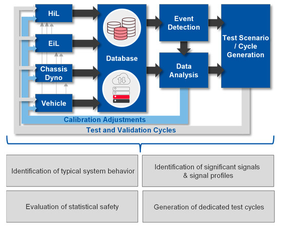
Figure 1.
Schematic overview of the RDE application and validation methodology.
All test environments are used to acquire measurement data. Data analysis by means of event detection and statistical evaluation then refers to the entire database content. The use of the common database enables the continuous use of data from the early phases, focusing on test benches, to the final phases in the vehicle. In addition to, e.g., emission tests or simulations, measurements of daily driving operation (robustness measurements), which represent the real usage behavior of the system, are also stored.
Following the data acquisition and pre-processing for the database layout, an event detection is applied to the data containing an emission measurement trace. The event detection automatically identifies the sequences with increased emission intensities, as described in [43,44]. The rule for the definition of critical intensities and the evaluation of the relevant signals can be adjusted. Thus, the transferability to other topics of interest, such as a hybrid operation strategy, is ensured. Measurements without an emission trace are used for statistical analysis; they can help to prioritize the events with regard to statistical relevance and to evaluate the variety of existing measurement data [42]. Finally, the results of the data analysis are fed back into the testing iterations by means of dataset optimization. They can be tested in dedicated, vehicle-specific test cycles which are built of the events previously detected and statistically evaluated.
To ensure maximum use of the collected data during the development and especially the calibration process, automated analysis is required. In this way, the main advantage of virtualized calibration tasks—increasing the speed of measurements and data collection—can be exploited. The goal for automated data analysis is to deliver added value to the calibration engineer. The data must be analyzed and visualized in a way that is useful for further evaluation and interpretation by the engineer. Thus, all the benefits of automated analysis should be usable without deep knowledge of data science.
The work packages presented in Figure 1 subdivide the process into Identification of typical system behavior, Identification of significant signals & signal profiles, Evaluation of statistical safety and Generation of dedicated test cycles.
The methodology focused on in this work describes a part of the methods used in the first work package, Identification of typical system behavior. The subtopics of this work package are shown in Figure 2. Following this requirement, the process of data analysis should be largely automated within the methodology presented in [42].
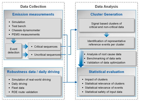
Figure 2.
Schematic overview of data analysis steps.
Using emission calibration as an example, automatic event detection is applied to the measurement data to identify sequences during tests that exhibit increased emission intensity. To further reduce the individual evaluation effort, the events are then processed into clusters. Here, similar events are categorized into groups, which then can be analyzed by the engineer. In this way, not every single event requires evaluation: only reference events of the cluster itself require evaluation. In addition, this allows for the calculation of the overall impact of a weak spot by summarizing the intensity, amount, and statistical relevance. The approach for clustering data will be discussed in its fundamentals in the context of vehicle application within this paper.
In addition to the reduced evaluation effort, with the results of the Identification of typical system behavior (Figure 1) an analysis of relevant signals and root causes becomes possible by using clusters. Cluster comparisons can be used in the Identification of significant signals & signal profiles (Figure 1) to specifically identify cluster occurrences of patterns within critical versus not-critical data clusters, as described in [42]. Since the validation process of cycle generation and emission verification is highly dependent on the available data diversity as a source for critical behavior, an assessment of the data variation quality is performed in the Evaluation of statistical safety (Figure 1). Finally, the data are used for the generation of vehicle-specific test cycles, as further described in [45] and in [42] with an updated approach.
As the events show a high diversity of duration and characteristics, a direct comparison of signal traces is not possible. To overcome slight differences in the shapes and durations of the signals, a dynamic-time-warping (DTW) [46,47] approach is used to compare signals of different events. The distance between the reference signal of the event on which the clustering shall be based is then compared with all other events. Thus, a distance matrix is created, showing the distances for any event combination. The clustering approach shall then group all events with similar traces.
To evaluate the clustering results, different measures are used. The first measure is the Silhouette Score (1). As an intensive measure, it does not require any additional information and is capable of judging the cluster results based only on the categorization. It describes the ratio of similarity within a single cluster and the difference towards the others. This is achieved by using the cohesion for similarity and the separation for differences:
The silhouette is calculated for each element . Finally, the Silhouette Score is the average silhouette over all elements within the cluster. It results in 0 in the case in which there is only one element in the cluster. The cohesion expresses the average distances of all elements within a cluster; the smaller is, the more compact the cluster is. The separation is understood as the average distance of all elements of the neighbor cluster to the element ; high values of express a high separation. [48]
3. Results
Depending on the type and size of the data as well as the specific goal to be achieved, different methods for data clustering can be applied. The choice of method depends on the existing knowledge of the available data and the parameters required for the method. In the example of emission calibration, the signals of interest may have many different and complex structures and characteristics. It is difficult to make assumptions in advance about the number, size, or shape of clusters because the weak spots are highly dependent on the vehicle and the dataset currently being used. To add value to the vehicle calibration evaluation process, the clustering approach must be adaptable with little effort from project to project or use case to use case given the wide variation in data.
In the context of investigating different clustering approaches, hierarchical, partitioning, and density-based clustering methods are evaluated. Fourier-transformation-based methods [49,50,51] previously showed inadequate results due to the often small number of data points within a single event. For usability in the calibration process, clustering results are evaluated in terms of compactness and differentiability, as well as the required prior knowledge of the data. During the investigation, different signals are used as a reference for the calculation of event-to-event distances and thus the clustering itself. This methodology shall be applicable on all kinds of signals to identify significant event groups based on any signal. Later, investigations shall be carried out to identify the characteristic features of a dataset or cluster and will be published in a separate paper. Here, each set of clusters is based on the comparison of a single signal.
3.1. Hierarchical Clustering
Hierarchical clustering is often used for the categorization of time-based data. Empirical analyses show that the results of this methodology are usually of high quality [52,53,54,55]. One of the main advantages is the lack of a need for parameters to create the clusters. Furthermore, a complete cluster structure is created by the algorithm. The resulting hierarchy provides initial information about the dataset. For hierarchical cluster methodologies, there are different approaches to create the clusters. Figure 3 shows an overview of different approaches for hierarchical clustering.
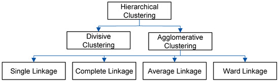
Figure 3.
Overview of approaches for hierarchical clustering.
For hierarchical clustering, a criterion that defines the distance between clusters is required. In addition to the selection of the algorithm for merging events and sub-clusters, the distance measure also has a major impact on the clustering results. As a main principle, the methodologies categorize events with the closest distance from each other into clusters. Neighboring events are combined into clusters at the first step. The clusters are then successively merged as long as the distance between two clusters is below a defined threshold.
For the clustering of emission data, four algorithms—Single Linkage, Complete Linkage, Average Linkage, and Ward Linkage—are used. As a source, an event database consisting of critical events for HC emissions (identified based on the approach described in [44]) is used. The clustering is applied to the engine speed signal.
Single Linkage and Complete Linkage use only one element of each cluster to calculate the distance between two clusters. In contrast, Average Linkage and Ward Linkage use all the elements within the two clusters. To create hierarchical clusters, the distance of the events must be known as a stopping rule. In this case, the distance and the number of useful clusters is unknown. For this reason, the Silhouette Score for to clusters is calculated to experimentally investigate an appropriate distance for the emission events. Similar results were observed on further analyses with different signals and events. The results—expressed by the Silhouette Score—are shown in Figure 4.
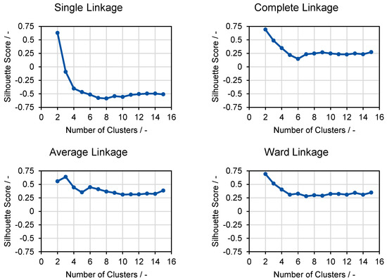
Figure 4.
Silhouette Score results for hierarchical clustering approaches.
The results for Complete Linkage and Ward Linkage on the right (Figure 4) show similar results, whereas Single Linkage shows very different results—even demonstrating negative values as the number of clusters increases. The negative results on higher amounts of clusters for Single Linkage indicate inconsistencies at the low levels of the created hierarchical structure (the first steps of combining events into clusters).
The hierarchical creation of clusters does not allow for the later correction of the lower levels. This leads to the phenomenon that mismatches on a low level have a continuous impact on propagating cluster creation, which leads to inhomogeneous results. This effect leads to a reduction in the distances between the clusters.
As it only considers single elements from a cluster for the calculation of distances between two clusters, the Single Linkage approach tends to create large clusters with quite different signal traces inside. In contrast to the Single Linkage approach, the other approaches show mainly good correlations toward each other and positive results in the Silhouette Score. These results indicate homogeneous clusters with separation to neighboring clusters at each level of the hierarchy. If the number of clusters is too small, the Silhouette Score increases due to the lack of comparison partners. As the Complete Linkage approach tends to form too many small clusters and Ward Linkage tends to form clusters with the same size, Average Linkage is used for further analyses.
For the generation of hierarchical clusters, the use of stopping rules is required. The stopping rules are used to define the point in the structure at which further clustering should be stopped. As measures to define stopping rules and to identify the optimal number of clusters for a dataset, the Elbow Rule, Silhouette Score, and Clustering Gain approaches are evaluated.
The variance of the cluster content is considered with increasing numbers of clusters, as shown in Figure 5. Using only one cluster results in the highest variance, as all datapoints are included. In opposition to this, the variance is if the number of events equals the number of clusters as each cluster only contains one specific signal trace. The Elbow Rule defines the optimum number of clusters by rating the resulting trace with respect to a change in the gradient. In front of the bending point, the variance strongly decreases, meaning that the clusters are becoming more compact. Beyond this point, the variance in the clusters decreases only slightly, meaning that the compactness of the clusters is only slightly optimized [56,57]. Figure 5 shows the results for cluster analyses with two different signals based on emission events. The comparison of the plots of the accelerator pedal position (left) and the voltage of the downstream lambda sensor (right) shows the difficulties in clearly identifying the results according to the Elbow Rule. The right profile shows an obvious bending point at clusters. The left profile shows a smoother trace and does not allow for the clear identification of the point of the optimal number of clusters. Since the bending point is not pronounced enough for some profiles, determining the ideal point using the Elbow Rule is not always possible.
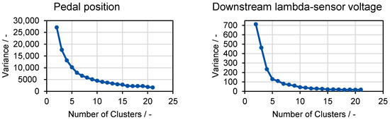
Figure 5.
Definition of optimum cluster amounts using the Elbow Rule.
The Silhouette Score criterion is well-suited for the iterative assessment of the number of clusters. No further information about the data is required, and it is independent of the type of data used for clustering. The application of the Silhouette Score to analyze the cluster quality is shown in Figure 6, using the example of clusters based on the vehicle speed of critical events. While a low number of clusters is desired to best support data analysis, a minimum number of clusters is required to build clusters that adequately represent the characteristics of the signals. With a decreasing number of clusters, the degrees of freedom for separating the data set decrease, resulting in inhomogeneous and large clusters. The local maximum at clusters is thus interpreted as an outlier.

Figure 6.
Definition of optimum cluster amounts using the Silhouette Score for vehicle speed.
The global maximum is reached at clusters. However, the manual evaluation of the resulting clusters shows a number of clusters that is too high. The local maxima at and clusters (Figure 7) show the best results when evaluating the clusters manually. Just as with the Elbow Rule, the Silhouette Score does not show a clear optimum in some cases, which further complicates the use of the Silhouette Score as a decision measure in automated approaches.
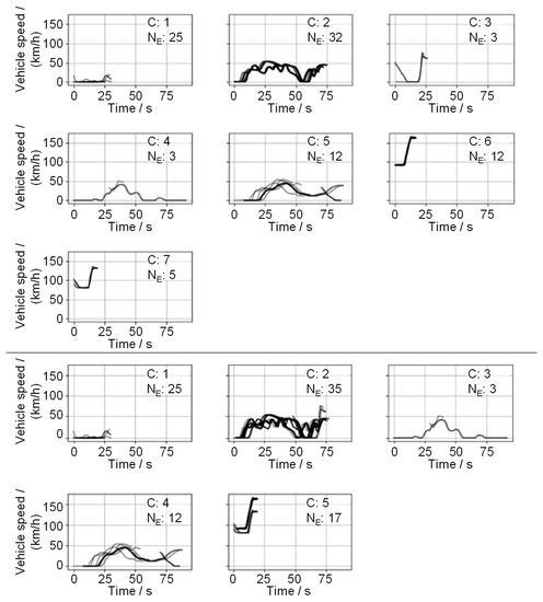
Figure 7.
Hierarchical clustering with 7 (top) and 5 (bottom) target clusters.
Clustering Gain [58] is a measure that evaluates the increase in similarity within the clusters with a decreasing number of clusters compared to a decreasing inner homogeneity. Using Equation (2), the Clustering Gain uses the average distance between all elements within the dataset and the average distance of all elements within a cluster . describes the number of elements within the cluster, and and represent the total number of clusters.
Evaluating different signals of the events shows that the Clustering Gain approach underestimates the number of clusters. A reasonable definition of the optimum number of clusters has shown to work only for a bit signal, which is usually separated in only a small number of clusters. Signal traces with a nearly constant value often represent the average value of several other signal traces that show a higher dynamic within the signal. Such clusters are then combined, leading to the mixing of dynamic and static signal traces. For this reason, signal traces with a low variance and a nearly constant value are separated from the dataset in advance and can then be applied to an individual clustering loop. Figure 8 shows the separation of the static traces of the engine speed. First, the standard deviation is calculated for each signal trace from the events. The percentile that shows a clear jump is determined to define the maximum value of signal variance for static traces. Here, the th percentile is used to separate events with static engine speed traces (Figure 8, right).
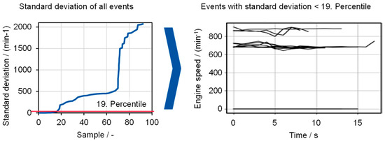
Figure 8.
Separating constant signals from the dataset (right) based on the standard deviation (left).
In general, the Clustering Gain approach offers a good base for the automatic judging of the cluster hierarchy, although the result is highly dependent on the type and characteristics of the signals used. Filtering is required to use the Clustering Gain approach as a measure of the cluster number.
On one hand, hierarchical clustering can be easily applied to arbitrary signals since it does not require signal-specific parameters. Furthermore, the method is applicable to large datasets, and the computed hierarchy helps to explore the dataset structure. On the other hand, the inflexible assignment and errors in low levels of the hierarchy cause the clusters to become inhomogeneous and the distances between individual clusters to become smaller. Another disadvantage is the complex extraction of the final clusters from the hierarchy and the determination of the cluster number. Although approaches such as the Silhouette Score and Clustering Gain can determine the optimal number of clusters, this must be done manually and iteratively for most signals.
3.2. Partitioning Cluster Methodologies
The K-Means algorithm [59,60,61] is a widely used partitioning method. The algorithm optimizes an initial partitioning of a dataset based on a cost function. The advantage of K-Means is that elements can change their cluster, and an optimal partitioning of the dataset is therefore possible.
The algorithm is scalable on large datasets and always converges, whereas the solution can be a local minimum. The selection of the initial partitioning can be generated manually or randomly. Since manual partitioning requires a large amount of effort, multiple partitions are used in this analysis. Several random initializations of the algorithm are examined, and the best result is considered. Only the determination of one parameter (cluster number) is necessary for the K-Means algorithm. For the cluster centers, synthetic traces are used which average all events in the cluster.
The calculation of the cluster center is essential for the optimal assignment of the individual signal traces. The cluster center serves as a representation of the complete cluster and must therefore reflect as many characteristics of the cluster elements as possible. Therefore, the average trace for the clustering is chosen to be the Barycenter, according to [62]. The Barycenter is a synthetic progression that is calculated using DTW. Figure 9 shows the comparison of two mean trajectories for the same cluster. The cluster consists of similar signal traces for the engine speed from critical emission events.

Figure 9.
Calculation of a cluster’s mean trajectory.
In contrast to the simple averaging of the signals (Figure 9, left), the Barycenter of the signals (Figure 9, right) can compensate the local temporal signal waveforms. Thus, the Barycenter maps the entire cluster better than simple averaging and allows for a more accurate mapping. The flexibility of DTW leads to a difference in length between the simple averaging and the Barycenter. In addition to synchronization, the averaging of signals of different lengths is another advantage of the Barycenter. Thus, the Barycenter reproduces the core information of the cluster and is later able to represent the main characteristic of the feature.
As a partitioning method, K-Means requires the specification of the number of clusters, which is not known in advance for the signals from emission events. Therefore, two methods for determining the cluster number are investigated. On one hand, an iterative evaluation of the results is analyzed, and on the other hand, hierarchical clustering is used to determine the cluster number.
As a standard criterion for the evaluation of cluster results, the Silhouette Score is used for an iterative determination of the number of clusters. The optimal partitioning is determined by evaluating the cluster results for different cluster numbers and selecting the highest Silhouette Score result. The optimal partitioning is not always achieved at the absolute maximum value of the Silhouette Score. Cluster numbers that do not show the maximum in the trace of the Silhouette Score can provide better results than numbers that show a maximum Silhouette Score. The Silhouette Score for different target cluster numbers is shown in Figure 10, using the engine torque signal as reference.
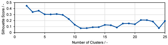
Figure 10.
Silhouette Score for partitioning clustering on engine torque with target number variation.
Figure 11 shows a comparison of the clustering results of events, sorted into (top) and clusters (bottom). The cluster number is usually underestimated, making the clusters inhomogeneous.
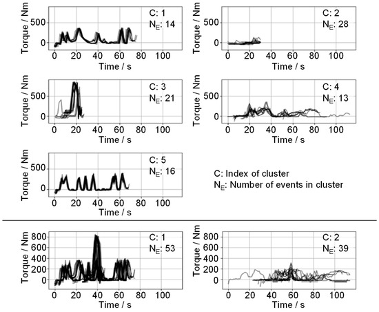
Figure 11.
Comparison of cluster results for event torque using 5 clusters (top) versus 2 clusters (bottom).
Clustering Gain can automatically determine the number of clusters in the hierarchical clustering. However, the rigid assignment of the data points leads to inhomogeneous clusters. K-Means allows for a flexible assignment and can optimize the clusters. For this purpose, the clusters determined using the Clustering Gain approach are used as initial partitioning for the K-Means algorithm. However, the investigations using a combined approach of K-Means and Clustering Gain generally do not achieve a significant improvement in the generated clusters. K-Means is not able to perform the partitioning due to the underestimation of the number of clusters by the Clustering Gain algorithm.
Due to the possibility of exchanging data points between the clusters and the minimization of the average distance within the clusters, the K-Means algorithm forms homogeneous clusters when the optimal cluster number is known. However, the determination of the cluster number for emission events cannot be automated reliably for all signals. Furthermore, K-Means tries to partition the complete dataset and has no possibility of detecting outliers.
3.3. Density-Based Clustering
The hierarchical density-based clustering methodology HDBSCAN combines the advantages of hierarchical and partitioning approaches. First, a hierarchy is created. Then, an optimization algorithm adjusts the clusters by judging the density of the different branches of the hierarchy. This approach enables a hybrid cluster generation process that does not require information about the desired number of clusters. One of the advantages of this technology is its ability to automatically identify outliers in the data. This prevents the mismatch of clusters when trying to sort outliers into the actual patterns. For control of the HDBSCAN methodology, the two key parameters, minimal cluster size and minimal density need to be defined [63].
The minimal cluster size defines the number of samples (events) that at least need to be assigned to a cluster. Thus, only dense areas with at least data points are considered for the creation of clusters. Small values for are favored to consider as many points as possible, whereas values that are too small will lead to the overfitting of single clusters and subsequently to the creation of many rather small clusters.
The minimal density describes the characteristic of the area that shall be considered for clustering. A minimal number of samples in a specific area is required to consider this area for the generation of clusters. An area that is not dense enough will not be considered for the generation of clusters. The smaller the number, the more events will be considered for the formation of clusters. A value that is too high will exclude a high number of events and will cause only extremely dense areas to be considered, while a number that is too low will enable the consideration of even outliers and thus might falsify or negatively influence the compactness of the clusters.
To identify the influence of both parameters on the clustering of emission events, further analyses are carried out. Test datasets built of critical emission events are created for different exhaust emission components, whereas different numbers of events are used for each (Table 1).

Table 1.
Number of events per dataset per emission component.
emission-relevant signals are selected as base for the clustering approach listed in Table 2. These signals were selected as samples for signals with both a known influence on the emission intensity and different characteristics. Here, signals with a bit characteristic (bit fuel cut-off) and high (engine torque and downstream lambda sensor voltage) and low (e.g., vehicle speed and temperature of catalytic converter) dynamics and ranges are used. The HDBSCAN parameters and are varied to identify the best cluster setup with the least number of outliers. Judgement is carried out by means of the Silhouette Score and visual evaluation. An overview of the selected parameter combinations for the signals is provided for each of the evaluated emission components in Table 3. The generation of clusters is always based on one signal, creating a set of clusters for each of the listed signal and emission component combinations.
Table 2.
Overview of HDBSCAN parameter evaluation with averaged results.
Table 3.
Overview of results of the HDBSCAN parameter variation.
Silhouette Score values of represent good results of the HDBSCAN. Here, the number of clusters is not underestimated, and a good fit is shown. For all investigated signals, such a score could be achieved when evaluating the averaged results over all six emission components. The values for and used to achieve the results are listed in Table 3. The quality of the results appears to be independent of the signal and the size of the dataset (Table 1). For signals with low dynamics (e.g., temperature of the catalytic converter), the share of outliers is rather low. Signals with a high share of detected outliers are indicated mainly by those with different levels with respect to their absolute value. For such signals, the algorithm could be re-applied to the events classified as outliers with an adjusted parameter set to regroup events of different magnitudes.
The identified best-fitting values for range from to , regardless of the size of the dataset. out of signals reach the optimum for . Exceptions are only observed for signals with low noise in their profile and the presence of ideal clusters.
The parameter for the minimal density shows a good correlation with the minimal cluster size. The absolute differences of and are shown in Figure 12 as a histogram and boxplot. For out of sets, and result in the same value. For the majority of differences, the value can be rather neglected. Here, the 75th percentile has a value of , while the 25th percentile and median are both expressed by a difference of . High differences can be considered as outliers (judging both the 97.5th percentile or the interquartile range). In addition, further variations of with a constant around the optimum value of are shown to have a neglectable effect.
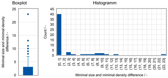
Figure 12.
Evaluation of and differences.
Since the minimum density and minimum cluster size parameters are mostly the same, the parameters are set as equal for further application. This allows for the reduction of the input parameters for HDBSCAN to a single parameter.
The methodology used to create the resulting clusters is a further influencing factor for the HDBSCAN procedure. Clustering can either be performed following the Excess of Mass or the leaf rule. As the standard methodology, Excess of Mass shows a tendency to create a smaller number of clusters with a large size. On the other hand, leaf generates small, homogeneous clusters in larger numbers while also allowing for the formation of large clusters if they are present in a homogeneous layout. Since signals for emission events and for vehicle measurements generally have a high variation in their characteristics, the generation of smaller clusters is preferred in this context. Following the leaf method, a larger number of clusters is chosen for use in emission calibration, which can then be concatenated.
With the combination of small values for and the leaf methodology, the process of concatenating micro-clusters directly is supported by a limit of minimal distance between clusters. The can be used to define the distance between two clusters. Single clusters with a distance smaller than this will be automatically joined.
In summary, HDBSCAN is a reliable method for categorizing emission critical events into clusters of different sizes. The method identifies the typical traces of different signals. As it is independent of the signal traces, the method can be applied to different signal characteristics and can even categorize static traces into separate clusters. By being able to reduce the control parameters to a single factor, its application in the context of a vehicle application offers a promising base. A tendency to form micro-clusters can be observed, but this can be countered by combining multiple micro-clusters using .
4. Discussion
Section 3 demonstrates the applications of three different approaches to clustering data.
For hierarchical clustering, the Average Linkage procedure is the best compromise between many small clusters and a few larger ones. An advantage of hierarchical clustering is the small number of required settings. Only a threshold value for the distance to combine neighboring clusters with each other as stopping rule is required, which is challenging to define in the context of vehicle calibration with different signals of interest as there can be a high variety of signals. During the investigation, different approaches are evaluated to provide an automatic procedure to help the engineer to define this stopping rule. Comparing the Elbow Rule, the Silhouette Score, and the Clustering Gain, all measures show disadvantages in being applied to different signals.
As result, hierarchical clustering is an easy application for different signals and is a reliable procedure even for large datasets. However, for daily use in the context of vehicle calibration, the required pre-evaluation of the signals is a major challenge. The evaluation of the data characteristics exceeds the typical analysis procedures of calibration engineers and is therefore not easy to adopt.
Using partitioning clustering with the K-Means approach shows a similar disadvantage to what is observed for hierarchical clustering. As a control value, the number of clusters to be created must be defined. Due to the wide variety of signal types and traces within the calibration process, a standard target cannot be assigned easily.
Similar to hierarchical clustering, the high variance of signals of interest during the calibration process leads to a necessary pre-evaluation of the data. Finding the optimal number of clusters as a control value for the algorithm proves to be signal-dependent and challenging.
The HDBSCAN approach is evaluated as a density-based clustering methodology. Here, the variance of the two control parameters, minimal cluster size and minimal density, shows that equal values can be set for both parameters.
Using the leaf method as a clustering algorithm shows that smaller clusters are created in greater numbers. In contrast, the Excess of Mass methodology creates only fewer but larger clusters. During the analysis and evaluation process, it is observed that a larger number of smaller clusters is preferable. Here, the combination of individual clusters can be easily performed during their visual examination. In addition, is used to define the distance between two clusters as a threshold value below which two clusters are to be combined automatically. An iteration of this threshold can be used after a brief visual examination to reduce the number of clusters automatically if required and if reasonable.
The HDBSCAN shows reliable results for different types of signals with different characteristics. The combination of hierarchy-based clustering and the optimization of the results similar to the partitioning approach proves to be the most flexible of the investigated approaches. In contrast to pure hierarchical clustering, the distance used as a stopping rule is not applied globally but only locally. Each combination of clusters within the hierarchy is evaluated regarding the change in density of the clusters and their surrounding area. As long as a combination of clusters leads to a higher separation of clusters from their environment, the combination is performed. The stopping rule is adjusted for each branch.
The ability to consider outliers provides the advantage of not falsifying clusters by trying to sort in all the events. Especially in emission testing, outliers can be caused by the behavior of measurement equipment, environmental impacts, or even signal synchronization. Comparing the effort of parameter identification, HDBSCAN has an acceptable scope in the calibration process. For the most part, the evaluation of reasonable parameters can be performed in an iterative, automatic manner. Only a small amount of data science knowledge and experience with the approaches is required to evaluate the resulting cluster characteristics.
5. Conclusions
New technologies and approaches are being integrated into the vehicle development process to reduce exhaust emissions and address climate change. The use of virtual calibration approaches in RDE optimization and validation can offer major benefits in terms of the safety of different scenarios and speed of testing. However, to make the most of these approaches, the data processing and analysis itself must also be optimized.
In order to better utilize the large amount of data required for RDE testing, a methodology for the automatic pre-analysis of data is introduced. Using the results of previously developed event-detection procedures [43,44], clustering algorithms are utilized to categorize and presort events. This paper discusses the fundamentals of various clustering approaches in the vehicle calibration process.
Hierarchical, partitioning, and density-based clustering methods are evaluated. For a sustainable implementation in the calibration process, the appropriate method must be reliable for different signal types, have a high degree of automation, and require little knowledge about the data and control values.
Both the hierarchical and partitioning approaches show good results in terms of clustering when the database is well-known. However, with highly varying signal types and unknown populations of events, neither the desired number of clusters nor a maximum spacing of signals to form the clusters is known. Intensive manual data analyses are required to identify the necessary control parameters. As a combination, the density-based clustering approach shows the greatest potential.
As a density-based approach, the HDBSCAN algorithm is used. The analysis shows that the two control parameters, minimum cluster size and minimum density, can be set to the same value, reducing the required inputs. Combining this with the leaf method allows for the creation of a higher number of compact clusters of a rather small size.
Clustering data with this approach can significantly reduce the manual effort required for data analysis. As there is no need to evaluate all events, the automatic categorization of events provides added value for the calibration engineer. The focus can be on the central events of a cluster. In addition, having numerous events with similar signal characteristics simplifies a root cause analysis. Further, the impact of a single weak spot can be quantified. The quantification of the weak spots themselves provides a tool for benchmarking calibrations of different datasets or vehicles.
While this paper presents the basic principles for identifying suitable clustering methods, further research will discuss the application of the clustering methods within the calibration process itself. Implementation of density-based clustering in the calibration process will allow for further validation of the methodology with additional data. For future application, the approach can be transferred to other technologies. Events and clusters regarding consumption optimization or thermal management and derating can be implemented for electrified vehicles. For fuel cell vehicles, automated analyses regarding cold start behavior and humidity management as well as aging behavior are feasible. Data will be automatically accounted for so that even minor anomalies are assessed for their overall impact, whereas the current manual approach tends to focus on high-intensity outliers.
Author Contributions
Conceptualization, S.K. and J.C.; methodology, S.K. and G.T.; software, G.T.; validation, S.K. and G.T.; formal analysis, S.K. and G.T.; investigation, S.K. and G.T.; resources, S.K. and S.P.; data curation, S.K. and J.C.; writing—original draft preparation, S.K.; writing—review and editing, J.C., G.T., M.D., F.D. and S.P.; visualization, S.K. and G.T.; supervision, S.P.; project administration, S.K.; funding acquisition, S.P. All authors have read and agreed to the published version of the manuscript.
Funding
The presented research was carried out at the Center for Mobile Propulsion (CMP) of RWTH Aachen University, funded by the German Science Council “Wissenschaftsrat” (WR) and the German Research Foundation “Deutsche Forschungsgemeinschaft” (DFG).
Data Availability Statement
The data presented in this study are available on request from the corresponding author. The data are not publicly available due to the complexity of the analysis which needs guidance for reproduction and confidentiality of root measurements.
Conflicts of Interest
The authors declare no conflict of interest. The funders had no role in the design of the study; in the collection, analyses, or interpretation of data; in the writing of the manuscript, or in the decision to publish the results.
References
- European Commission. The European Green Deal: Communication from the Commission to the European Parliament, the European Council, the Council, the European Economic and Social Committee and the Committee of the Regions. 2019. Available online: https://eur-lex.europa.eu/legal-content/EN/TXT/?uri=celex%3A52019DC0640 (accessed on 28 March 2023).
- Maurer, R.; Yadla, S.K.; Balazs, A.; Thewes, M.; Walter, V.; Uhlmann, T. Designing Zero Impact Emission Vehicle Concepts. In Experten-Forum Powertrain: Ladungswechsel und Emissionierung; Liebl, J., Ed.; Springer: Berlin/Heidelberg, Germany, 2020; ISBN 978-3-662-63523-0:75–116. [Google Scholar]
- Mulholland, E.; Miller, J.; Braun, C.; Jin, L.; Rodríguez, F. Quantifying the long-term air quality and health benefits from Euro 7/VII standards in Europe. Int. Counc. Clean Transp. 2021. [Google Scholar]
- Baumgarten, H.; Görgen, M.; Balazs, A.; Nijs, M. New Lambda = 1 Gasoline Powertrains New Technologies and Their Interaction with Connected and Autonomous Driving. In Proceedings of the 30th International AVL Conference Engine & Environment, Graz, Austria, 7–8 June 2018. [Google Scholar]
- Sterlepper, S.; Claßen, J.; Pischinger, S.; Görgen, M.; Cox, J.; Nijs, M.; Schraf, J. Relevance of Exhaust Aftertreatment System Degradation for EU7 Gasoline Engine Applications; SAE Technical Paper 2020-01-0382, 2020; SAE International 400 Commonwealth Drive: Warrendale, PA, USA, 21 April 2020. [Google Scholar] [CrossRef]
- European Commission. Commission Regulation (EU) 2017/1151. 2017. Available online: http://publications.europa.eu/resource/cellar/7d1c640d-62d8-11e7-b2f2-01aa75ed71a1.0006.02/DOC_1 (accessed on 28 March 2023).
- Europäischen Union. Verordnung (EU) 2019/631 des Europäischen Parlaments und des Rates; Europäischen Union: Maastricht, The Netherlands, 2019. [Google Scholar]
- European Commission. Proposal for a Regulation of the European Parliament and of the Council on Type-Approval of Motor Vehicles and Engines and of Systems, Components and Separate Technical Units Intended for Such Vehicles, with Respect to Their Emissions and Battery Durability (Euro 7) and Repealing Regulations (EC) No 715/2007 and (EC) No 595/2009. 2022, Volume 0365. Proposal. Available online: https://eur-lex.europa.eu/legal-content/EN/TXT/?uri=CELEX%3A52022PC0586 (accessed on 28 March 2023).
- Boger, T.; Rose, D.; He, S.; Joshi, A. Developments for future EU7 regulations and the path to zero impact emissions—A catalyst substrate and filter supplier’s perspective. Transp. Eng. 2022, 10, 100129. [Google Scholar] [CrossRef]
- Claßen, J.; Krysmon, S.; Dorscheidt, F.; Sterlepper, S.; Pischinger, S. Real Driving Emission Calibration—Review of Current Validation Methods against the Background of Future Emission Legislation. Appl. Sci. 2021, 11, 5429. [Google Scholar] [CrossRef]
- Maurer, R.; Kossioris, T.; Hausberger, S.; Toenges-Schuller, N.; Sterlepper, S.; Günther, M.; Pischinger, S. How to define and achieve Zero-Impact emissions in road transport? Transp. Res. Part D Transp. Environ. 2023, 116, 103619. [Google Scholar] [CrossRef]
- Görgen, M.; Nijs, M.; Thewes, M.; Balazs, A.; Yadla, S.K.; Scharf, J.; Uhlmann, T.; Claßen, J.; Dorscheidt, F.; Krysmon, S.; et al. Holistic Hybrid RDE Calibration Methodology for EU7. Int. Mot. 2021, 189–215. [Google Scholar] [CrossRef]
- Maurer, R.; Kossioris, T.; Sterlepper, S.; Günther, M.; Pischinger, S. Achieving Zero-Impact Emissions with a Gasoline Passenger Car. Atmosphere 2023, 14, 313. [Google Scholar] [CrossRef]
- Dorscheidt, F.; Pischinger, S.; Claßen, J.; Sterlepper, S.; Krysmon, S.; Görgen, M.; Nijs, M.; Straszak, P.; Abdelkader, A.M. Development of a Novel Gasoline Particulate Filter Loading Method Using a Burner Bench. Energies 2021, 14, 4914. [Google Scholar] [CrossRef]
- Xia, F.; Dorscheidt, F.; Lücke, S.; Andert, J.; Gardini, P.; Scheel, T.; Walter, V.; Tharmakulasingam, J.K.R.; Böhmer, M.; Nijs, M. Experimental Proof-of-Concept of HiL Based Virtual Calibration for a Gasoline Engine with a Three-Way-Catalyst. 2019 JSAE/SAE Powertrains Fuels Lubr. 2019. [Google Scholar] [CrossRef]
- Picerno, M.; Lee, S.-Y.; Ehrly, M.; Schaub, J.; Andert, J. Virtual Powertrain Simulation: X-in-the-Loop Methods for Concept and Software Development. In Proceedings of the 21st Internationales Stuttgarter Symposium, Stuttgart, Germany, 30–31 March 2021; Bargende, M., Reuss, H.-C., Wagner, A., Eds.; Springer Fachmedien Wiesbaden: Wiesbaden, Germany, 2021. ISBN 978-3-658-33465-9:531–545. [Google Scholar] [CrossRef]
- Krysmon, S.; Bonnaventure, R.; de Baroud, W.; Kluge, K. FEV’s modern X-in-the-Loop-Test Benches for Hybrid Powertrains. FEV Spectr. 2020, 71, 40–45. [Google Scholar]
- Nickel, D.; Behrendt, M.; Bause, K.; Albers, A. Connected testbeds—Early validation in a distributed development environment. In 18. Internationales Stuttgarter Symposium; Bargende, M., Reuss, H.-C., Wiedemann, J., Eds.; Springer Fachmedien Wiesbaden: Wiesbaden, Germany, 2018; pp. 1173–1185. ISBN 978-3-658-21193-6. [Google Scholar]
- Lee, S.-Y.; Andert, J.; Neumann, D.; Querel, C.; Scheel, T.; Aktas, S.; Miccio, M.; Schaub, J.; Koetter, M.; Ehrly, M. Hardware-in-the-Loop-Based Virtual Calibration Approach to Meet Real Driving Emissions Requirements; SAE Technical Paper 2018-01-0869, 2018, WCX World Congress Experience; SAE International400 Commonwealth Drive: Warrendale, PA, USA, 10 April 2018. [Google Scholar] [CrossRef]
- Dorscheidt, F.; Düzgün, M.; Claßen, J.; Krysmon, S.; Pischinger, S.; Görgen, M.; Dönitz, C.; Nijs, M. Hardware-in-the-Loop Based Virtual Emission Calibration for a Gasoline Engine. SAE Tech. Pap. 2021. [Google Scholar] [CrossRef]
- Powertrain and Fluid Systems Conference and Exhibition. Emissions: Advanced catalyst and substrates, measurement and testing, and diesel gaseous emissions. In Proceedings of the Powertrain & Fluid Systems Conference & Exhibition, Pittsburgh, PA, USA, 27–30 October 2003; ISBN 0-7680-1319-4.
- Etzold, K.; Scheer, R.; Fahrbach, T.; Zhou, S.; Goldbeck, R.; Guse, D.; Frie, F.; Sauer, D.U.; De Doncker, R.W.; Andert, J. Hardware-in-the-Loop Testing of Electric Traction Drives with an Efficiency Optimized DC-DC Converter Control; SAE Technical Paper 2020-01-0462, WCX SAE World Congress Experience; SAE International400 Commonwealth Drive: Warrendale, PA, USA, 21 April 2020. [Google Scholar] [CrossRef]
- Jiang, S.; Smith, M.H.; Kitchen, J.; Ogawa, A. Development of an Engine-in-the-loop Vehicle Simulation System in Engine Dynamometer Test Cell. SAE Tech. Pap. 2009. [Google Scholar] [CrossRef]
- Guse, D.; Claßen, J.; Kumagai, T.; Ueda, N.; Scharf, J.; Nijs, M.; Balazs, A.; Görgen, M. Powertrain development frontloading for RDE compliance—Part 2: Robust RDE compliant PN emissions calibration at Engine-in-the-Loop test bench. JSAE 2018. [Google Scholar]
- Heusch, C.; Guse, D.; Dorscheidt, F.; Claßen, J.; Fahrbach, T.; Pischinger, S.; Tegelkamp, S.; Görgen, M.; Nijs, M.; Scharf, J. Analysis of Drivability Influence on Tailpipe Emissions in Early Stages of a Vehicle Development Program by Means of Engine-in-the-Loop Test Benches; SAE Technical Paper 2020-01-0373, WCX SAE World Congress Experience; SAE International400 Commonwealth Drive: Warrendale, PA, USA, 21 April 2020. [Google Scholar] [CrossRef]
- Heusch, C.; Pischinger, S.; Guse, D.; Trampert, S. Objektivierte Fahrbarkeitsuntersuchung am Powertrain-in-the-Loop-Prüfstand. Mtzextra 2021, 26, 24–29. [Google Scholar] [CrossRef]
- Wasserburger, A.; Didcock, N.; Hametner, C. Efficient real driving emissions calibration of automotive powertrains under operating uncertainties. Eng. Optim. 2021, 55, 140–157. [Google Scholar] [CrossRef]
- Maschmeyer, H. Systematische Bewertung Verbrennungsmotorischer Antriebssysteme Hinsichtlich Ihrer Realfahrtemissionen am Motorenprüfstand. Ph.D. Thesis, TU Darmstadt, Darmstadt, Germany, 2017. [Google Scholar]
- Baumgarten, H.; Scharf, J.; Thewes, M.; Uhlmann, T.; Balazs, A.; Böhmer, M. Simulation-Based Development Methodology for Future Emission Legislation. In Proceedings of the 37th Internationales Wiener Motorensymposium, 28–29 April 2016. [Google Scholar]
- Böhmer, M. Simulation der Abgasemissionen von Hybridfahrzeugen für Reale Fahrbedingungen. Ph.D. Thesis, Rheinisch-Westfälische Technische Hochschule Aachen, Aachen, Germany, 2017. [Google Scholar]
- Roberts, P.J.; Mumby, R.; Mason, A.; Redford-Knight, L.; Kaur, P. RDE Plus—The Development of a Road, Rig and Engine-in-the-Loop Test Methodology for Real Driving Emissions Compliance; SAE Technical Paper 2019-01-0756, WCX SAE World Congress Experience; SAE International400 Commonwealth Drive: Warrendale, PA, USA, 9 April 2019. [Google Scholar] [CrossRef]
- Roberts, P.; Mason, A.; Whelan, S.; Tabata, K.; Kondo, Y.; Kumagai, T.; Mumby, R.; Bates, L. RDE Plus—A Road to Rig Development Methodology for Whole Vehicle RDE Compliance: Overview; SAE Technical Paper 2020-01-0376, WCX SAE World Congress Experience; SAE International400 Commonwealth Drive: Warrendale, PA, USA, 21 April 2020. [Google Scholar]
- Donateo, T.; Giovinazzi, M. Building a cycle for Real Driving Emissions. Energy Procedia 2017, 126, 891–898. [Google Scholar] [CrossRef]
- Kondaru, M.K.; Telikepalli, K.P.; Thimmalapura, S.V.; Pandey, N.K. Generating a Real World Drive Cycle–A Statistical Approach; SAE Technical Paper 2018-01-0325, WCX World Congress Experience; SAE International400 Commonwealth Drive: Warrendale, PA, USA, 10 April 2018. [Google Scholar] [CrossRef]
- Balau, A.E.; Kooijman, D.; Rodarte, I.V.; Ligterink, N. Stochastic Real-World Drive Cycle Generation Based on a Two Stage Markov Chain Approach. SAE Int. J. Mater. Manuf. 2015, 8, 390–397. [Google Scholar] [CrossRef]
- Ashtari, A.; Bibeau, E.; Shahidinejad, S. Using Large Driving Record Samples and a Stochastic Approach for Real-World Driving Cycle Construction: Winnipeg Driving Cycle. Transp. Sci. 2014, 48, 170–183. [Google Scholar] [CrossRef]
- Forster, D.; Inderka, R.B.; Gauterin, F. Data-Driven Identification of Characteristic Real-Driving Cycles Based on k-Means Clustering and Mixed-Integer Optimization. IEEE Trans. Veh. Technol. 2019, 69, 2398–2410. [Google Scholar] [CrossRef]
- Wasserburger, A.; Hametner, C. Automated Generation of Real Driving Emissions Compliant Drive Cycles Using Conditional Probability Modeling. In Proceedings of the 2020 IEEE Vehicle Power and Propulsion Conference (VPPC), Gijon, Spain, 18 November–16 December 2020; IEEE: Piscataway, NJ, USA. ISBN 978-1-7281-8959-8:1–6. [Google Scholar]
- Millo, F.; Piano, A.; Zanelli, A.; Boccardo, G.; Rimondi, M.; Fuso, R. Development of a Fully Physical Vehicle Model for Off-Line Powertrain Optimization: A Virtual Approach to Engine Calibration; SAE Technical Paper 2021-24-0004, 15th International Conference on Engines & Vehicles; SAE International400 Commonwealth Drive: Warrendale, PA, USA, 12 September 2021. [Google Scholar] [CrossRef]
- Meli, M.; Pischinger, S.; Gärtner, J. Neural Network based ECU Software Function Representation and Optimization for Base Calibration of Internal Combustion Engines. In Proceedings of the 10. International Conference on Modeling and Diagnostics for Advanced Engine Systems, Sapporo, Japan, 5–8 July 2022. [Google Scholar]
- Meli, M.; Pischinger, S.; Kansagara, J.; Dönitz, C.; Liberda, N.; Nijs, M. Proof of Concept for Hardware-in-the-Loop Based Knock Detection Calibration; SAE Technical Paper 2021-01-0424, SAE WCX Digital Summit; SAE International400 Commonwealth Drive: Warrendale, PA, USA, 13 April 2021. [Google Scholar] [CrossRef]
- Krysmon, S.; Dorscheidt, F.; Claßen, J.; Düzgün, M.; Pischinger, S. Real Driving Emissions—Conception of a Data-Driven Calibration Methodology for Hybrid Powertrains Combining Statistical Analysis and Virtual Calibration Platforms. Energies 2021, 14, 4747. [Google Scholar] [CrossRef]
- Claßen, J. Entwicklung statistisch relevanter Prüfszenarien zur Bewertung der Fahrzeug-Emissionsrobustheit unter realen Fahrbedingungen. Ph.D. Thesis, Universitätsbibliothek der RWTH, Aachen, Germany, 2022. [Google Scholar] [CrossRef]
- Claßen, J.; Pischinger, S.; Krysmon, S.; Sterlepper, S.; Dorscheidt, F.; Doucet, M.; Reuber, C.; Görgen, M.; Scharf, J.; Nijs, M.; et al. Statistically supported real driving emission calibration: Using cycle generation to provide vehicle-specific and statistically representative test scenarios for Euro 7. Int. J. Engine Res. 2020, 21, 1783–1799. [Google Scholar] [CrossRef]
- Claßen, J.; Sterlepper, S.; Dorscheidt, F.; Görgen, M.; Scharf, J.; Nijs, M.; Alt, N.; Balazs, A.; Böhmer, M.; Doucet, M.; et al. RDE cycle generation—A statistical approach to cut down testing effort and provide a secure base to approve RDE legislation compliance. Int. Mot. 2019, 76, 37–56. [Google Scholar] [CrossRef]
- Salvador, S.; Chan, P. Toward accurate dynamic time warping in linear time and space. Intell. Data Anal. 2007, 11, 561–580. [Google Scholar] [CrossRef]
- Serrà, J.; Arcos, J.L. An empirical evaluation of similarity measures for time series classification. Knowledge-Based Syst. 2014, 67, 305–314. [Google Scholar] [CrossRef]
- Rousseeuw, P.J. Silhouettes: A graphical aid to the interpretation and validation of cluster analysis. J. Comput. Appl. Math. 1987, 20, 53–65. [Google Scholar] [CrossRef]
- Han, J.; Kamber, M.; Pei, J. Data Mining: Concepts and Techniques, 3rd ed.; Morgan Kaufmann: Burlington, MA, USA, 2012. [Google Scholar] [CrossRef]
- Portnoff, M. Time-frequency representation of digital signals and systems based on short-time Fourier analysis. IEEE Trans. Acoust. Speech Signal Process. 1980, 28, 55–69. [Google Scholar] [CrossRef]
- Mateo, C.; Talavera, J.A. Short-Time Fourier Transform with the Window Size Fixed in the Frequency Domain (STFT-FD): Implementation. Softwarex 2018, 8, 5–8. [Google Scholar] [CrossRef]
- Abanda, A.; Mori, U.; Lozano, J.A. A review on distance based time series classification. Data Min. Knowl. Discov. 2018, 33, 378–412. [Google Scholar] [CrossRef]
- Batista, G.E.; Wang, X.; Keogh, E.J. A Complexity-Invariant Distance Measure for Time Series. In Proceedings of the 2011 SIAM International Conference on Data Mining, Mesa, AZ, USA, 28–30 April 2011; Liu, B., Liu, H., Clifton, C., Washio, T., Kamath, C., Eds.; Society for Industrial and Applied Mathematics: Philadelphia, PA, USA, 2011; ISBN 978-0-89871-992-5:699–710. [Google Scholar]
- Petitjean, F.; Forestier, G.; Webb, G.I.; Nicholson, A.E.; Chen, Y.; Keogh, E. Faster and more accurate classification of time series by exploiting a novel dynamic time warping averaging algorithm. Knowl. Inf. Syst. 2015, 47, 1–26. [Google Scholar] [CrossRef]
- Rani, S.; Sikka, G. Recent Techniques of Clustering of Time Series Data: A Survey. Int. J. Comput. Appl. 2012, 52, 1–9. [Google Scholar] [CrossRef]
- Goutte, C.; Toft, P.; Rostrup, E.; Nielsen, F.; Hansen, L.K. On Clustering fMRI Time Series. Neuroimage 1999, 9, 298–310. [Google Scholar] [CrossRef]
- Thorndike, R.L. Who belongs in the family? Psychometrika 1953, 18, 267–276. [Google Scholar] [CrossRef]
- Jung, Y.; Park, H.; Du, D.-Z.; Drake, B.L. A Decision Criterion for the Optimal Number of Clusters in Hierarchical Clustering. J. Glob. Optim. 2003, 25, 91–111. [Google Scholar] [CrossRef]
- Ahmed, M.; Seraj, R.; Islam, S.M.S. The k-means Algorithm: A Comprehensive Survey and Performance Evaluation. Electronics 2020, 9, 1295. [Google Scholar] [CrossRef]
- Wiedenbeck, M.; Züll, C. Klassifikation mit Clusteranalyse: Grundlegende Techniken hierarchischer und K-means-Verfahren. GESIS-How-10 2001. [Google Scholar]
- Na, S.; Xumin, L.; Yong, G. Research on k-means Clustering Algorithm: An Improved k-means Clustering Algorithm. In Proceedings of the 2010 Third International Symposium on Intelligent Information Technology and Security Informatics, Jian, China, 2–4 April 2010; IEEE: Piscataway, NJ, USA, 2011. ISBN 978-1-4244-6730-3:63–67. [Google Scholar]
- Petitjean, F.; Ketterlin, A.; Gançarski, P. A global averaging method for dynamic time warping, with applications to clustering. Pattern Recognit. 2011, 44, 678–693. [Google Scholar] [CrossRef]
- McInnes, L.; Healy, J.; Astels, S. hdbscan: Hierarchical density based clustering. J. Open Source Softw. 2017, 2, 205. [Google Scholar] [CrossRef]
Disclaimer/Publisher’s Note: The statements, opinions and data contained in all publications are solely those of the individual author(s) and contributor(s) and not of MDPI and/or the editor(s). MDPI and/or the editor(s) disclaim responsibility for any injury to people or property resulting from any ideas, methods, instructions or products referred to in the content. |
© 2023 by the authors. Licensee MDPI, Basel, Switzerland. This article is an open access article distributed under the terms and conditions of the Creative Commons Attribution (CC BY) license (https://creativecommons.org/licenses/by/4.0/).