1. Introduction
This contribution is motivated by two research projects. The first project deals with the vehicle–track interaction in experiment and theory [
1], the second project deals with the prediction of railway-induced vibration [
2]. In the latter, a user-friendly prediction code has been developed which uses the simplest models with a minimum of parameters that sufficiently yield accurate predictions. In this article, more complex vehicle models are compared with the simplest model of a rigid wheelset to check if special vehicle dynamic effects yield considerable excitation forces for ground vibrations and must be added to the prediction code.
In the project of vehicle–track interaction, a complex measuring campaign was performed at the German high-speed line near Würzburg [
1]. Vehicle, track, and soil vibrations have been measured simultaneously at a surface, bridge, and tunnel line during train runs with specified speeds and impact hammer excitation. The measurement results for the surface line are used here to confirm the theoretical analyses.
Most experimental studies on railway-induced ground vibrations concentrate on the measurements of the ground vibration, for example [
3,
4,
5,
6,
7]. It is now almost a standard to determine the soil properties by wave measurements and analysis, see examples in [
8,
9,
10,
11,
12]. Important additional information is obtained from measured track irregularities as in [
13,
14,
15]. Even better are measurements of the vehicle vibration [
16,
17,
18,
19], namely axle-box measurements, but they are rarely combined with ground vibration measurements [
20].
Vehicle dynamics are usually analysed as multi-body systems [
21,
22,
23]. The simplest models would be multi-degree-of-freedom rigid body models. Much more complex multibody formalisms (including the complex wheel–rail contact mechanism) such as Gensys, SIMPACK, VAMPIRE, and NUCARS are in use to solve problems of running stability and wear [
24]. Flexible vehicle components, namely car bodies [
25] and wheelsets [
26,
27], are modelled for ride comfort, noise reduction, and wear control. These methods are usually too complex for the ground vibration problem. The interaction of the vehicle with the track and the underlying soil, however, is rarely found in vehicle dynamics.
The methods for the dynamics of the track and the train-induced ground vibrations are typically finite element methods with special boundaries [
17,
28], boundary element methods [
11,
29], wavenumber domain methods [
13,
30,
31], and combined finite element and wavenumber methods (the so-called 2.5D method [
14,
15,
32]). These methods allow us to calculate the propagation of waves travelling away from the track. The generation of the waves is often simplified. The interaction of the unsprung vehicle mass and the irregularities of the vehicle and track is widely accepted as excitation. More detailed vehicle models have been analysed for train-induced ground vibrations [
33]. In [
33,
34], the additional influence of the bogie mass has been discussed, but later it has been found that it is of minimal effect [
35]. To conclude, vehicle dynamics have rarely looked at the vehicle forces that generate train-induced ground vibrations [
36], whereas ground vibration specialists have rarely examined the possible vehicle effects on the excitation of waves in the soil.
The aim of the present article is to cover the whole vehicle–track–soil interaction and the induced ground vibration. Vibration measurements of a railway vehicle are evaluated for the forces on the track (and the soil), which excite the ground vibration in the environment. The article is structured as follows: The measurement campaign about vehicle, track and ground vibrations at a surface, bridge, and tunnel line are presented in
Section 2. The results of the vehicle, track, and ground measurements at the surface line are presented for different train speeds in
Section 3. The theoretical analyses of the vehicle vibrations at frequencies below 40 Hz (rigid body modes of the vehicle and elastic modes of the car body) are done in
Section 4. The high-frequency vehicle–track interaction (wheelset–track interaction) is analysed in
Section 5. The application of the results to the prediction of train-induced ground vibrations is shown in
Section 6. The novelty of the present article is the comparison of the measurement results with the results of simple vehicle models, which can be included in a fast prediction scheme and which can be used with a minimum of input parameters.
2. Simultaneous Measurement Campaign
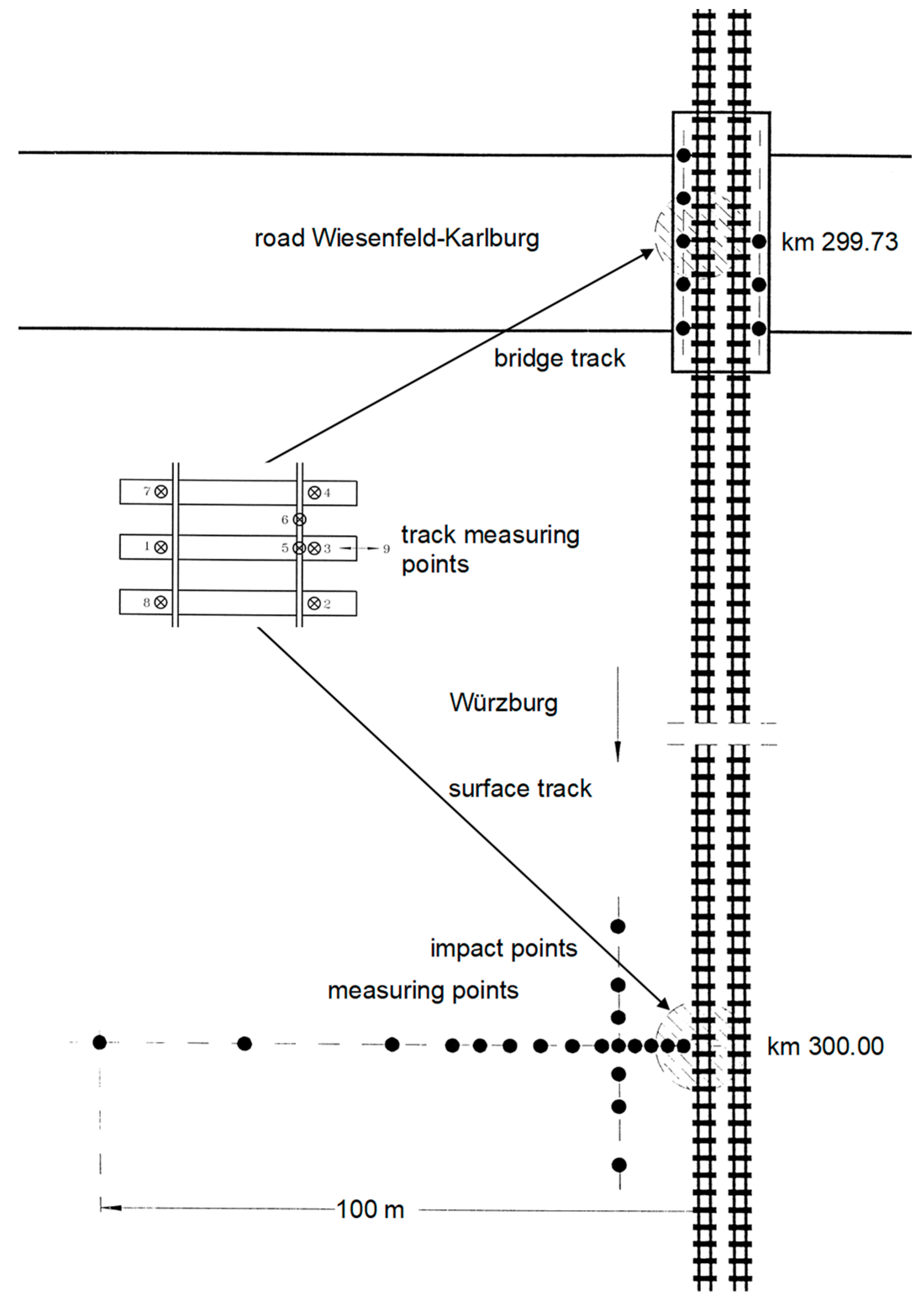
Simultaneous measurements of the vehicle, track, and ground vibrations have been performed in 1994 on a 3 km long test section of the high-speed line near Würzburg [
1]. The test train consisted of a locomotive E113, two carriages, a measuring car, two carriages, and a locomotive E111. The axle load of the measuring car is 100 kN, its wheelset mass is 1500 kg. Measurements have been performed simultaneously at three different track situations: at a surface line and a bridge with a ballasted track and at a tunnel with a slab track. The ballast track at the surface and the bridge consists of UIC60 rails on B60W sleepers with ZW687a rail pads. The high-speed track was in a good condition (low irregularities).
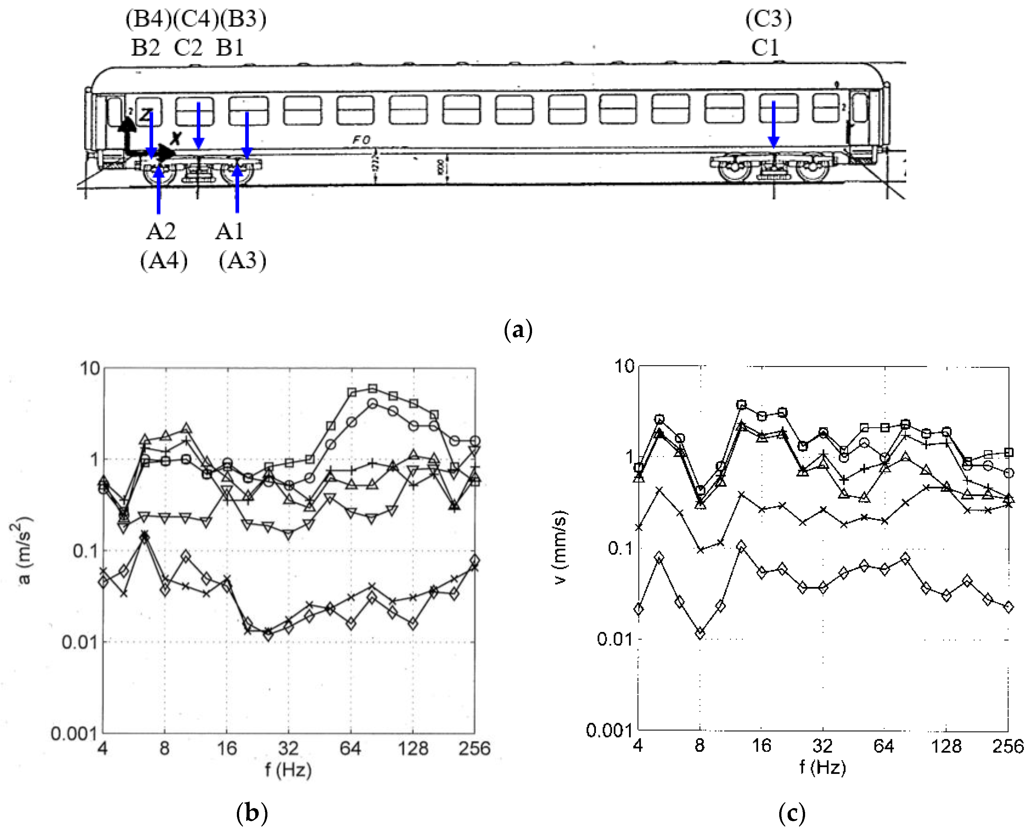
The vibration of the vehicle (the third carriage of the train) has been measured with accelerometers at 12 vertical and 3 horizontal measuring points (
Figure 1a). Four accelerometers (A1 to A4) have been mounted on the axle boxes of two wheelsets, and four accelerometers (B1 to B4) have been mounted at the corresponding points of the bogie frame. Four accelerometers (C1 to C4) have been mounted at the car body above both bogies. At the bogie and car body points B2, B4, and C2 also have horizontal accelerations that have been measured. All measuring points are chosen symmetrically for the left and right side of the passenger car [
37]. The vibrations of the three different tracks have been measured with geophones (velocity transducers) at 3 × 8 measuring points (2 rail and 6 sleeper points). The vibration of the ground has been measured with 14 geophones in a measuring line up to 100 m distance from the track, as per the layout of the measurements in
Figure 2.
The test train has run on the test section with the following train speeds
A subset of these measurements, the train passages at the surface line, are used in the present manuscript to be compared with theoretical analyses. These measurements have been recorded using a 72-channel measuring system with programmable filters (here used for anti-aliasing), sample and hold amplifiers, and a 16-bit AD converter running at 2 kHz sampling rate. The measurements have been evaluated uniquely for a 2-s time record around the passage of the measuring car over the instrumented track section. The one-third octave band spectra in
Section 3 are calculated from the corresponding Fourier spectra.
In addition to the train passages, each system has been characterized by impulse measurements (hammer impacts), the rigid and flexible modes of the railway vehicle, the flexible modes of the wheelset, the natural modes of the bridge, the receptances of the three tracks, and the transfer mobilities of the soil. The modes of the car body have been measured for 92 degrees of freedom and the results are shown in
Section 4.2 together with the theoretical analysis. To assure that natural modes have been identified, an identifier function (phase resonance function) has been evaluated, as per the details in [
38]. The measurements of the wheelset modes will be shown in
Section 5 in comparison with the theoretical results.
3. Vehicle, Track, and Soil Vibrations Measured during Train Passages
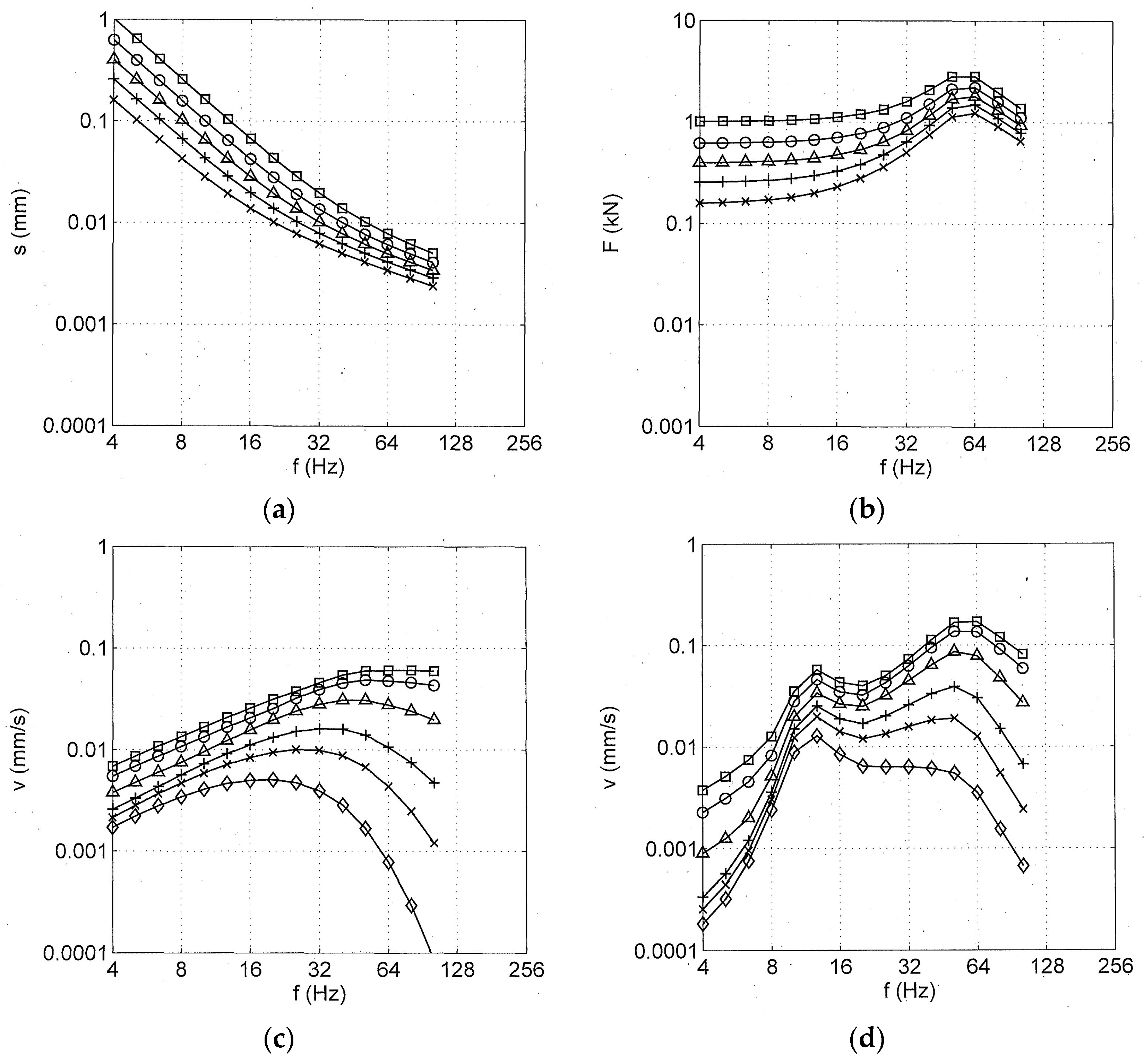
At first, the measured vehicle, track, and soil vibrations are presented and compared for the train passage with 160 km/h. The accelerations of the vehicle have been measured for the different vehicle components (
Figure 1a) and the corresponding accelerations are shown as one-third octave band spectra in
Figure 1b. The bogie accelerations are almost constant over the whole frequency range of 4 to 256 Hz with amplitudes of 0.5 to 1.0 m/s
2. The carriage has much lower amplitudes between 0.01 and 0.1 m/s
2 where the higher values are for frequencies below 20 Hz and the lower amplitudes are for higher frequencies. The highest accelerations have been measured for the wheelsets, which are up to 5 m/s
2 for frequencies between 50 and 160 Hz. At frequencies below 30 Hz, the wheelset accelerations are lower at about 1 m/s
2, all wheelset spectra are the same and the wheelset and bogie spectra are quite similar. Some raised amplitudes occur between 6 and 10 Hz where the bogie has twice the amplitude compared to the wheelset. The horizontal accelerations of the bogie are smaller with 20–30% of the vertical amplitudes. All these trends will be explained with the models and calculations in
Section 5.
Figure 1c shows the measurement results for the track, the one-third octave band spectra of the particle velocities of different track elements. These velocity spectra are almost constant over the whole frequency range and have values around 1 mm/s for the sleepers. The rail amplitudes are higher by a factor of 1.5 to 2 because of the elastic rail pads between sleeper and rail. The horizontal sleeper amplitudes are 10– 20% of the vertical sleeper amplitudes. These amplitudes are for a smooth curve of 5000 m radius and would be even smaller for a straight track. As a conclusion of the small horizontal amplitudes for the track, as well as for the vehicle (
Figure 1b), the horizontal vibrations are neglected in the present analysis and in the prediction scheme. Finally, the subsoil amplitudes are very small, by a factor of 30 smaller than the sleeper amplitudes. All these track vibrations have the same characteristics of the spectra. There is a strong minimum at 8 Hz and a weak minimum at 25 Hz; a maximum is found at 5–6 Hz and for 12–20 Hz. The three raised thirds of the octaves are not the same as those of the vehicle between 6 and 10 Hz. The characteristics of the track spectra are caused by the sequence of the passing axles [
38], which cannot be observed from the vehicle. Moreover, the track spectra up to 30 Hz are dominated by the passing static loads, and the response to the dynamic vehicle loads can only be observed at higher frequencies. It should be noted that at high frequencies, the left and right rails and sleeper ends have different spectra whereas they are the same for the low- and mid-frequency range. This trend can also be observed for the right and left axle-box accelerations in
Figure 1b, and it will be explained by the different vibration modes of the wheelset at high frequencies.
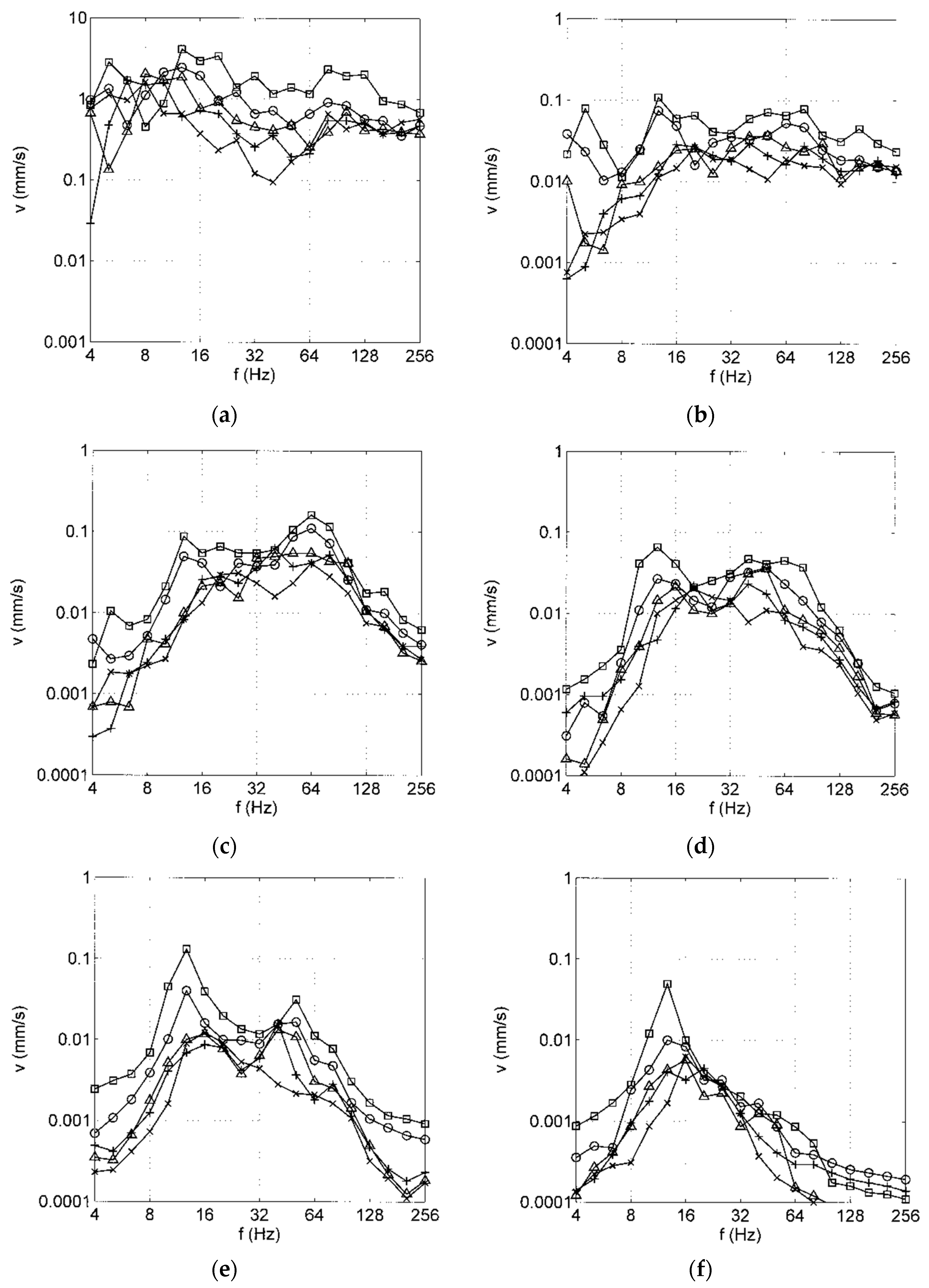
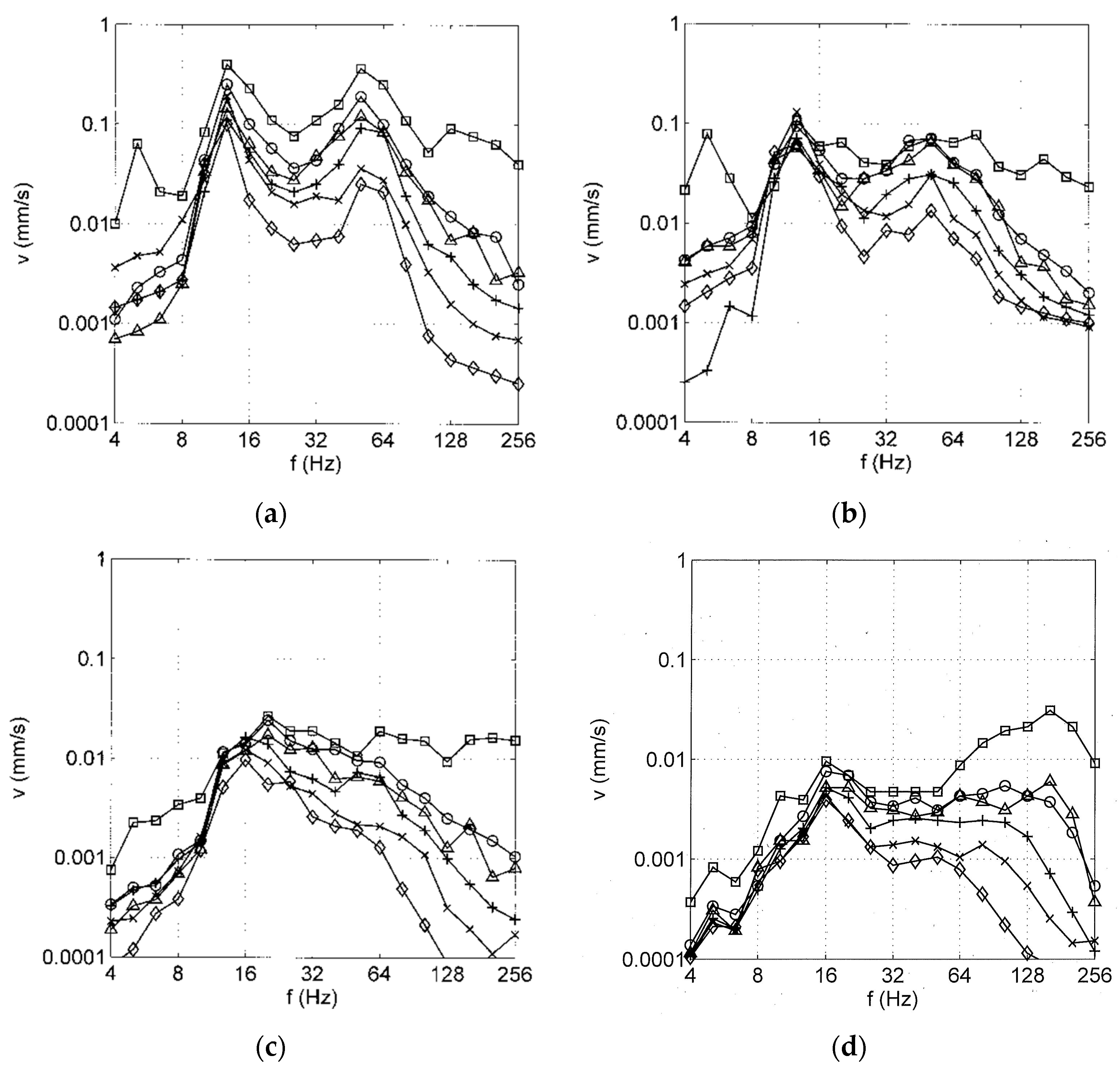
The ground vibrations measured for the train speed of 160 km/h are presented as the one-third octave band spectra of the particle velocities at distances from 2.5 to 50 m (
Figure 3a,b). The main amplitudes can be found between 10 and 80 Hz, whereas frequencies below 10 Hz and above 80 Hz are strongly reduced. Moreover, a strong attenuation with distance is observed in these frequency ranges. At low frequencies, there is an abrupt reduction from 2.5 m to 5 m distance. At high frequencies, there is a more regular reduction of two decades up to a distance of 50 m. The weakest attenuation of half a decade for 50 m can be found in the mid-frequency range at 10–16 Hz. These filter and attenuation effects lead to a dominant frequency of 12 or 16 Hz in the far field. This frequency peak (and a second weaker peak at 50–64 Hz) are even stronger for the passage of the locomotive in
Figure 3a. The same shape of the spectra can also be found for lower train speeds of 63 and 25 km/h with lower amplitudes (
Figure 3c,d).
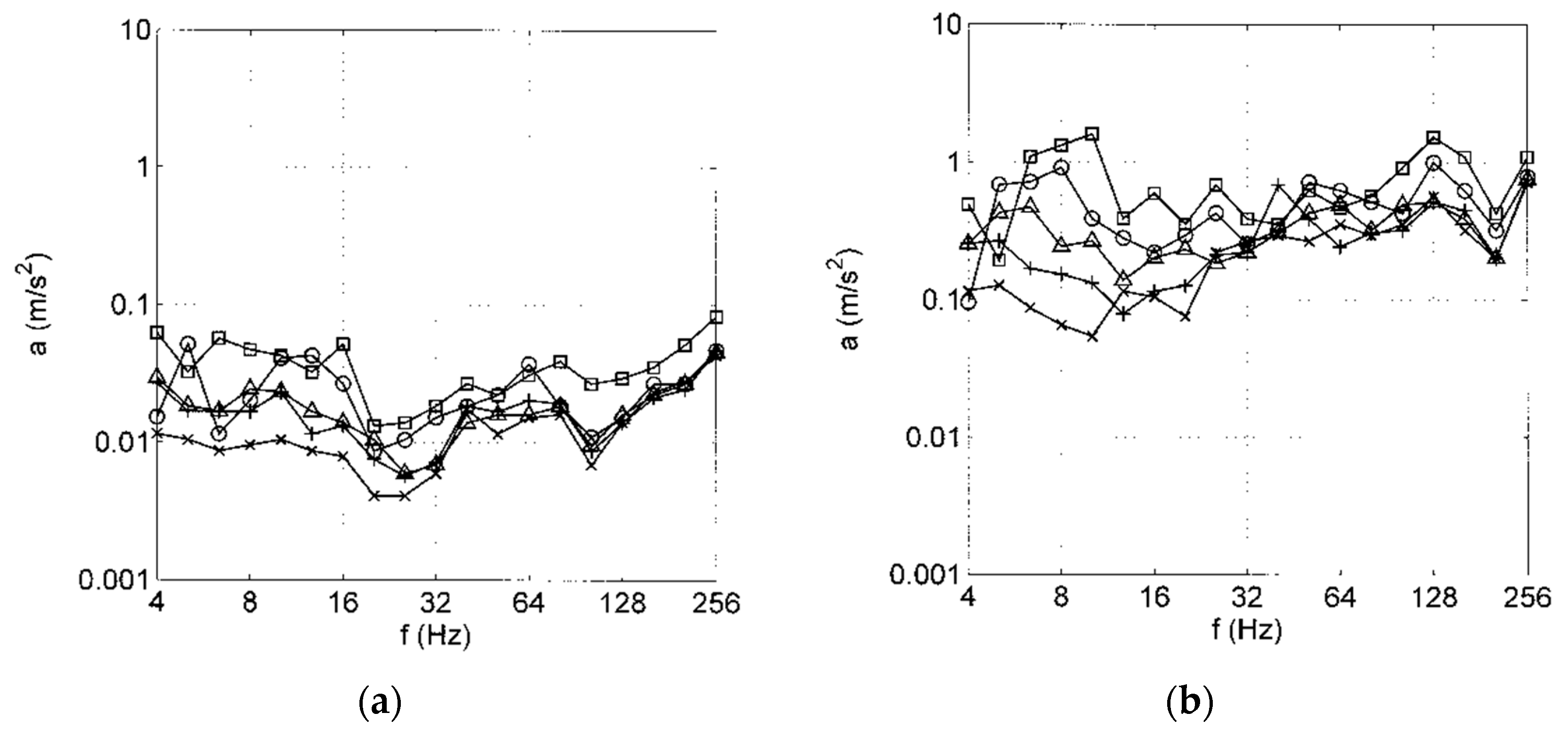
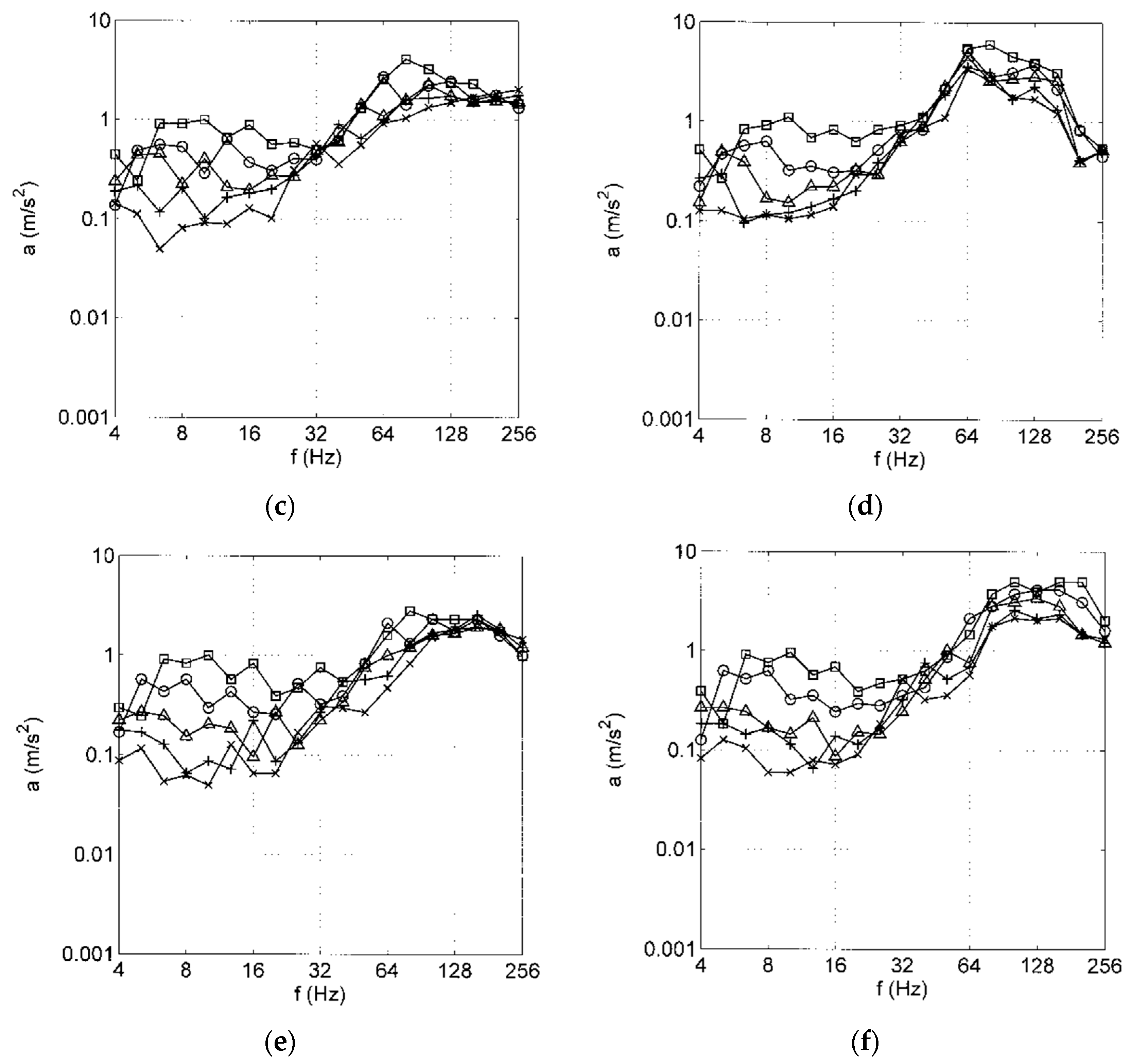
The Influence of the train speed is further analysed with
Figure 4 and
Figure 5. The car body (
Figure 4a) has low amplitudes, which increase with the train speed while the shape of the spectra with a typical decrease at 20 Hz remains constant. The bogie (
Figure 4b) shows a similar increase of amplitudes with train speed mainly at low frequencies. For the wheelsets in
Figure 4c–f, the accelerations increase clearly with the train speed as
a~
vT2, which means that the displacements of the wheels are speed independent in this low- and mid-frequency range and directly represent the track and vehicle irregularities. The somewhat greater high-frequency amplitudes increase less strongly with the train speed. The low- and mid-frequency wheelset and bogie spectra are shifted to higher frequencies with increasing train speed. This can be seen for the component between 6 and 10 Hz and for the maxima at 16 and 32 Hz for 160 km/h, which are the first and second out-of-roundness of the wheels [
39]. At high frequencies, a specific maximum is shifted from 32 to 40, 50, 64, and 80 Hz (most clearly in
Figure 4c), which is the frequency due to the distance of the sleepers [
40]. The wheel A2 (
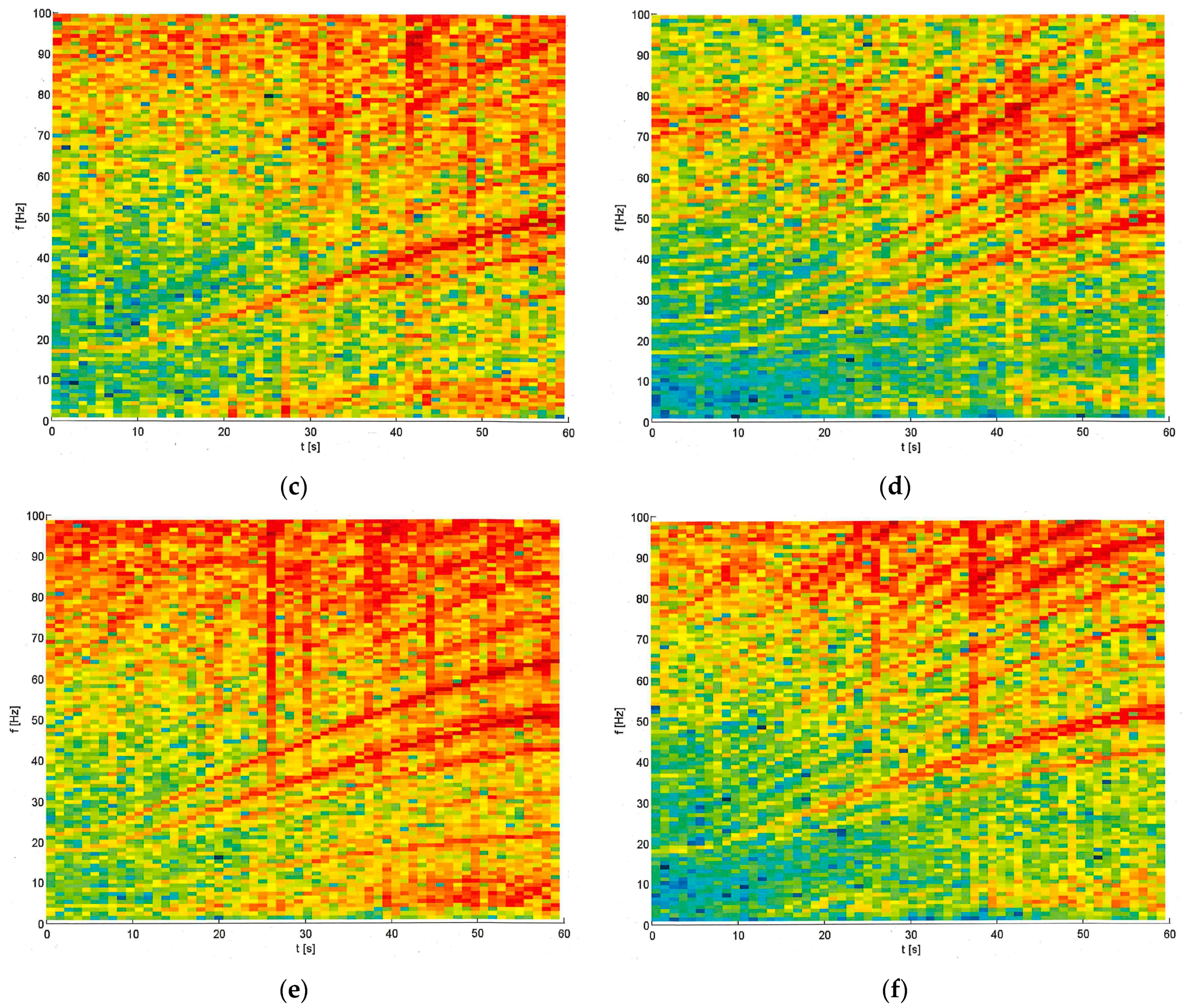
Figure 4d) shows a fixed dominant frequency of 64 Hz, which hides the sleeper–distance maxima. Another fixed frequency, though weak, can be found at around 100 Hz, which could also be attributed to a vehicle or vehicle–track eigenfrequency. The specific speed-dependent or speed-independent frequencies are also analysed with narrow-band spectra in
Appendix A, confirming the observations in the one-third octave band spectra with greater details.
The influence of the train speed on the track and ground vibrations at different distances is presented in
Figure 5. There is a general increase of velocity amplitudes with train speed, most clearly for the track (
Figure 5a). The maximum rail amplitudes increase quite regularly as
vmax~
vT, which means that the rail displacements are almost the same for all train speeds. This maximum, comprising three thirds of octaves (10 to 16 Hz for 160 km/h), is also regularly shifted with train speed. Such a regular behaviour cannot be found for the soil measuring points. A frequency shift can be seen in
Figure 5b for the lowest frequency of 4 and 5 Hz at 125 and 160 km/h, which belongs to the quasi-static response [
38]. Another frequency shift can be followed at 5 m distance (
Figure 5c) for the sleeper–distance frequency of 32 to 80 Hz. The more dominant maxima, however, are at 12 and 64 Hz. The high-frequency maximum at around 64 Hz loses its importance for the farer measuring points, and only the mid-frequency maximum of 12 Hz is left over at 100 m (
Figure 5f). For this maximum, the clearest increase of amplitude can be observed for 125 and 160 km/h, where the amplitudes are up to 10 times higher than those of the lower speeds. The two speed-independent peak frequencies seem to be related to vehicle or soil resonances. Moreover, the specific shape of the spectra of different distances are strongly determined by the transfer function of the soil, which is so dominant that other vehicle and track characteristics are mostly hidden.
The following similarities can be observed between the vehicle, track, and soil vibrations. The low-frequency high-speed component can be found in the track and the near-field soil spectra, and it has been identified as the quasi-static response in [
39]. The high-frequency maximum around 64 Hz can be found in the wheelset and in the mid-field ground vibrations. The most important maximum is around 12 Hz, which is dominant at the far field and has especially high amplitudes for the highest speeds and can also be found at the track at high speeds, but it is shifted to lower frequencies for lower train speeds. The layering of the soil at the measuring site yields an eigenfrequency at 12 Hz, but the resonance amplification is usually not so high. Finally, vehicle eigenfrequencies also occur in this mid-frequency range; for example, the bogie amplitudes are amplified at a slightly lower frequency range. The purpose of the following sections are to analyse possible vehicle resonances in the mid-frequency range around 12 Hz (below 40 Hz,
Section 4) as well as in the high-frequency range around 64 Hz (above 40 Hz,
Section 5) and their effects on the excitation forces of the ground vibrations.
4. Analyses of the Vehicle Dynamics at Frequencies below 40 Hz
The following sections analyse the influence of rigid bogie modes, flexible carriage modes, and flexible wheelset modes. The influence of the track has been analysed in detail by three-dimensional finite-element boundary-element models in [
29]. The track stiffness has no influence on the vehicle–track interaction at low and mid frequencies, such as at the rigid bogie and the flexible carriage modes, which therefore are discussed for a rigid track. At higher frequencies, the compliance of the track is important, and it is included as a soil-dependent spring stiffness in the analysis of the flexible wheelset in
Section 5. All analyses have been done by simple two- and three-degree-of-freedom systems, which could be introduced in the prediction software if necessary.
4.1. Rigid Body Modes of the Railway Vehicle at Frequencies below 40 Hz
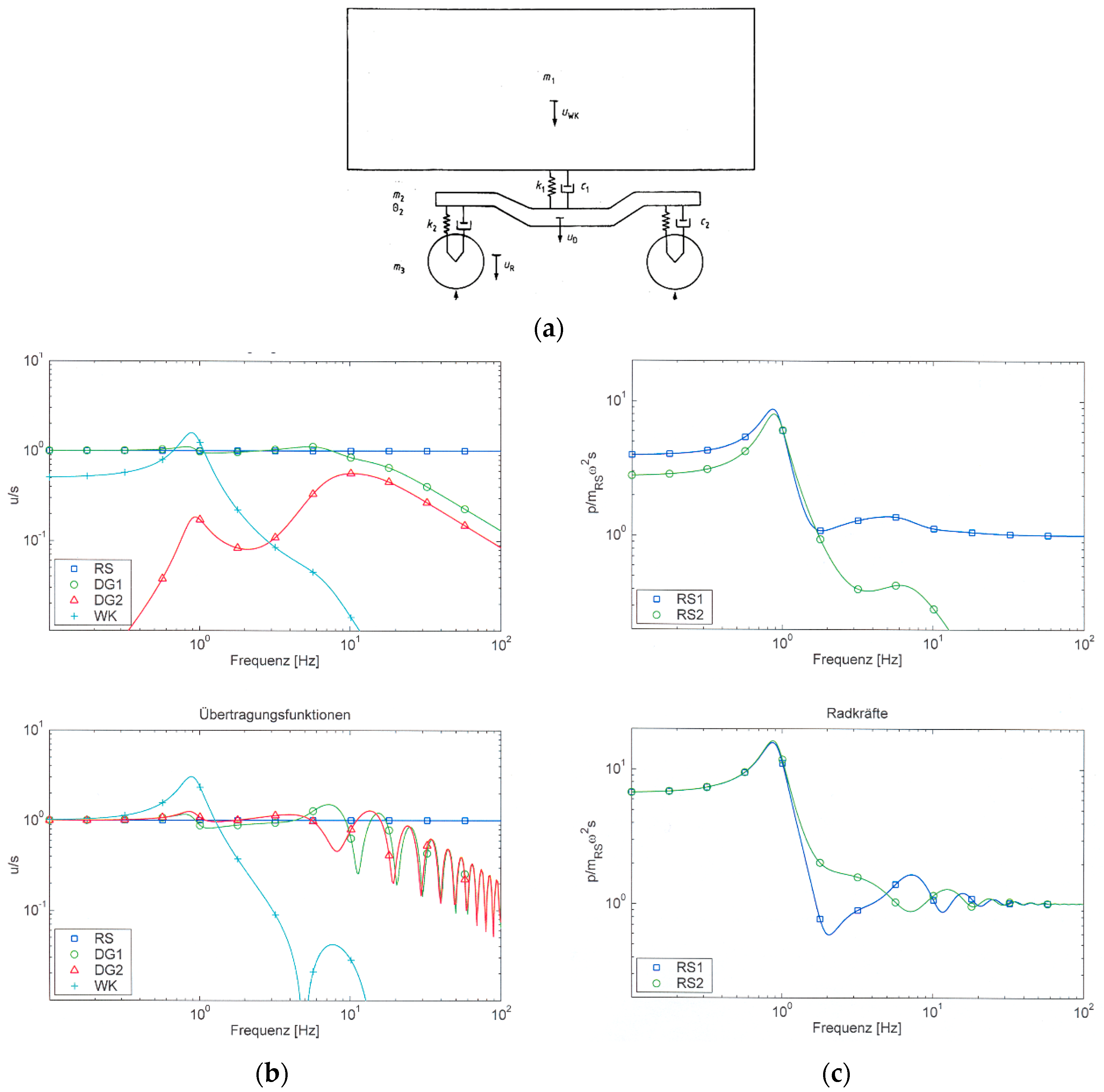
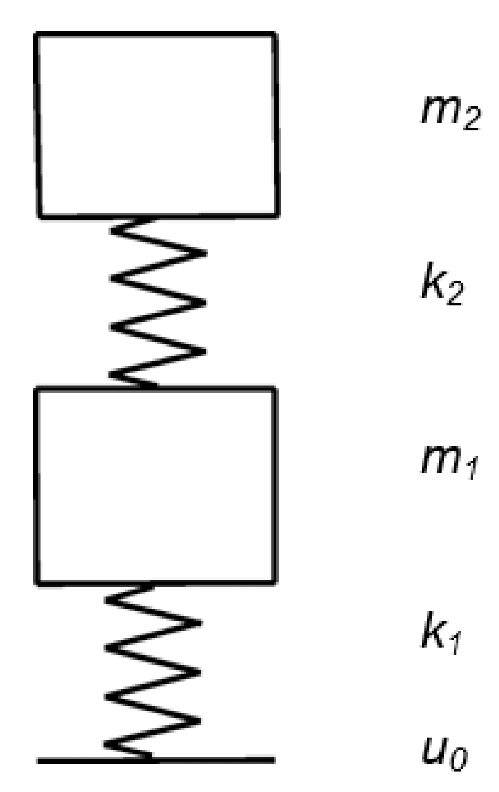
The rigid vehicle model of
Figure 6a is considered, which consists of two wheelset masses of 1700 kg (1550 kg), a bogie frame of mass 2800 kg (2500 kg), and the mass of half a car body of 16,500 kg (14,500 kg). The complete set of parameters of the ICExperimental mid car including the primary and secondary suspension can be found in [
40], together with the measured ground vibration. The values in brackets are for the passenger car of the measuring campaign [
1], for which similar results have been found. The parameters can be used to get the vertical and the pitching eigenfrequencies of the bogie
The eigenfrequency of the car body can clearly be found at about 1 Hz as a resonance of the car body response, shown at the top of
Figure 6b. The bogie resonances show little resonance amplification, the excited bogie part 1 shows the vertical eigenfrequency, the second not-excited bogie part has its maximum near the pitching eigenfrequency.
The displacements which are shown at the top of
Figure 6b are calculated for a harmonic excitation
s of one wheelset. At the very low frequencies below 1 Hz, the excited bogie part B1 exactly follows the excitation while bogie part B2 is almost at rest. The car body follows with half of the one-sided excitation. With increasing frequencies, the different components of the vehicle decouple from the excited wheelset. At first, the car body is decoupled above its eigenfrequency of 1 Hz, then the bogie above its vertical eigenfrequency of 7 Hz or above its pitching eigenfrequency of 14 Hz. In case of a flexible track, there is also a wheelset–track eigenfrequency between 50 to 100 Hz, above which the wheelset decouples from the excitation, as seen in
Section 5. All of these trends can also be found in good agreement with the measurements in
Figure 1b and
Figure 4.
The one-sided excitation includes the symmetric and antimetric excitation of the bogie uniquely for all frequencies. Under real conditions, shown at the bottom of
Figure 6b, both wheelsets of a bogie are excited by the same track irregularities, which have a certain time delay or a phase delay that increases linearly with frequency and is inverse to the train speed
vTFor the wheelset distance lA = 2.8 m and the train speed vT = 100 km/h, the phase delay is π at f = 5 Hz (anti-phase excitation), 2π at 10 Hz (in-phase excitation). More antimetric excitations follow at 15, 25, 35, … Hz. At low frequencies, the phase is close to zero. For this in-phase excitation, all masses follow the excitation (u/s = 1). Between 1 and 5 Hz, the second bogie part has higher amplitudes than the first bogie part. The antimetric excitation at 5 Hz yields identical amplitudes of both bogie parts and zero displacements of the car body due to the pure rotation of the bogie frame. For higher frequencies, there are regular variations of the bogie displacements due to the regular sequence of the symmetric and antimetric excitation. As the vertical mode has a lower eigenfrequency, it is more strongly reduced than the rotational mode at higher frequencies. Therefore, maxima are found for antimetric excitation and minima for symmetric excitation.
Corresponding results for the wheel–rail forces are shown in
Figure 6c. For the one-sided excitation (
Figure 6c top) the wheel–rail force of the excited first wheelset is higher than for the unexcited second wheelset. The difference is the inertial force of a wheelset. At frequencies below 1 Hz, the force is the inertial force of the whole (quarter) vehicle. At high frequencies, the force at the excited wheelset is the inertial force of this wheelset, while the force of the unexcited wheel tends to zero.
The bottom of
Figure 6c shows the wheel–track forces for the realistic two-wheelset excitation with phase delay. For this realistic case, both wheelset forces tend to the inertial force of the wheelset for frequencies higher than 20 Hz. At very low frequencies below 1 Hz, the forces are the inertial forces of the whole vehicle, which are approximately seven times higher than the wheelset forces. The decrease of the forces follows immediately after the car body resonance, and the forces are close to the wheelset forces in the intermediate range of 5 to 20 Hz. For these frequencies, there are some differences between the first and the second wheelset and variations with frequency, which decrease rapidly with increasing frequency. It is observed that the force of the first wheelset is smaller than that of the second wheelset in the intermediate frequency range of 1 to 5 Hz. The possible amplification is not stronger than two, which would correspond to the mass of the wheelsets and the bogie frame. The restricted influence of the bogie resonances is due to the small inertia of the bogie frame and the strong damping of the primary suspension for the passenger cars considered here, and this conclusion was checked for other passenger cars and other train speeds.
The special bogie effects can also be found in the vehicle measurements (
Figure 1b and
Figure 4b) where a certain track irregularity is amplified by a factor of 1.5–2 for the bogie at 5–8 Hz (
v = 125 km/h) and at 6–10 Hz (
v = 160 km/h). These frequencies are not the frequencies of strong ground vibration, thus from the experimental view, accelerations of the bogie frame are not expected as a significant excitation of ground vibration.
4.2. Elastic Modes of the Car Body
A modal analysis of the measuring car, a typical passenger car of the German Railway, has been performed in a workshop in Würzburg [
1,
41]. The passenger car has been excited by hammer impacts so that the mode shapes could be established for 92 degrees of freedoms, 44 of the car body, 2 × 20 of the bogies, and 4 × 2 of the wheelsets. Besides rigid body modes in the range of 1.2 to 4 Hz, clearly separated elastic modes of the car body have been identified in
Figure 7. The first bending mode is at 9 Hz, the lateral bending mode is at 11 Hz; the first torsional mode is at 14 Hz, and the second bending mode is at 18 Hz. Note that the two vertical eigenfrequencies have also been found during the test runs, as seen in
Figure A1a in
Appendix A. All of these elastic modes of the car body are in the frequency range of strong ground motion. The effect of these elastic modes on the excitation of ground vibration is analysed by a simple beam model on the support springs and dampers of the secondary suspension.
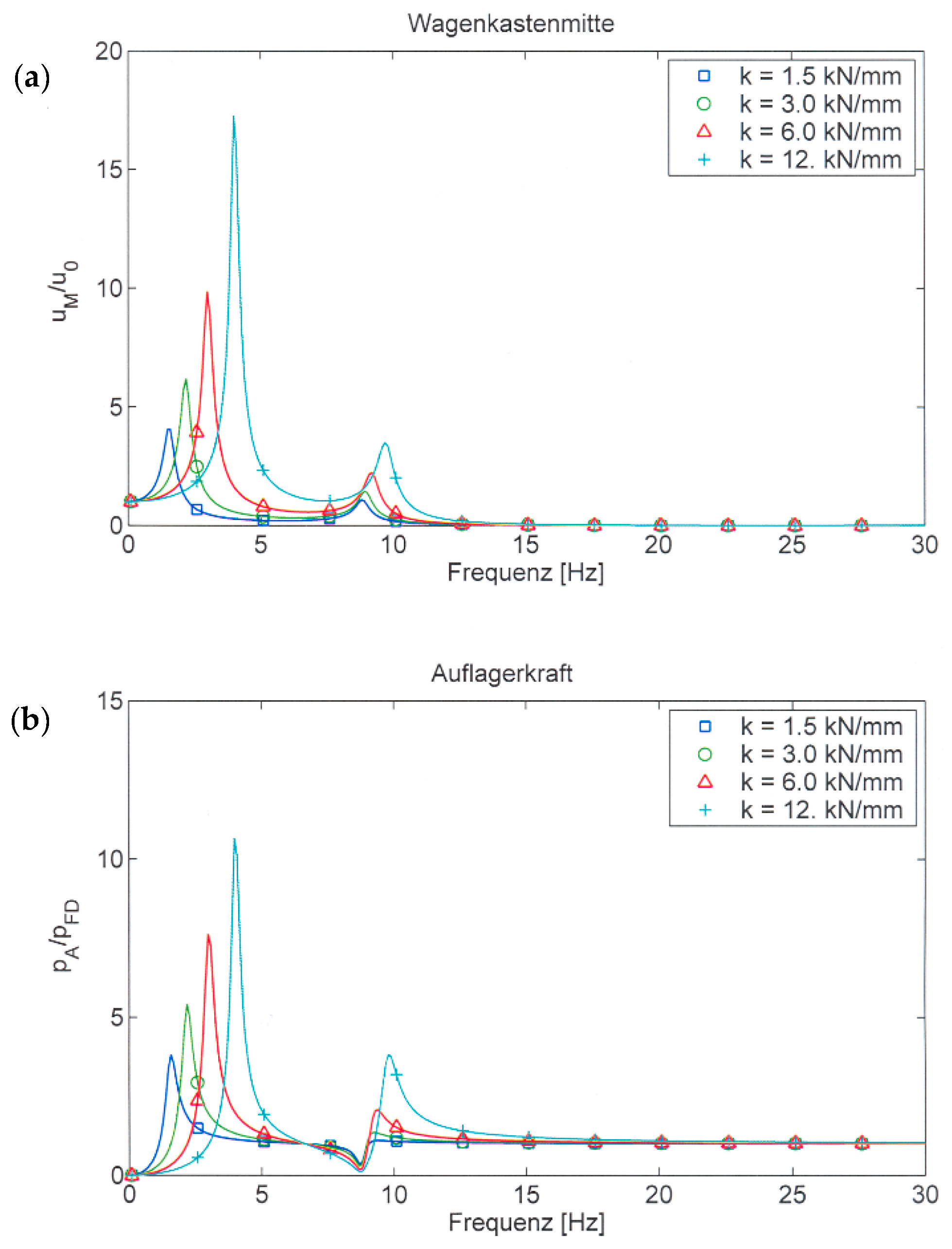
The elastic support yields the rigid mode of the car body, which is at 1–5 Hz depending on the support stiffness (
Figure 8a). A second maximum is found at 9 Hz for the displacement of the middle of the car, which is due to the first bending mode. The forces at the support (
Figure 8b) show the rigid resonance below 5 Hz, but a minimum at the elastic eigenfrequency at 9 Hz. A maximum follows immediately, which has no considerable amplification for realistic support spring stiffnesses.
These results can be generalised as follows: The elastic modes of the car body are almost the modes of the free and unsupported car body and occur at almost the free eigenfrequency. For the free modes, all inertial forces are balanced and no support forces appear. As the frequencies of the supported and unsupported modes are close together, the support forces are small at these eigenfrequencies. Under normal soft and medium support stiffnesses (secondary suspensions), the support forces have no important amplification in the “resonance region”.
Therefore, it can be concluded that the elastic modes of the car body, as well as the rigid bogie modes of
Section 4.1, are not a reason for the pronounced ground vibration. Consequently, the forces below 40 Hz can be approximated by the rigid wheelset mass. Moreover, in this low- and mid-frequency range, the irregularities
s of the wheel and track can be calculated directly from the axle-box accelerations
a as
s~
a/
ω2 without any influence of the vehicle model.
5. Wheelset–Track Analysis at Frequencies above 40 Hz
A typical wheelset of the passenger car, which has also been measured during the campaign, has been calculated as a finite-element model for different support conditions [
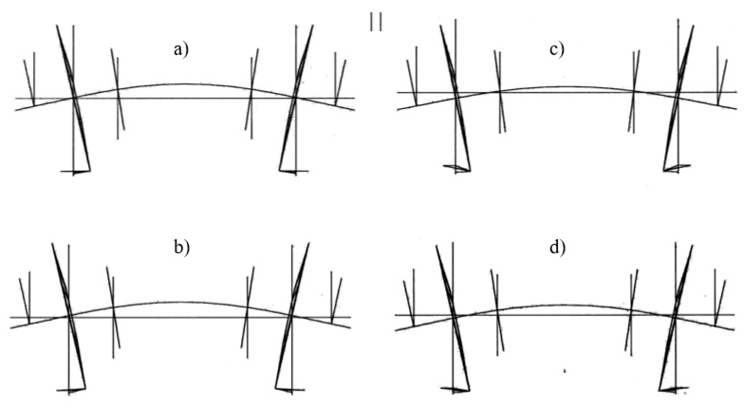
42]. The most important eigenfrequencies of the wheelset are shown in
Figure 9. The wheelset on a medium stiff support
k = 5 × 10
8 N/m has an in-phase eigenfrequency at
f1 = 62.7 Hz and an anti-phase eigenfrequency at
f2 = 90.3 Hz, where the wheels and the mid-axle are in anti-phase. In addition to these coupled modes, there is the rolling mode at 84.7 Hz and the horizontal bending mode at 70.9 Hz, which is also the vertical free bending eigenfrequency of the wheelset.
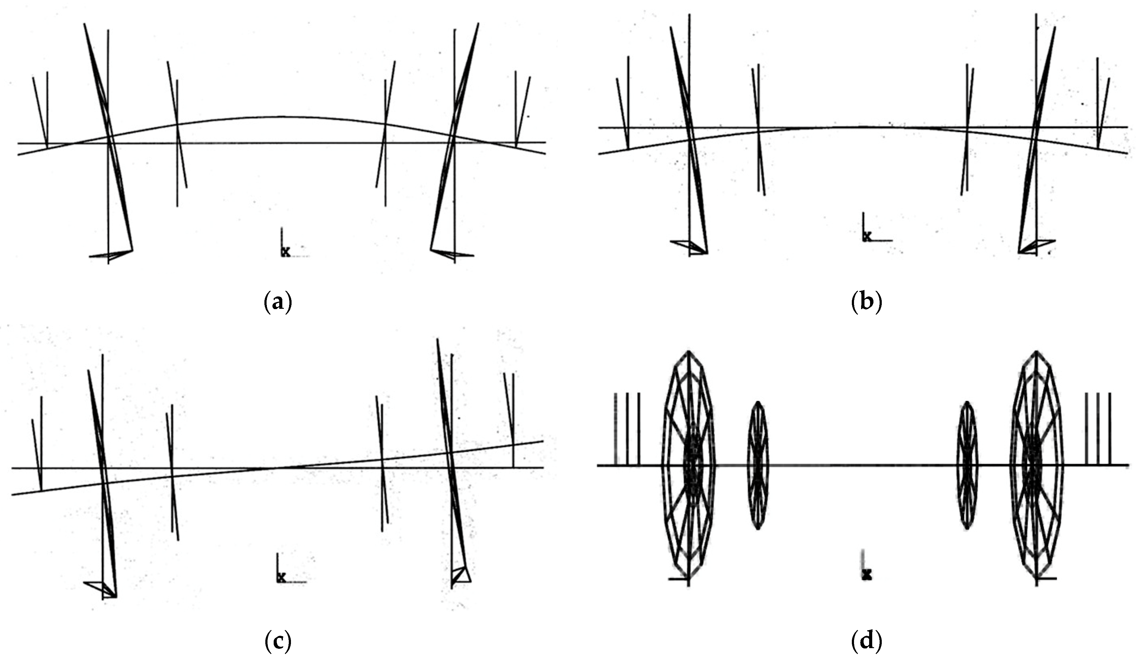
The vertical modes vary with the support stiffness
k. If the support is very stiff (
k = 50 × 10
8 N/m,
Figure 10a), the eigenfrequency
f = 66.8 Hz approaches the eigenfrequency of the rigidly supported wheelset. If the support is very soft (
k = 0.5 × 10
8 N/m,
Figure 10d), the eigenfrequency
f = 71.8 Hz tends to the eigenfrequency of the free wheelset. For realistic stiffness parameters, the eigenfrequencies are not so far from these two limit cases. For a medium stiff
k = 10 × 10
8 N/m, the eigenfrequency
f = 65.4 Hz is somewhat above the rigidly supported eigenfrequency (
Figure 10b), and for a soft support with
k = 2.5 × 10
8 N/m, the eigenfrequency
f = 77.3 Hz is somewhat above the free eigenfrequency (
Figure 10c). These somewhat contradictory results with a frequency jump between
k = 2.5 and 10 × 10
8 N/m will be further explained at the end of this section.
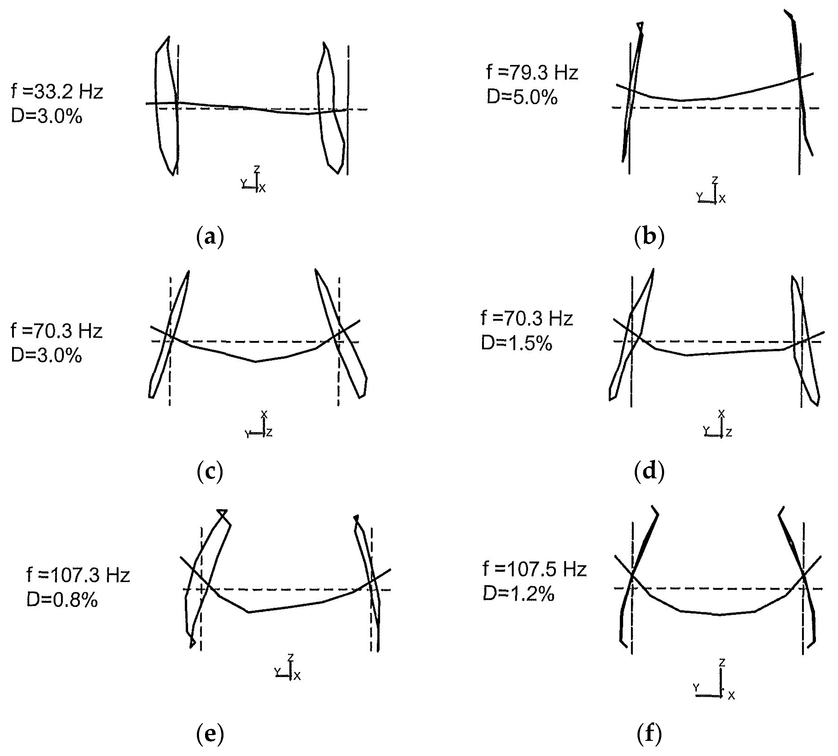
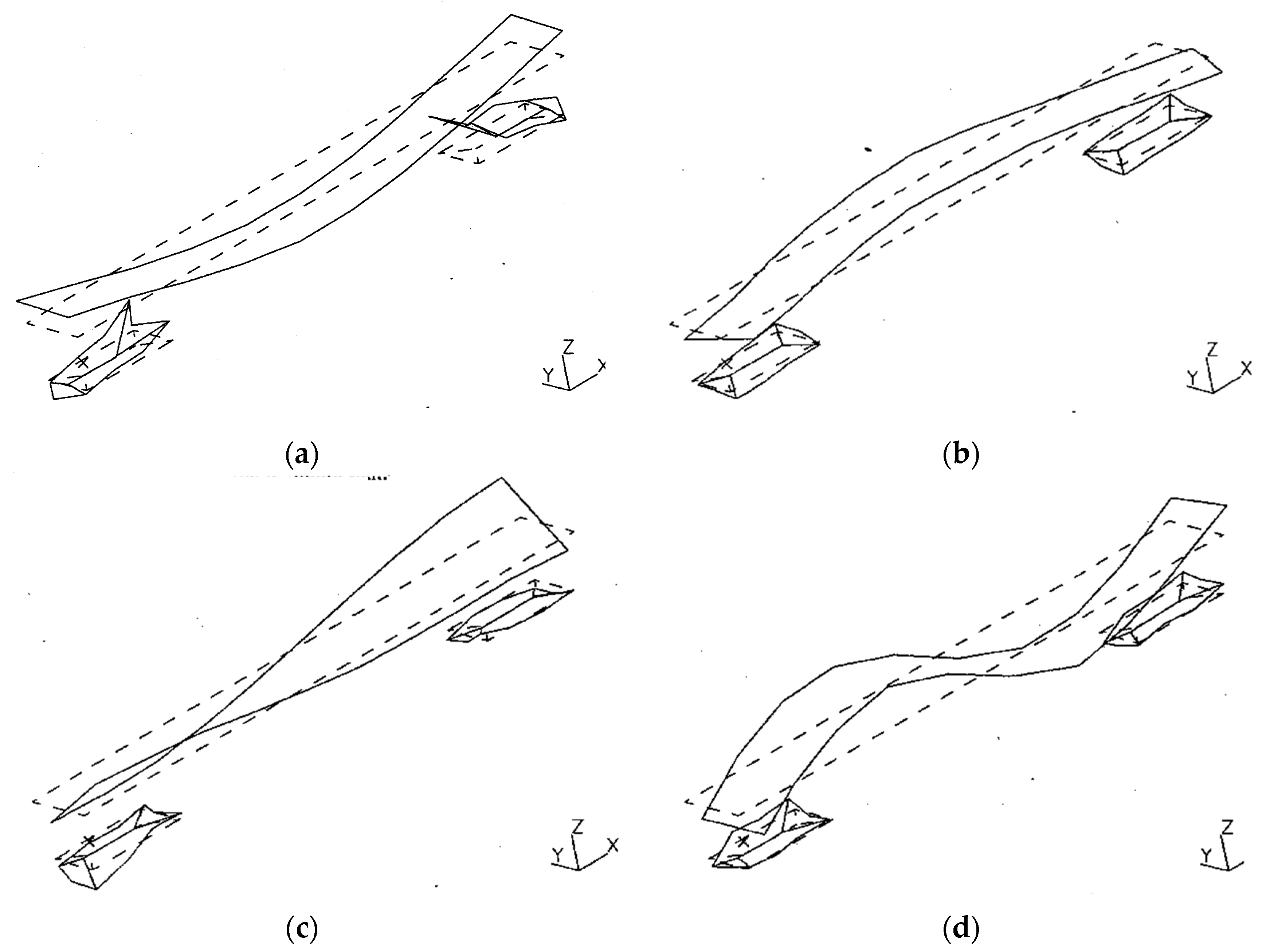
The calculated eigenfrequencies and mode shapes are confronted with an experimental modal analysis of a similar wheelset in a workshop [
42], as seen in
Figure 11. The wheelset was instrumented with 12 × 2 × 3 geophones around the two wheels and 7 × 3 geophones along the axle (all in three directions) and excited by a hammer vertically in the mid of the axle (shifted by 0.3 m) and horizontally at the upper end of one of the wheels (shifted by 30°). The horizontal excitation yields the mainly horizontal mode at 33.2 Hz, and the vertical excitation yields the mainly vertical mode at 79.3 Hz. The latter includes an anti-phase bending component. The free bending mode (in horizontal direction) has been found at 70.3 Hz for both excitations. The restrained bending mode (in vertical direction) lies at 107.5 Hz for both excitations. This eigenfrequency is higher than in the running train and in the calculation because of the stronger horizontal fixation at the contact point. The main conclusion of the comparison is the confirmation that the free bending mode is at approximately 70 Hz, and that the two coupled vertical and bending modes are close together.
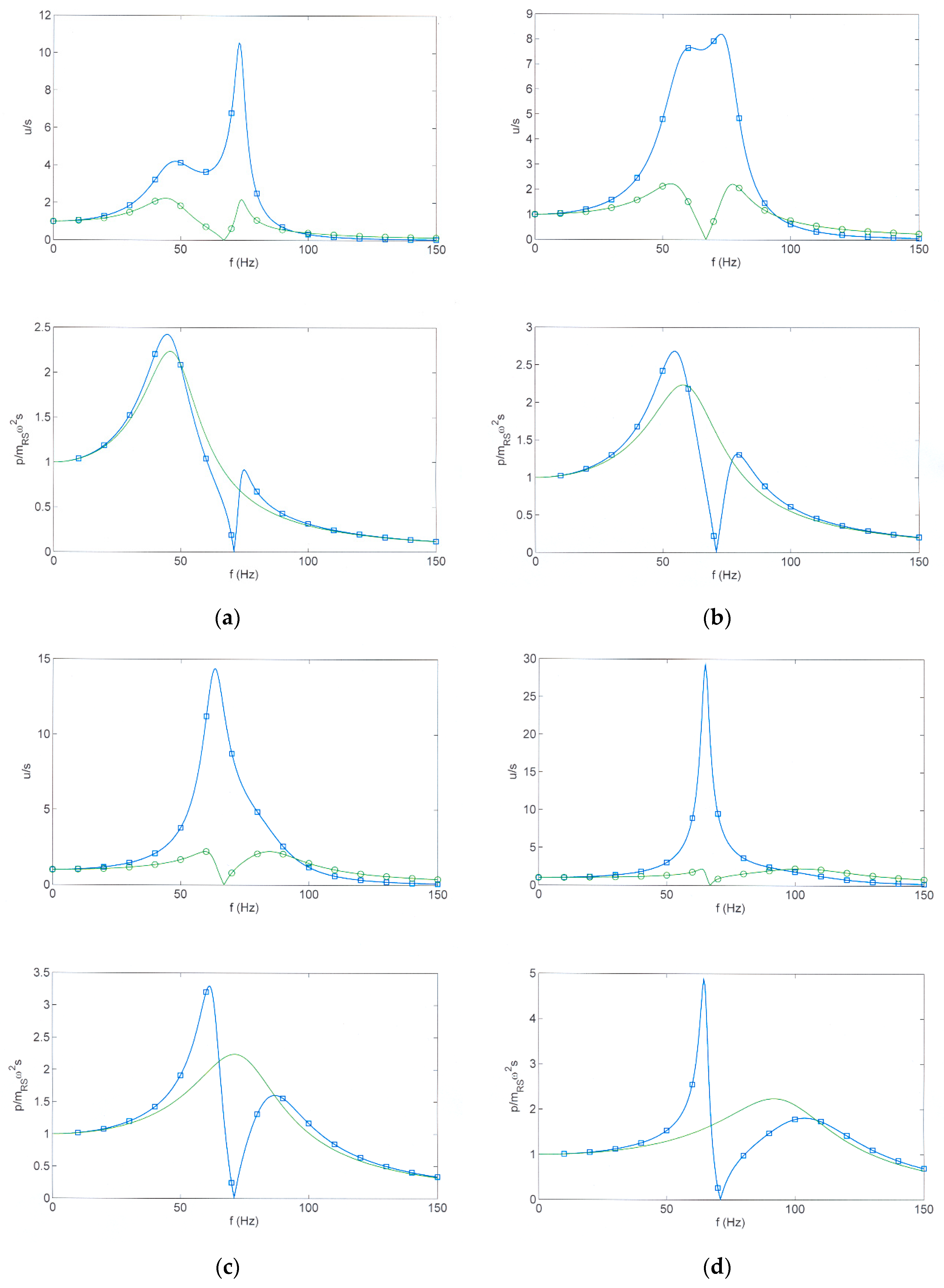
The frequency-dependent wheel and axle displacements are investigated by a simple two-mass model which is fitted to the known eigenfrequencies. It is given in full mathematical detail in
Appendix B for possible inclusion in a fast prediction software. The results of the simple model are, in general, similar to the results of a more complex and detailed finite element model in [
43]. In
Figure 12a–d (top), the two vertical resonances of the wheelset can be found, but the amplifications are different for wheel and axle and vary with the support stiffness. The highest amplification is for the axle mass, whereas the wheel mass has a smaller resonance and even a zero at the eigenfrequency of the rigidly bounded wheelset.
The dynamic support forces (
Figure 12a–d, bottom) also have a characteristic zero, which is at the eigenfrequency of the free wheelset. The first resonance is always stronger than the second resonance. The maximum amplification increases clearly with the stiffness of the support. Above the wheelset–track resonance, the force decreases compared to the inertial force of the wheelset. This is of importance for high-frequency excitations such as the sleeper–distance excitation for which the wheel–rail force increases according to
only for low train speeds and remains constant for high train speeds.
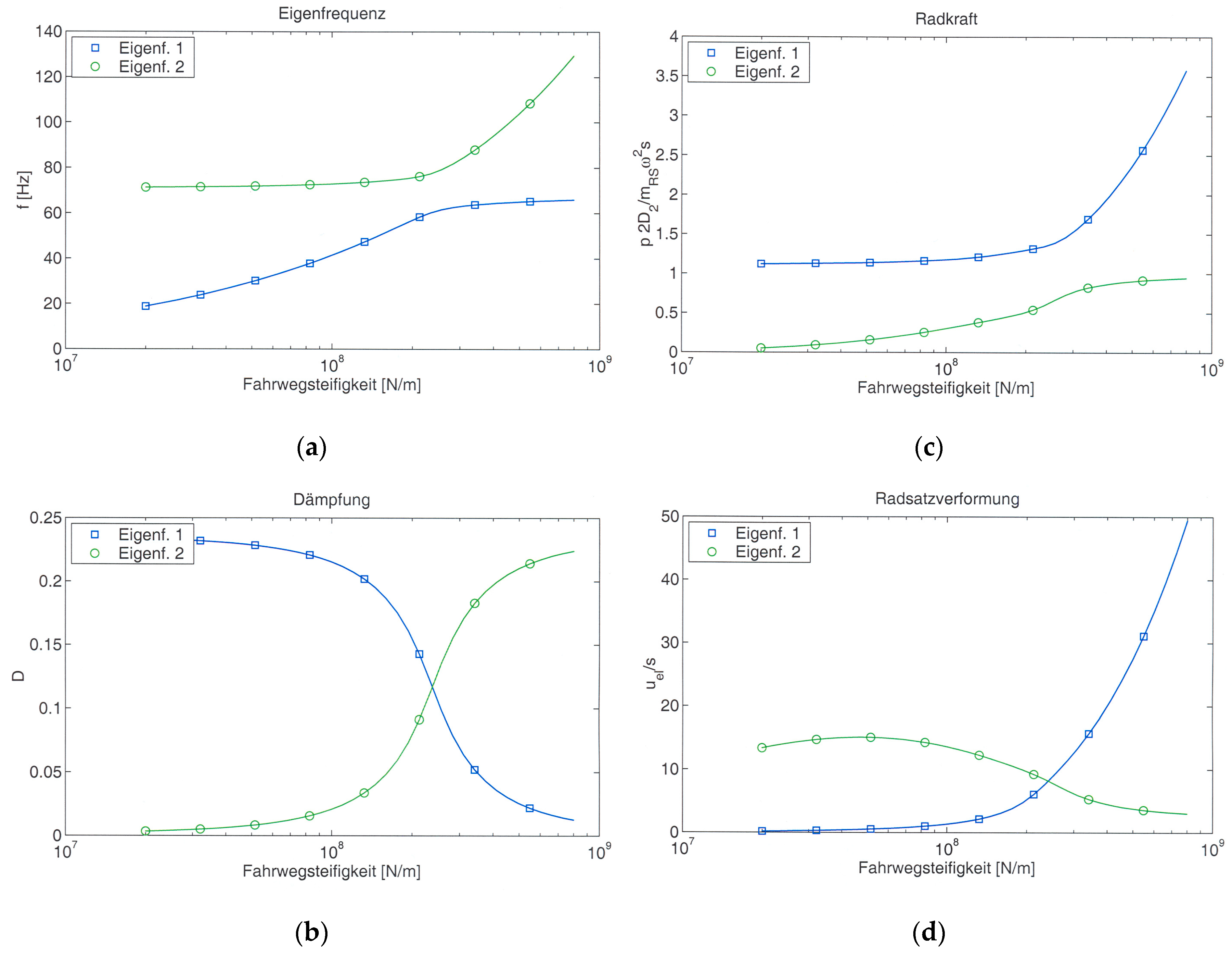
The variation of the response with the support stiffness is further demonstrated in
Figure 13. The resonance frequencies show two crossing asymptotes (
Figure 13a). One asymptote is the constant elastic eigenfrequency of the wheelset, the other asymptote is the rigid body eigenfrequency (the wheelset–track eigenfrequency), which increases with the support stiffness. Around the crossing of the asymptotes, the curves deviate from these asymptotes and the two eigenfrequencies change their role. The elastic eigenfrequency jumps from the upper curve to the lower curve and from the higher value of the free eigenfrequency to the lower value of the rigidly supported eigenfrequency.
The same things can be observed for the modal damping in
Figure 13b. For low support stiffnesses, the low rigid body resonance has the strong support damping of
D ≈ 0.25, and the higher elastic eigenfrequency has the low wheelset damping of
D = 0.001. For high support stiffnesses, the eigenfrequencies have changed their position but kept their characteristic damping. The damping curves meet in the medium stiffness range and both eigenfrequencies have a medium damping of
D ≈ 0.12.
The effect of the support stiffness on the maximum dynamic loads on the track is shown in
Figure 13c. The resonance force is compared with the resonance force of a rigid wheelset. This “rigid” resonance amplitude occurs for soft support stiffnesses and for the first eigenfrequency. The second eigenfrequency, which consists of an anti-phase vibration, always has a smaller resonance force. For low support stiffnesses, the second mode is the almost free bending mode of the wheelset with very small support forces. For high support stiffnesses, the support mode is the second mode with support forces that are a little smaller than the “rigid” resonance forces. The elastic mode is then the first mode at nearly the fixed mode, and the resonance amplitude increases considerably with the increasing support stiffness. Similar effects can be read from the difference of the axle and wheel displacement (the elastic deformation) at resonance in
Figure 13d. Once again, an increase of the elastic effects is found for the stiff support condition. Some explicit formula for the coupling of a flexible system with a track or a general support stiffness are derived for a two-mass system in
Appendix B.
The conclusion for the excitation of ground vibration is that the flexibility of the wheelsets does not yield a considerable force increase on the track and ground. The only exceptions are very stiff support conditions where resonance amplifications of the force at the elastic eigenfrequency of the wheelset are possible. Note that the relevance of the elastic wheelset mode is further limited by the primary damping, which has not been included for simplicity. Usually, the most important mode of the wheelset is the vertical vehicle–track mode, which yields a resonance and a force reduction at higher frequencies, whereas the elastic and rocking wheelset modes can be measured at the axle boxes and have no effect on the ground vibration (see also [
13,
44]) and can be neglected in the prediction.
6. Prediction of Irregularities, Force Spectra, and Ground Vibrations
As a result of the analyses in
Section 4 and
Section 5, the effect of the irregularities on the dynamic forces and the ground vibrations can well be approximated by the model of a rigid wheelset. The irregularity amplitudes
s decreases with frequency as
s~
f −2 for frequencies below 40 Hz and
s~
f −0.75 for frequencies above 40 Hz according to [
40] (
Figure 14a). As the force transfer function due to the inertia of the vehicle (the wheelset) increases with frequency at the same time, the resulting force spectrum (
Figure 14b) is nearly constant with some increase around the vehicle–track resonance. Some similarities can be found between the predicted excitation forces in
Figure 14b and the measured wheelset acceleration in
Figure 4c–f. The present axle-box measurements confirm the general trend, the smooth almost constant force spectra with amplitudes of approximately 1 kN per axle and third of octave. This general trend has also been checked by many ground vibration measurements at different sites in [
40]. The forces at higher frequencies, however, would be overestimated by the axle-box accelerations according to the analysis in
Section 5.
The ground vibration for a train load with a constant force spectrum and for a homogeneous soil is shown in
Figure 14c. The low-frequency velocity amplitudes increase systematically with frequency; the high-frequency amplitudes decrease due to the material damping of the soil. Therefore, the mid-frequency range between 16 and 64 Hz is dominant and these trends are in satisfactory agreement with the measurements. The prediction can be improved by using the calculated force spectrum and the transfer functions of the layered soil at the measuring site (
Figure 14d). The layering of the soil yields an additional low-frequency cut-off, and the layer resonance at 12 to 16 Hz and the vehicle–track resonance at 50 to 64 Hz are now included. The even higher measured mid-frequency amplitudes for 160 km/h (
Figure 3j) have been attributed to a scattering effect of the moving static loads, as seen in the detailed analyses in [
45]. The whole simple, fast, and efficient prediction scheme is given with all details in [
46].


 , ☐ wheelset A1 and A2, +, △ vertical bogie part B1 and B2, ▽ horizontal bogie part B1,
  , ✕ car body part C1 and C2; (c) particle velocities of the track ☐,