Adaptive Driving Style Classification through Transfer Learning with Synthetic Oversampling

Abstract

Driving style classification does not only depend on objective measures such as vehicle speed or acceleration, but is also highly subjective as drivers come with their own definition. From our perspective, the successful implementation of driving style classification in real-world applications requires an adaptive approach that is tuned to each driver individually. Within this work, we propose a transfer learning framework for driving style classification in which we use a previously developed rule-based algorithm for the initialization of the neural network weights and train on limited data. Therefore, we applied various state-of-the-art machine learning methods to ensure robust training. First, we performed heuristic-based feature engineering to enhance generalized feature building in the first layer. We then calibrated our network to be able to use its output as a probabilistic metric and to only give predictions above a predefined neural network confidence. To increase the robustness of the transfer learning in early increments, we used a synthetic oversampling technique. We then performed a holistic hyperparameter optimization in the form of a random grid search, which incorporated the entire learning framework from pretraining to incremental adaption. The final algorithm was then evaluated based on the data of predefined synthetic drivers. Our results showed that, by integrating these various methods, high system-level performance and robustness were met with as little as three new training and validation data samples in each increment.

1. Introduction

The understanding of a driver’s mood, intention, awareness, or other factors through the analysis of various driving data from different sensors plays a major role in improving both the safety and user experience of modern vehicles. For example, with the help of such information, the human–machine interface can be adopted to better match the driver’s expectations and to relieve the driver from the driving task. In this context, information about the current driving style may be used to select the appropriate drive program, which changes the behavior of major human–machine interfaces such as the visual dashboard, the steering system, and the powertrain. However, different drivers perceive driving situations and classify their driving style differently. Thus, a general and objective definition cannot be given for this application. Rather, we need a subjective approach that considers each driver and adapts individually, forming a customized driving style classification.

Within this work, we used a pretrained neural network, which was based on a heuristic rule-based driving style classification algorithm, as a baseline. We then applied transfer learning to different (synthetic) drivers to tackle the challenge of limited data. This is because we aimed at improving the individual classification with the minimum data possible, which are sparse in real-world applications. To achieve successful training, we performed feature engineering based on domain knowledge, calibrated the neural network using temperature scaling, and use a synthetic oversampling approach to stabilize the training.

In Section 3, we design the neural network, perform comprehensive feature engineering, and optimize hyperparameters. We then describe the data generation for synthetic drivers and the synthetic oversampling technique in Section 4. After that, we develop, train, and validate our incremental transfer learning framework in Section 5.

1.1. Related Work

Adaptive Advanced Driver Assistance Systems (ADASs) themselves are part of various research. In [1], the parameters of a driver model were adapted based on individual driving data. The result was used to implement an adaptive longitudinal driving assistance system, which anticipates the driver’s behavior. In [2], the authors developed an adaptive cruise control system based on feedforward neural networks. It was shown that, by online training the neural network with driving data, human-like behavior of the cruise control system can be reached. In [3], the authors proposed an adaptive reaction time prediction algorithm. They used diverse sensors such as Electroencephalography (EEG) and trained different models to predict the individual driver’s reaction time. They showed that, through the personal models, the prediction can be improved.

As pointed out in [4], various algorithms for driving style classification have been described. Most of them are either data-based machine learning or knowledge-based decision rules. In the machine learning domain, we differentiate between supervised and unsupervised learning. Our approach to driving style classification is to initialize a neural network with the help of a rule-based approach and then to use online transfer learning to further improve the accuracy for different drivers.

To obtain the labels for supervised machine learning algorithms, different other approaches have been described. In [5], the driving data were labeled by experts after the data were recorded from different drivers. This approach led to a consistent and objective classification result because all data were treated equally. However, individual drivers might label their data differently due to their own perception. Thus, for applications where it is important that the classified driving style matches the drivers perception of their style, this approach is not suitable.

Generally, the classification through supervised machine learning requires a large dataset with high variance of the driving situations. Labeling such datasets is time consuming and expensive. One solution to overcome this problem is to use less data combined with data augmentation. In [6], the authors used the Synthetic Minority Oversampling TEchnique (SMOTE) to generate synthetic training data in order to enlarge their dataset and to improve the performance on minority classes. By doing so, they were able to improve their classification result by 4% on the test data. An approach for generating synthetic driving data based on Markov chains was introduced in [7]. The authors used aggregated real-life driving data to generate arbitrary large stochastic time series, which always corresponded to the states and transitions given in the original data. Within this work, we adopt this approach to increase the amount of training data by performing oversampling.

As a baseline, we use the rule-based driving style classification algorithm described in [8]. The approach is statistically motivated and based on two-dimensional acceleration data profiles. These profiles are computed from real driving data, and they serve as a reference acceleration probability distribution. For the classification, the actual probability distribution of a certain time series sample is compared to the reference. The classifier distinguishes between three different classes and reached an accuracy of $68\%$ on real-world driving data.

The aim of transfer learning is to use the knowledge of a source domain and transfer it to a target domain [9]. It is divided into homogeneous and heterogeneous transfer learning. In homogeneous transfer learning, the source and target domain feature spaces are the same. Often, only the sample selection bias or covariate shift is corrected in the learning task [10]. In the case of heterogeneous transfer learning, the knowledge is transferred into a different feature space [10]. Generally, this differentiation is not sharp because, whilst a learning task may have strong homogeneous tendencies, the feature spaces between the source and target domains could still differ slightly. Within this work, we perform homogeneous transfer learning, where we assume that the learned features from the rule-based classification algorithm (source domain) are generalized and, thus, also give a good representation for the individual driving style classification (target domain).

If the prerequisites of transfer learning are not met, negative transfer learning may occur [11,12]. These prerequisites are basic assumptions that should be satisfied. Firstly, the learning tasks should be within a similar domain. Secondly, the source and target domain data distributions should not be too different. Thirdly, a suitable model needs to be applicable to both domains [12]. In the case of our application, the label distributions of the target domain might significantly drift (e.g., dynamic driver). Therefore, we develop a synthetic oversampling algorithm, which stabilizes that drift.

A different approach to address data distribution or concept drift was described in [13]. The authors introduced an online transfer learning framework, which solves the concept drift problem by an ensemble learning approach where they trained individual models on the source and target domain and combined them effectively.

The proposed approach is an integration of various state-of-the-art methods from the domains of driving style classification, adaptive ADASs, and machine learning, as described above. Today, driving style classification is regularly applied to eco-assistants or similar domains [4]. For such applications, the individual perception of driving style is less relevant as objective measures are required. To achieve the personalization for the targeted application, we use the concepts of adaptive ADASs and apply transfer learning for their implementation. By doing so, we create an adaptive driving style classification algorithm that is able to learn from user feedback and adapt itself through transfer learning.

1.2. Motivation

The key behind successful driving style classification in real-world scenarios is a good accuracy for different drivers. For instance, the classification must give good results for a young inexperienced driver, as well as a middle-aged experienced driver. Meeting these criteria is essential for later user acceptance in the field [14].

State-of-the-art approaches use rule-based or machine learning algorithms, which are often developed and evaluated based on prerecorded or simulated experimental data (offline) [4]. These approaches may give good results for the underlying data, but are not capable of adapting to their environment and, thus, do not consider different types of drivers, which may perceive the driving style individually. Within this work, we close this gap by using the results of our previously developed rule-based algorithm [8] and evolve them into an online transfer learning driving style classification algorithm based on a neural network. By doing so, we achieve a robust driving style classification for different drivers in practical applications under varying operation environments of production vehicles.

1.3. Driving Style

Within this work, we use the following definition of the term “driving style”, which has high accordance with the literature [4] and has been used by us in a previous publication [8].

“[…] Driver driving style is understood as the way the driver operates the vehicle controls in the context of the driving scene and external conditions, […] between other factors.”

[4]

From that definition, we learned that the driving style highly depends on the driver (operation of the vehicle controls), the driving scene, and external conditions (e.g., type of vehicle). Whilst a static classification algorithm may yield good results for a standard driver and the average external conditions (see [8]), we expect that an adaptive algorithm will result in better accuracy for each individual driver. That is because this algorithm may be adapted specifically for its operation environment and may consider the individual perception of the driving style, which differs from driver to driver.

Besides this abstract definition of driving style, we need a qualitative measure for the classification. In accordance with the literature [4] and our previous work [8], we classified the driving style into three discrete categories: calm, moderate, and dynamic. Generally, the calm driving style is characterized by low combined lateral and longitudinal acceleration, whilst dynamic driving is characterized by sporty driving with high acceleration values. However, through our adaptive approach, an individual driver may alter this idea through her/his own definition (see [15]) and may for example label sporty driving as moderate.

2. Methodology

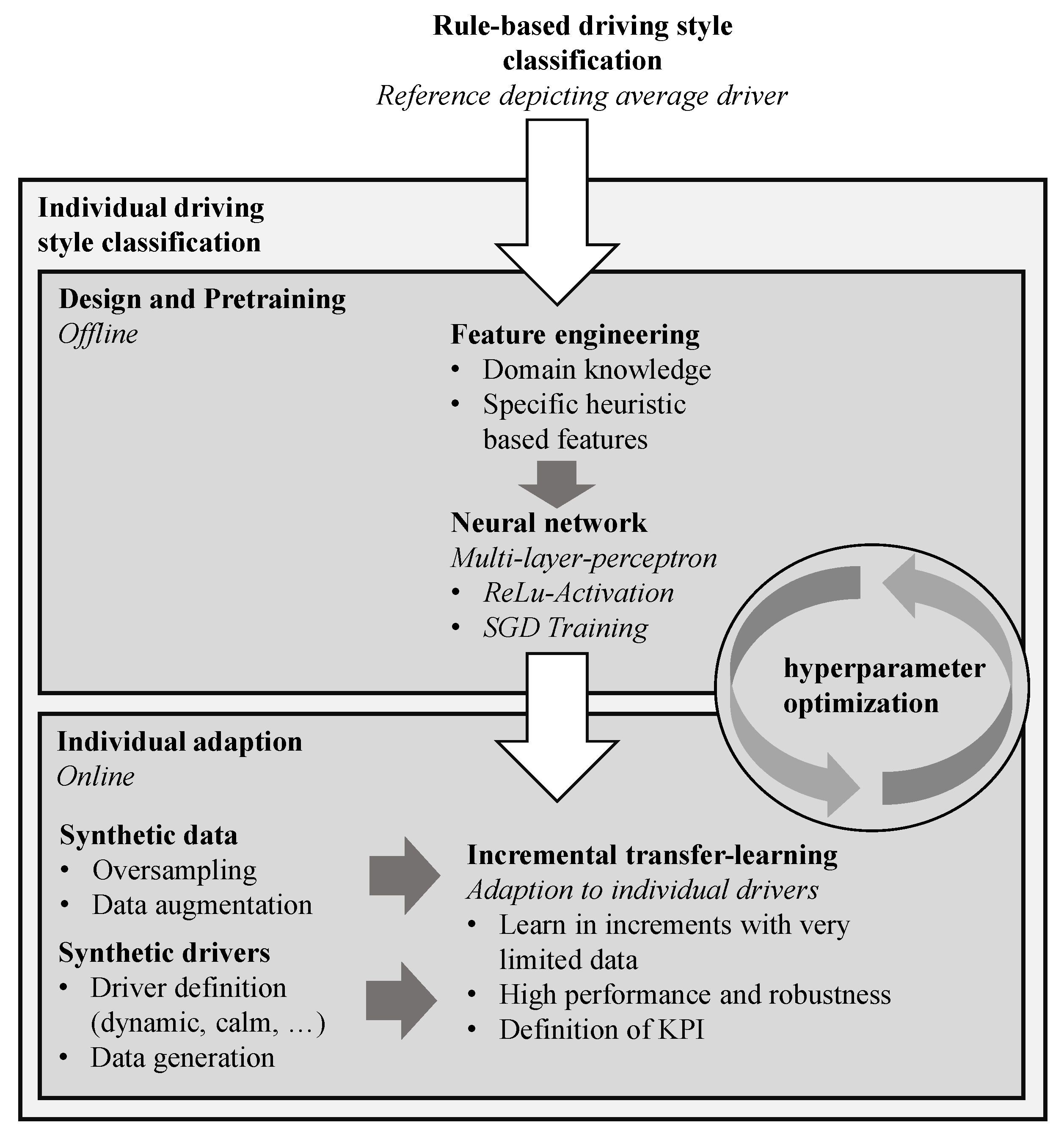
We propose a comprehensive individual driving style classification framework, which is composed as shown in Figure 1. The reference is a rule-based classification, which has been previously described by the authors.

First, the neural network design and pretraining for transfer learning have to be carried out. To improve the correlation between the input data and output labels, we engineered the neural network input features based on domain knowledge and experience. Therefore, instead of using raw time series data as an the input, we can provide specific heuristic-based features, which contain the necessary information for classification in a compressed way.

Then, we designed a neural network architecture that comes with a relatively low amount of parameters, whilst being able to achieve high performance on the classification task. That is important for robust transfer learning on limited data and was achieved through an hyperparameter optimization, which incorporated the entire individual classification framework. The selected network architecture was trained with stochastic gradient descent to act as an initial parametrization for online transfer learning.

The individual adaption through transfer learning was carried out in an online setting, where new labeled data were provided in increments. These labels were the result of a driver–vehicle interaction and may be acquired as secondary information from a vehicle function. Within our work and instead of human drivers, we define synthetic drivers, which represent dynamic, calm, or average driving style perceptions. By doing so, we were able to achieve consistent and reproducible results and were able to show the algorithm’s ability to improve for individual drivers. We also define drivers who give non-causal feedback and show that our algorithm does not diverge in the case of such input data. As a drawback, we were not able to account for exogenous influencing factors on the driving style perception of human drivers. For example, a human driver may perceive a dynamic driving style in the morning differently than in the afternoon. Such influencing factors shall be addressed for future practical application in wide-spread field studies.

By performing transfer learning on small amounts of data and by considering different synthetic drivers, concept drift is introduced. First, the probability distribution of the training data labels varies over time. Whilst we expect the driving style to be equally distributed in the case of the reference driver, for drivers who perceive the driving style in a more dynamic way, we expect a different distribution. Second, due to the low sample size of the training data, concept drift is introduced stochastically due to the randomness of the sample selection. If transfer learning is carried out solely on the small target domain sample, a high variance of the training metrics is expected due to these considerations. Therefore, we performed data augmentation with an oversampling algorithm, which uses synthetic driving data to improve the overall robustness for the described transfer learning setting.

3. Neural Network Design

In the following section, first, the feature engineering process is described. Then, we design a multi-layer perceptron with regard to the specific requirements of the transfer learning task. Finally, we perform a hyperparameter optimization using the Lichtenberg high-performance computer of the TU Darmstadt, which incorporates the entire individual driving style classification framework.

3.1. Feature Engineering

Neural networks with a sufficient size are theoretically able to map arbitrary functions [16]. However, when training these networks, problems such as vanishing gradients or convergence to local minima might inhibit good results depending on the underlying problem formulation and available data. For that reason, it is important to design a neural network with regard to the specific requirements of the learning task. Here, a key step is to create strong features with dense information and high correlation to the respective labels. This process is also known as feature engineering [17] and is covered in the following section.

For this, we used domain knowledge in the form of the results of our previous work, where we developed a heuristic rule-based driving style classification algorithm. There, we aggregated longitudinal and lateral acceleration data over time and used these two-dimensional profiles as the base for the classification rule. Through this process, the time series data were compressed whilst the results showed that the information about the driving style was still preserved [8].

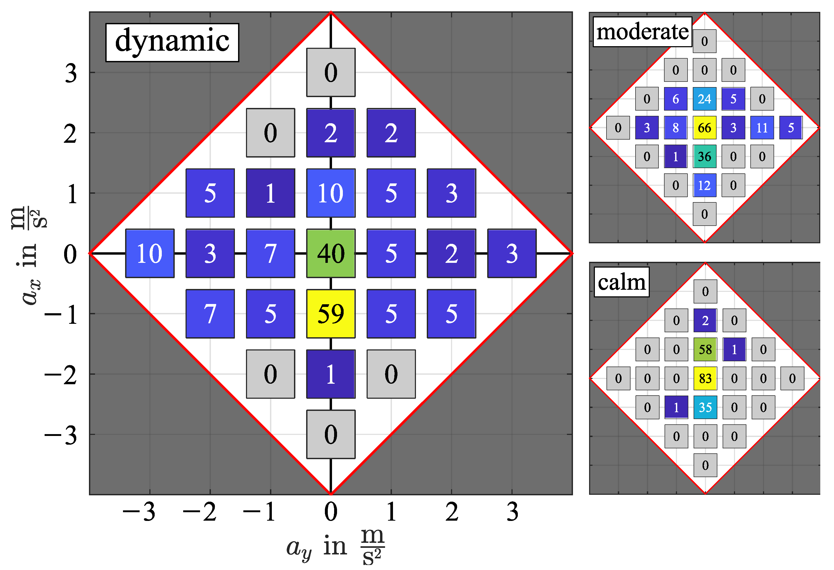
From these findings, we derived the specific and heuristic-based features for the proposed neural network. Figure 2 shows aggregated acceleration profiles for dynamic, moderate, and calm driving. For the aggregation, a fixed number of time series elements (here: 180, which correspond to $90\mathrm{s}$ at $\Delta t=0.5\mathrm{s}$) were sampled and sorted into the nearest acceleration bins. The bins have to be selected such that their number is reduced to a minimum whilst preserving important driving style information. That was accomplished by neglecting high combined acceleration values, which rarely occur (dark gray region). Values that lie within this region are sorted into the nearest bins inside the white region. The bin centers are defined as a result of the parameter optimization (here: $-3\mathrm{m}/{\mathrm{s}}^2-3\mathrm{m}/{\mathrm{s}}^2$ in lateral $a_x$ and longitudinal acceleration $a_y$ with $\Delta a=1\mathrm{m}/{\mathrm{s}}^2$ between bin centers). These parameters were chosen for vivid visualization and were different for the actual application.

The feature generation was carried out on a moving window basis as a First In, First Out (FIFO) buffer. At time $t_i$ and with a time window T, the data from $t_{i-T}$ until $t_i$ were used. At time $t_{i+1}$, the data from $t_{i-T}$ were removed from the buffer, whilst the data of $t_{i+1}$ were added. For the neural network inference and training, the displayed data were reshaped into a 1D array. By doing so, we were able to design a neural network without recurrence since the relevant temporal information was already present inside the features. Hence, we were able to apply simple and efficient neural network architectures.

As shown from our previous work, the vehicle speed is another important feature for driving style classification. That is because the vehicle acceleration is generally lower at higher speeds (e.g., highway driving) and, thus, the vehicle speed needs to be considered when evaluating the acceleration profile [15]. Thus, we provide the vehicle speed at evaluation time $t_i$ as an additional feature.

For future work, it may be investigated if it is useful to include further measures in the feature engineering process. These might be vehicle-specific measures such as jerk, accelerator pedal position, or non-vehicle-specific information such as weather data or the personal data of the driver. However, by including new inputs, the required amount of data for performing transfer learning will increase as well. Therefore, the use of such additional information has to be weighted against the required user data, which are sparse.

3.2. Training Data for Pretraining

Good training data are the key for successful supervised learning applications. However, in the case of driving style classification, these labeled data are generally not available. It is extremely expensive and time consuming to collect sufficient online labeled data for robust training. That is why we chose a different approach. Since our objective was to develop an adaptive driving style classification based on neural networks, we needed a good initial guess for the network weights to perform transfer learning. Therefore, we were able to make use of our previously described rule-based driving classification algorithm for initial training data generation.

For that, we equipped a Volkswagen Passat GTE with a data logger and collected about 10,000 km of unlabeled naturalistic driving data. The vehicle was used on a regular basis by different people, which resulted in a high variance of the driving situations. Over several years, these data was recorded in Germany by drivers of different experience levels. They include a variety of weather conditions in the different seasons, as well as day and night driving. It should be noted that the data are not representative of an average German driver, as they contain only official journeys and, for example, ≈50% of the kilometers were driven on freeways. However, this is of little importance for the present application, since the data were labeled automatically by a rule-based algorithm, which itself was based on representative data [8]. The data were classified into the three driving style classes with an approximately even label distribution: calm, moderate, and dynamic. The algorithm was used to train and test the neural network, as well as the developed features. Through that, the neural network was fit to replicate the mapping of our rule-based approach, which provides a good initial starting point for a later adaption.

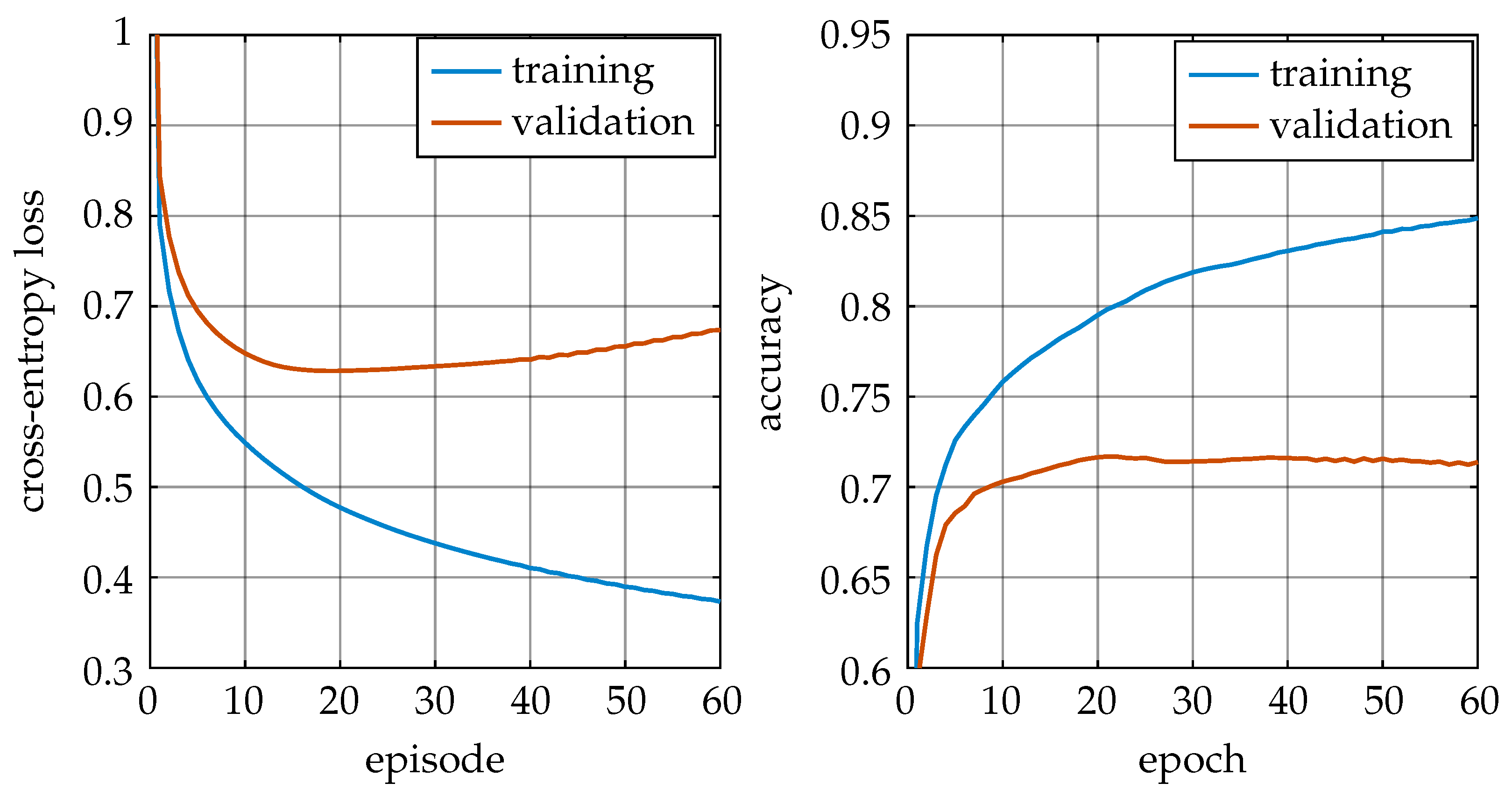
Figure 3 shows the pretraining metrics for initializing the network weights. As shown, a minimal validation loss was reached after approximately 20 episodes at a loss of ≈0.62 and an accuracy of ≈0.72.

3.3. Calibration through Temperature Scaling

The neural network output was calculated through the Softmax function, and the training data were one-hot-encoded. This resulted in an output vector with a sum of one and only positive elements. Hence, it might be tempting to interpret the neural network output directly as class probabilities. These probabilities are of high relevance for practical applications since they provide information on how confident the neural network is about certain inputs.

However, these output values generally do not correspond to the neural network confidence since it might suffer miscalibration [18]. Often, the neural network is miscalibrated such that it is too confident concerning its outputs, which may lead to false interpretation.

Figure 4 shows the confidence vs. accuracy for the pretrained network on the validation data. Here, the blue bars correspond to the network output before calibration. If the neural network is confident (80–100%) about a certain class, it can be observed that the actual accuracy within this confidence region is below that value. This means that the neural network overestimates its confidence.

A powerful and, yet, simple solution to this problem is Temperature scaling (T-scaling), where the input $z_i$ to the Softmax function ${\sigma }_{\mathrm{SM}}$ is scaled with an optimized temperature constant T [18]. The optimal temperature is calculated from minimizing the cross-entropy loss function on the validation set.

$$\begin{array}{c}\hfill \widehat{q_i}={\sigma }_{\mathrm{SM}}(z_i/T)\end{array}$$

(1)

To ensure an improved calibration, the estimated and maximum calibration errors [18] were calculated with and without T-scaling, as shown in

Table 1. Estimated and maximum calibration error (ece and mce).

	No T-Scaling	T-Scaling
ece	$2.68$	$1.41$
mce	$9.98$	$4.83$

. From that, a significant improvement in both errors can be observed. This improvement is further shown in Figure 4, where the change through T-scaling is shown by the hatched surface.

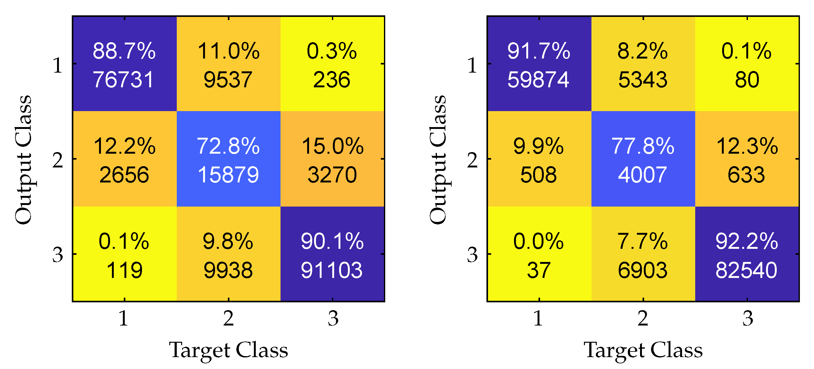
Figure 5 shows the classification confusion matrices with and without T-scaling. For that, the classification was carried out with an emphasis on high precision, which is the number of correctly classified elements per class divided by the total amount of elements in that output class. To achieve high precision, the output of the Softmax function is only accepted if the confidence is higher than $0.8$. Thus, not necessarily all inputs lead to a valid classification. As shown, through calibrating the model with T-scaling and by only accepting high confidence elements, the classification precision was improved in all three classes.

3.4. Neural Network Architecture

The selection of appropriate neural network architectures highly depends on the individual requirements. Within this work, transfer learning on limited data was carried out. For that reason, we focused on neural network architectures that have a low amount of free parameters to achieve robust training. Since the temporal dependencies of the driving style were already considered through the feature engineering process, the features at a single time step give adequate temporal information for the classification. A simple Multi-Layer Perceptron (MLP) with Rectified Linear units (ReLu) as activations is sufficient for this application [16].

Before conducting hyperparameter optimization, the key parameters and properties of the neural network architecture were fixed and were not further evaluated. That was performed based on experience and preliminary work. Due to our engineered features, we expected the neurons in the first layer to converge to generalized features (see Section 3.1). To enhance the incremental transfer learning, we introduced a scaling factor for the learning rate, which was unique for each layer, ${\lambda }_{\mathrm{scaler}}$. By doing so, we ensured that the pretrained generalized knowledge was preserved through training. We decided to add an additional hidden layer to process these features, such that our network was composed of one input, two hidden, and one output layers. Due to performing the classification task with one-hot encoding, we set the output layer to be Softmax and the loss function to be cross-entropy [19] (see

Table 2. Preset neural network architecture.

Concept	MLP (two hidden layers)
Input	Standardized 1D array
Activation Function	ReLu
Output	Softmax
Loss	Cross-entropy

).

3.5. Hyperparameter Optimization

We performed the hyperparameter optimization based on a two-step random grid search, where we first examined the entire parameter space and then concentrated on the found optimum. The optimization included the pretraining and the later-described incremental transfer learning. By doing so, we ensured that the identified parameters were not only optimal regarding the pretraining, but also regarding the incremental learning.

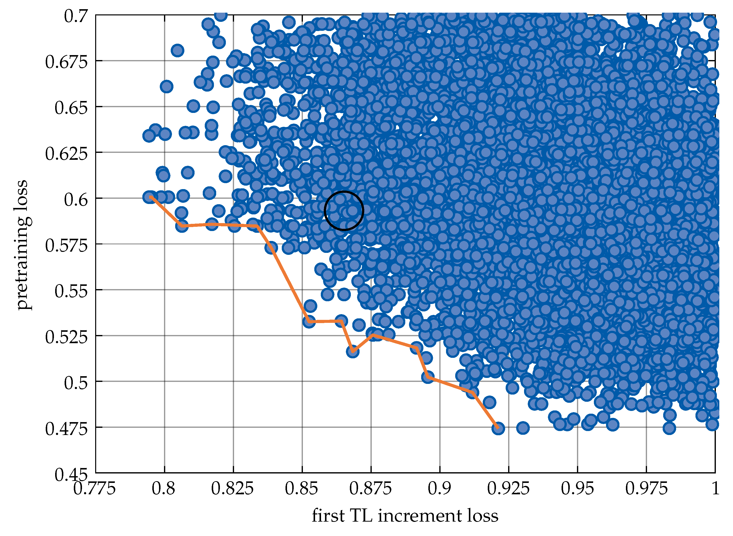
This approach is supported by Figure 6, which shows the Pareto front between reaching low pretraining losses and, at the same time, low transfer learning losses in the first increment. If we only optimized with regard to low pretraining losses, we would select a suboptimal solution for the incremental transfer learning, and vice versa.

However, for selecting the optimal parameter set, we needed to introduce an additional objective, which measures the robustness of the transfer learning. We performed this by executing the transfer learning process $N=250$ times. Due to the random sample selection process, every execution will give different results. To measure the robustness, we compared the loss on the reference and individual dataset in each increment and took the maximum value of the 95% quantile. By doing so, we ensured that the training method reached acceptable performance either on the reference data or on the individual target data in the majority of executions.

Through evenly weighting the described objectives (pretraining loss, transfer learning loss, robustness measure), we selected the optimal hyperparameter set as shown in

Table 3. Optimal hyperparameter random grid search.

	Range	Selected
aggregation horizon in s	$\{300,350,400,450,500,550\}$	500
aggregation resolution ${\mathit{a}}_{\mathbf{x},\mathbf{y}}$ in m s${}^{-\mathbf{2}}$	$\left\{\right[-6:1:6],[-5:1:5],$ $[-6:2:6],[-4:2:4]\}$	$[-6:2:6]$
aggregation resolution $\mathit{v}$ in m s${}^{-\mathbf{1}}$	$\left\{\right[0:20:40],[0:40:40],$$\left[0\right]\}$	$\left[0\right]$
number of neurons	${\{2,4,8,16,32\}}^2$	$[32,4]$
learning rate $\mathbf{\lambda }$	$\{0.01,0.0375,0.075,0.15\}$	$0.0375$
learning rate scaling ${\mathbf{\lambda }}_{\mathbf{scaler}}$	$\left\{\right[0.05,0.125,1],[0.1,0.25,1],$ $[0.25,0.5,1],[1,1,1]\}$	$[0.05,0.125,1]$
oversampling conv. constant ${\mathit{c}}_{\mathbf{ovs}}$	$\{0,0.05,0.15,0.3,0.5,0.75,1\}$	$0.3$

and marked in Figure 6.

4. Training Data for Transfer Learning

In the following sections, we discuss the generation of the data for our transfer learning framework. First, we created a synthetic driver model, which was used to gain the data for individualization. Then, we discuss the generation and selection of synthetic data for oversampling.

4.1. Synthetic Driver Model

As described in Section 2, we used synthetic drivers for generating training data for the validation of our approach. The aim was to generate drivers who perceive driving style differently. That was achieved by using the rule-based classification [8] on a reference dataset with different parameters depending on predefined requirements.

For our studies, we define the following driver types who perceive the reference driving situations:

• Driver 1: more dynamic (calm driver, share: $[10\%;20\%;70\%]$);
• Driver 2: average (average driver, share: $[33\%;33\%;33\%]$);
• Driver 3: more calm (dynamic driver, share: $[70\%;20\%;10\%]$);
• Driver 4: not reproducible (non-causal driver, share: $[33\%;33\%;33\%]$);

It shall be clarified that a driver who perceives the reference driving situation, for example, as more dynamic is generally described as a calm driver. That is because he/she has a lower tolerance for high driving dynamics measures and, thus, rates the reference more often to be dynamic.

For data generation, we used the rule-based classification and executed it on the reference data. This resulted in an evenly distributed driving style classification in the format of a time series. In the second stage, we processed that result in a PT1 filter and classified the individual driving style based on driver-specific parameter sets (see Equations (2)–(4)).

$$\begin{array}{cc}\hfill s{t}_{\mathrm{rb}}& \in \{1\equiv \mathrm{calm};2\equiv \mathrm{average};3\equiv \mathrm{dynamic}\}\hfill \end{array}$$

(2)

$$\begin{array}{cc}\hfill s{t}_{\mathrm{pt}1}^{k+1}& =s{t}_{\mathrm{pt}1}^k+c_{\mathrm{pt}1}\Delta t(s{t}_{\mathrm{rb}}^k-s{t}_{\mathrm{pt}1}^k)\hfill \end{array}$$

(3)

$$\begin{array}{cc}\hfill s{t}_{\mathrm{ind}}& =\left\{\begin{array}{cc}1\hfill & \mathrm{for}s{t}_{\mathrm{pt}1}<c_{\mathrm{low}}\hfill \\ 2\hfill & \mathrm{for}s{t}_{\mathrm{pt}1}>c_{\mathrm{low}}\wedge s{t}_{\mathrm{pt}1}<c_{\mathrm{up}}\hfill \\ 3\hfill & \mathrm{for}s{t}_{\mathrm{pt}1}>c_{\mathrm{up}}\hfill \end{array}\right.\hfill \end{array}$$

(4)

with $c_{\mathrm{low}}$ and $c_{\mathrm{up}}$ denoting the specific parameters for the generated drivers, which were selected such that the desired driving style distribution was reached.

4.2. Synthetic Data for Oversampling

A key requirement of our transfer learning framework was to be able to learn with very little individual data. As shown in the literature, a possible way to ensure robust learning in such settings is to use data augmentation to enlarge the dataset. We performed this by generating synthetic data to perform the oversampling with regard to the target domain dataset.

These synthetic data were generated through a Markov chain algorithm, which was described in [7]. We used approximately 10,000 km of real-world driving data and aggregated these data in longitudinal and lateral acceleration, as well as the speed direction. This was performed by first defining grid vectors and then sorting the time series elements into their respective bins. Additionally, we tracked the state transitions and calculated the transition probability matrix (tpm) to interconnect the aggregated profile. Now, we start off at a random point in the $a_x,a_y,v$-plane and move towards the next state by randomly sampling according to the tpm. By doing so, we can generate an arbitrary large dataset, which is always based on states and transitions occurring in real-world driving data.

With the help of the described process, we generated approximately ${10}^6$ km of synthetic driving data. Within the adaptive driving style classification framework, we used these data to perform oversampling. For that, we needed to find synthetic data segments that were similar to the actual segments that were present in the training set. Therefore, we needed a measure for time series similarity. Using the Euclidean distance for this task is straightforward, but comes with a major drawback. If the compared data are slightly shifted in the time domain and, other than that, have similar trajectories, the Euclidean distance will give high values, whilst the similarity score should be high for our application. We solved this problem by applying dynamic time warping (dtw), which is widely described in the literature [20].

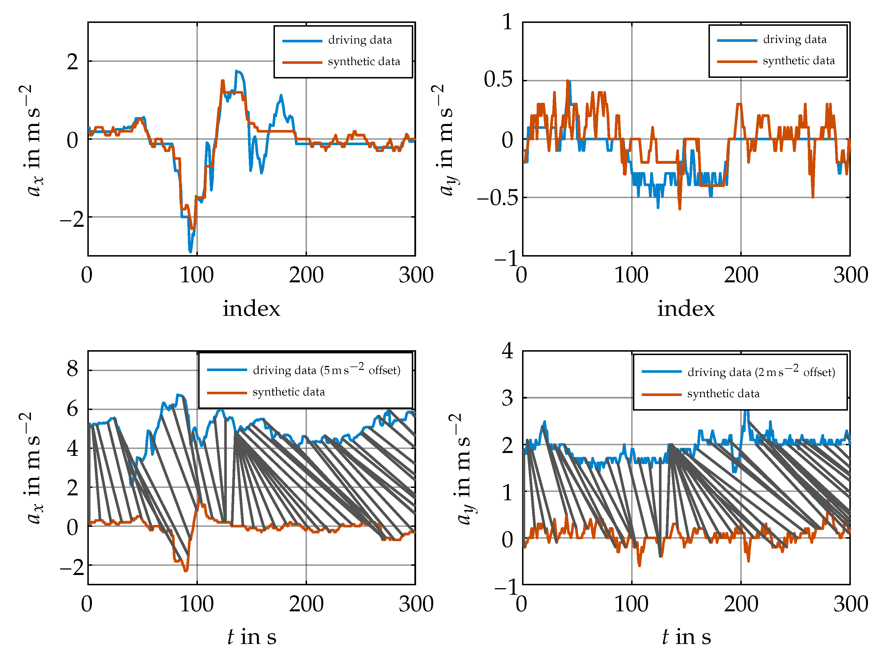
Figure 7 shows a two-dimensional time warping example for $a_x$ and $a_y$. For calculating the distance according to dtw, the raw data were warped in time by calculating a single time warping vector, which interconnected the data for comparison. The resulting warped sequences are shown on the top of the plot and the underlying data on the bottom. As shown, the Euclidean distance of the warped sequences was low, thus meaning that dtw would give a high similarity measure. The original driving data in the bottom graph are displayed with an offset for better readability. Here, the warping pattern is indicated by the gray lines. It is shown that, whilst the features of the compared original sequences were similar, the raw Euclidean distance would be high due to an offset in the time domain.

5. Incremental Transfer Learning

After introducing the boundary conditions of our adaptive driving style classification framework, we now focus on its design and on specific problems. A key feature of the proposed classification algorithm is its ability to learn with a low amount of data and in increments. That is, at each increment, we acquired three new training ($n_{\mathrm{tr}}=3$) and validation examples ($n_{\mathrm{val}}=3$). In future increments, we then trained with all data available to this point in time. Achieving improved classification results and high robustness on the test dataset with limited data were then the key objectives.

5.1. Oversampling

One problem that arises if training on such small datasets is that they are often highly unbalanced compared to the actual test data occurrence frequency distribution f. Training on these unbalanced datasets will prevent a robust classification improvement [21]. If, for example, performing transfer learning in the first increment on a number of $n_{\mathrm{tr}}=3$ examples and if expecting an evenly distributed test dataset, the probability for seeing a single label in all three examples is as high as $0.1$. In that case, however, no successful training would be possible, and the performance would decrease compared to the pretrained classification.

To overcome this problem, oversampling has been proposed by various literature works [6,22,23]. Through oversampling, the training and validation dataset distributions may be altered such that they meet the underlying test data distribution. However, in our application, this underlying test data distribution was generally unknown. We therefore used an evenly distributed standard reference for this work. With the help of oversampling, we generated a smooth transition from this reference to the actual training and validation distributions by using a PT1 filter.

First, we randomly selected $n_{\mathrm{tr}}\times N$ and $n_{\mathrm{val}}\times N$ samples, where N denotes the number of training increments. We then calculated the occurrence frequency distribution according to Equation (5) for each of the N increments $n_k^i$, where k indicates the dataset.

$$f_k^{\left(i\right)}=\sum _{j=1}^i\frac{n_k^j}{N}$$

(5)

Next, the target occurrence frequency distribution ${\mathit{f}}_{\mathrm{target}}^{\left(i\right)}$ was calculated by an iterative filter according to Equation (6). Here, ${\mathit{f}}_{\mathrm{target}}^{\left(i\right)}$ denotes the target distribution for the i-th increment and was initialized with a reference value. The actual distribution in training and validation samples is given by ${\mathit{f}}^{\left(i\right)}$. The filter convergence increased with the increments and is defined through the constant $c_{\mathrm{conv}}\in [0,1]$. Here, in the case of $c_{\mathrm{conv}}=0$, the target distribution remained at its initial value, whilst in the case of $c_{\mathrm{conv}}=1$, it was always set to the actual sample distribution.

$${\mathit{f}}_{\mathrm{target}}^{\left(i\right)}={\mathit{f}}_{\mathrm{target}}^{(i-1)}+min(c_{\mathrm{ovs}}i,1)({\mathit{f}}^{\left(i\right)}-{\mathit{f}}_{\mathrm{target}}^{(i-1)})$$

(6)

We then calculated the number of examples that had to be added to the training and validation datasets to meet the required target distribution. Based on these numbers, we added synthetic data that were similar to the available training and validation data by using dtw (see Section 4.2).

The oversampling convergence constant $c_{\mathrm{ovs}}$ was part of the hyperparameter optimization, and its conflicting influence on the robustness and transfer learning potential is shown in

Table 4. Oversampling convergence constant.

${\mathit{c}}_{\mathbf{ovs}}$	Robustness Measure		Transfer Learning Potential
	Normalized	Raw Value	Normalized	Raw Value
$\mathbf{0}$	1	$0.79$	0	$0.82$
$\mathbf{0.05}$	$0.96$	$0.81$	$0.64$	$0.76$
$\mathbf{0.15}$	$0.87$	$0.83$	$0.93$	$0.73$
$\mathbf{0.3}$	$0.75$	$0.87$	$0.98$	$0.73$
$\mathbf{0.5}$	$0.60$	$0.92$	$0.95$	$0.73$
$\mathbf{0.75}$	$0.05$	$1.08$	$0.98$	$0.73$
$\mathbf{1}$	0	$1.10$	1	$0.72$

. The values were the result of the hyperparameter optimization using a random grid search. Here, the robustness was measured as defined in Section 3.5. The transfer learning potential is the average mean of the first and last learning increment. If holding to the initial sample distribution ($c_{\mathrm{ovs}}\approxeq 0$), high robustness may be reached with the cost of low transfer learning potential. On the other hand, if no oversampling is performed ($c_{\mathrm{ovs}}\approxeq 1$), the robustness measure would decrease significantly, and at the same time, we would observe high transfer learning potential. The normalized quantities showed the benefit of the described oversampling since, with the result of the hyperparameter optimization, we achieved a high transfer learning potential ($0.98$) and, at the same time, high robustness ($0.75$).

5.2. Implementation of the Learning Algorithm

As of now, the training data acquisition, hyperparameter optimization, and oversampling for transfer learning have been described. Next, we develop the incremental transfer learning algorithm. Due to the low amount of data, there was no necessity for batch learning, and we carried out gradient descent.

Due to performing homogeneous transfer learning, we assumed that the first layer’s features learned by the neural network generalize well for the given task. From that knowledge and as a result of our hyperparameter optimization process, we decided to implement ascending learning rates for the neural network layers, which prevented a “catastrophic forgetting” [24] effect, especially in the first layers. This was achieved through a scaling factor ${\lambda }_{\mathrm{scaler}}$, which was applied to the computed gradients during training.

The training was then carried out on the oversampled training data and was stopped at a minimal validation loss. At each increment, all previous available data were taken into account, and training was thus started with the pretrained, initialized network weights. Since the learning task was stochastic due to the random selection of training and validation samples, it is simulated multiple times for reliable analysis in Section 6.

6. Results

To assess the proposed method, training was carried out with regard to the four individual drivers defined in Section 4. The results are shown in Figure 8, Figure 9, Figure 10 and Figure 11. Here, the initial pretraining metric is shown in red for Iteration 0. The training result of multiple runs as defined by Table 3 and

Table 5. Main parameters in the learning process.

# of training samples/increment	${\mathit{n}}_{\mathbf{tr}}=3$
# of validation samples/increment	${\mathit{n}}_{\mathbf{val}}=3$
# of simulation runs	$\mathit{N}=250$

is shown in box plots. Here, 50% of the data points for each increment lay within the boxes. The length of the whiskers is at a maximum $1.5$-times the height of the box, but less if no data points exist outside that range. The figures show the performance metrics on the individual driver’s data, as well as on the reference dataset. The accuracy was computed as described in Section 3.3 by calibrating the pretrained neural network and only accepting samples with a high confidence.

Figure 8 shows the results for Driver 1. As shown, his median loss improved monotonically from Increment 1 on. Thus, by solely training on three samples, we were already able to improve his metrics. We also observed that the performance metrics reached a saturation towards the end of training, which means that a further improvement after five transfer learning increments was not to be expected. Besides the performance on the individual data, a high robustness was desired. As previously defined, we evaluated the performance on both datasets and ensured that the high performance metrics were reached at least in one dataset. As shown, the reference metrics did not drop significantly from Increment 1 on; thus, the desired smooth transition from the performance on reference data towards individual data was achieved.

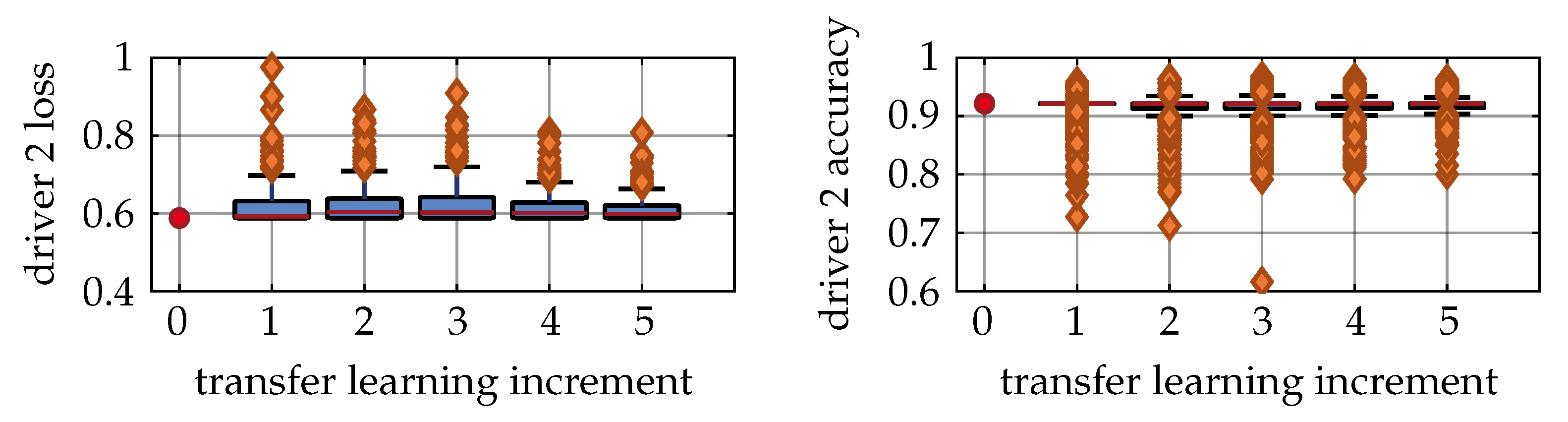
Figure 9 shows the training results for the reference Driver 2. His data were also used for pretraining; thus, we achieved high initial performance metrics. As expected, the majority of data points for all increments lied within a small interval of the initial metrics, and no further improvement was reached. Due to the random sample selection process, some training runs led to decreased performance metrics, which are shown as outliers. The number of outliers decreased with the number of increments, since the significance of the random sample selection process decreased as well.

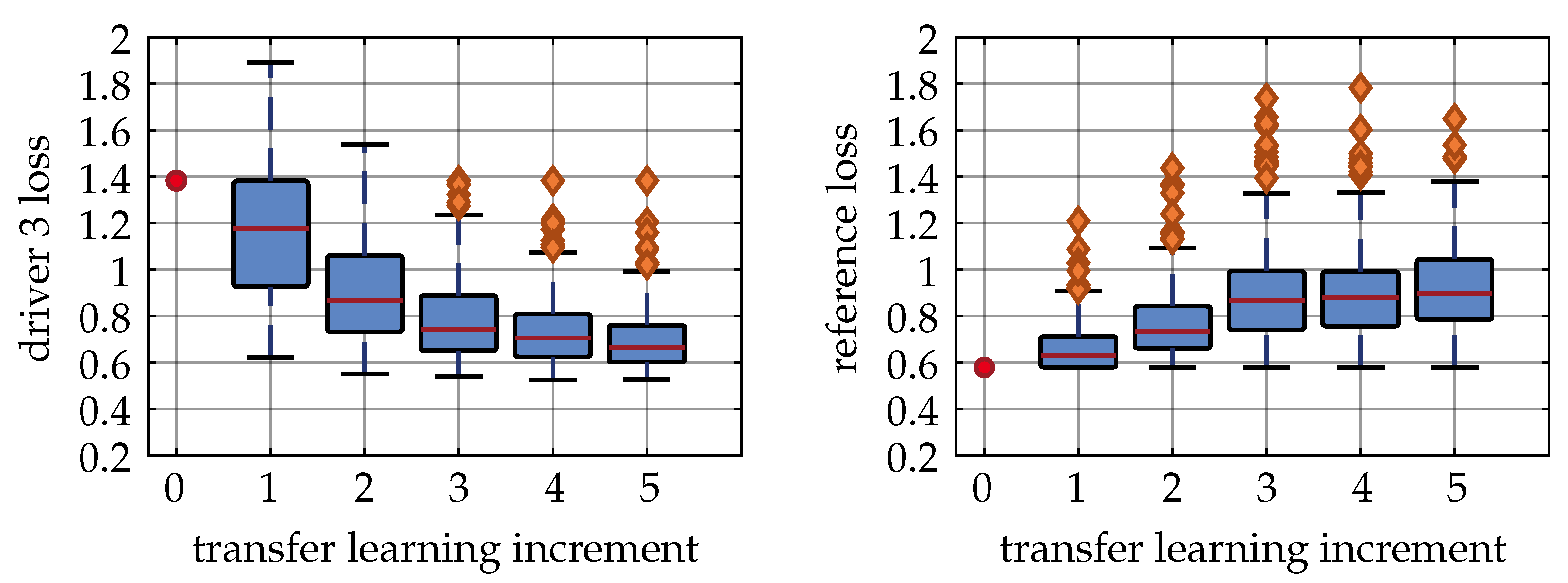
Figure 10 shows the training results for Driver 3. Here, a similar observation compared to Driver 1 can be made. Whilst the initial loss was at ≈1.4, it steadily decreased until it reached a mean loss of ≈0.6. At the same time, the reference loss increased from ≈0.6 to ≈0.9. We also observed the desired smooth transition from the performance on the reference data towards the performance on the individual dataset. Additionally, we can observe that the increase of individual performance was significantly higher in comparison to the decrease on the reference data.

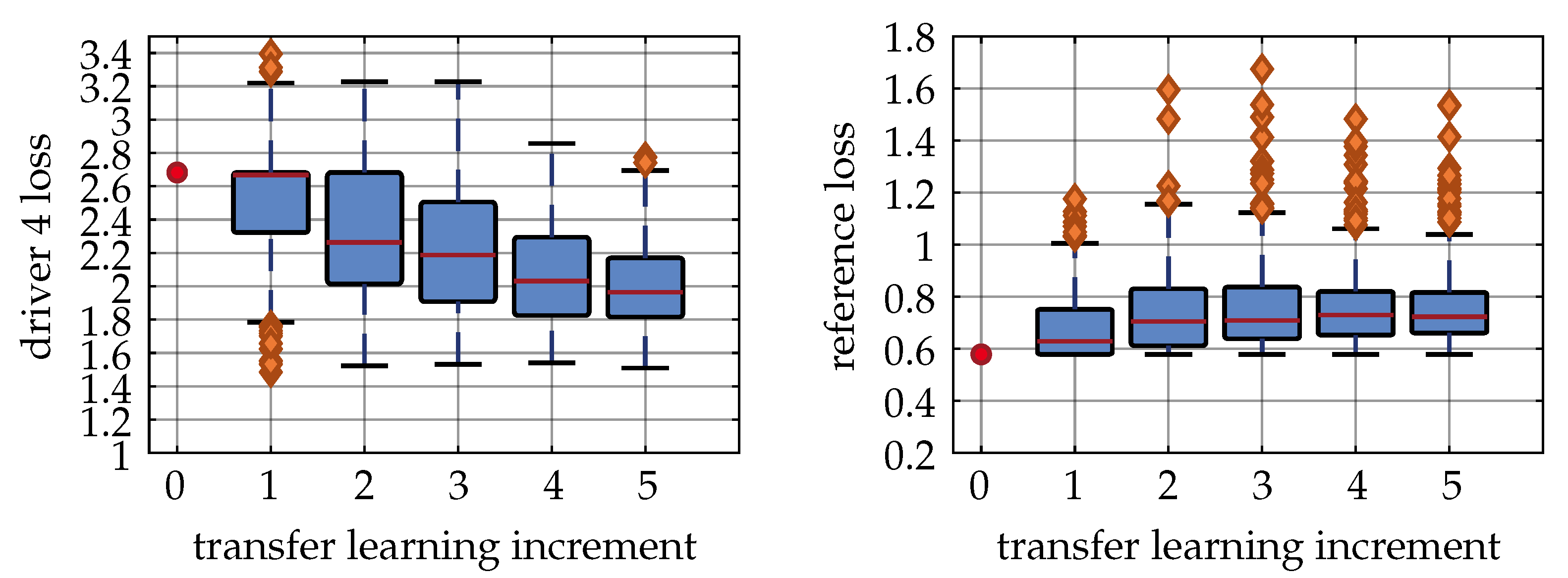
Figure 11 and

Table 6. Mean reference accuracy and share of valid classifications for the non-causal Driver 4.

Iteration	Mean Reference Accuracy	Valid Classifications
$\mathbf{0}$	$0.93$	$33\%$
$\mathbf{1}$	$0.87$	$32\%$
$\mathbf{2}$	$0.86$	$29\%$
$\mathbf{3}$	$0.86$	$27\%$
$\mathbf{4}$	$0.86$	$24\%$
$\mathbf{5}$	$0.87$	$22\%$

show the results for the non-causal Driver 4. They have to be analyzed differently compared to the previous drivers since, theoretically, no useful classification can be given with an expected accuracy of 33%. We used this driver to showcase the robustness of the described algorithm in the case of random inputs, which might occur in practical field application. First, Figure 11 shows that the individual loss was generally at a high level, but still decreased with the increments. That is because the best cross-entropy loss for random labels is defined by $log\left(3\right)=1.1$ and the neural network will converge towards this value. Other than that, the reference loss increased only slightly if compared to Drivers 1 and 3. Table 6 shows the reference accuracy and the share of valid classifications on the test set. That is the number of samples with a confidence higher than the previously defined value of $0.8$. We observed that, whilst the accuracy on the reference dataset remained high, the number of valid classifications decreased. This was the desired behavior since the best output for Driver 4 would be no output at all.

7. Discussion

The main challenge in the described adaptive driving style classification framework was the limited training data when training for individual drivers. With our results, we showed that, from the first increment on, we were able to increase the average accuracy for all reproducible drivers whilst achieving high robustness at the same time. Within this contribution, we showed that, through integrating various state-of-the-art machine learning methods, high system level performance and robustness were achieved even with so few training data.

The hyperparameter optimization results showed that, by using synthetic data oversampling and by transitioning from a reference label distribution towards the individual drivers distribution, the overall robustness increased significantly, whilst a good average loss was still preserved. Additionally, we showed that, by performing temperature scaling to calibrate the neural network to classify only samples with a high confidence, the overall accuracy increased. That is especially important for non-causal drivers, since the neural networks confidence decreased significantly if transfer learning on random data. Thus, for such drivers, the neural network will give less-valid classifications, which is desired, as we were theoretically not able to classify driving style in this case.

We also optimized the hyperparameters with regard to the entire framework. By doing so, we ensured that the found parameters were not solely optimal regarding the performance on pretrained data, but also for the actual application on system level. Here, we observed a conflict between high pretraining loss, high transfer learning potential, and high robustness and found the optimum by weighting these objectives evenly.

The shown results from our learning framework relied on the definition of synthetic drivers. Whilst this approach gives reproducible results for systematic validation, it lacks the complexity of real-life driving data. Here, further exogenous factors will influence the driver’s driving style perception and, through that, the transfer learning. Thus, for future work, the described adaptive driving style classification framework should be deployed for various test vehicles to perform a wide-spread study with different drivers in real-life driving scenarios.