Modeling of the Resonant Inverter for Wireless Power Transfer Systems Using the Novel MVLT Method

Abstract

Wireless power transfer (WPT) is a power transfer technique widely used in many industrial applications, medical applications, and electric vehicles (EVs). This paper deals with the dynamic modeling of the resonant inverter employed in the WPT systems for EVs. To this end, the Generalized State-Space Averaging and the Laplace Phasor Transform techniques have been the flagship methods employed so far. In this paper, the modeling of the resonant inverter is accomplished by using the novel Modulated Variable Laplace Transform (MVLT) method. Firstly, the MVLT technique is discussed in detail, and then it is applied to model a study-case resonant inverter. Finally, a study-case resonant inverter is developed and utilized to validate the theoretical results with MATLAB/Simulink.

1. Introduction

The Wireless Power Transfer (WPT) system transmits electrical energy without any physical connection [1]. WPTs offer various benefits over wired ones, making them ideal for industrial applications: reducing danger from exposed wires, rendering the charging process easy, and reliable power transfer in rough weather conditions [2]. WPT is accomplished by inductively coupling the transmitter and receiver coils [3], thanks to Faraday’s law of electromagnetic induction. The receiver coil is deployed in the vehicle chases while the transmitter coils are buried under the ground. Further, due to better efficiency, resonant inductive WPT is used for EV charging [4].

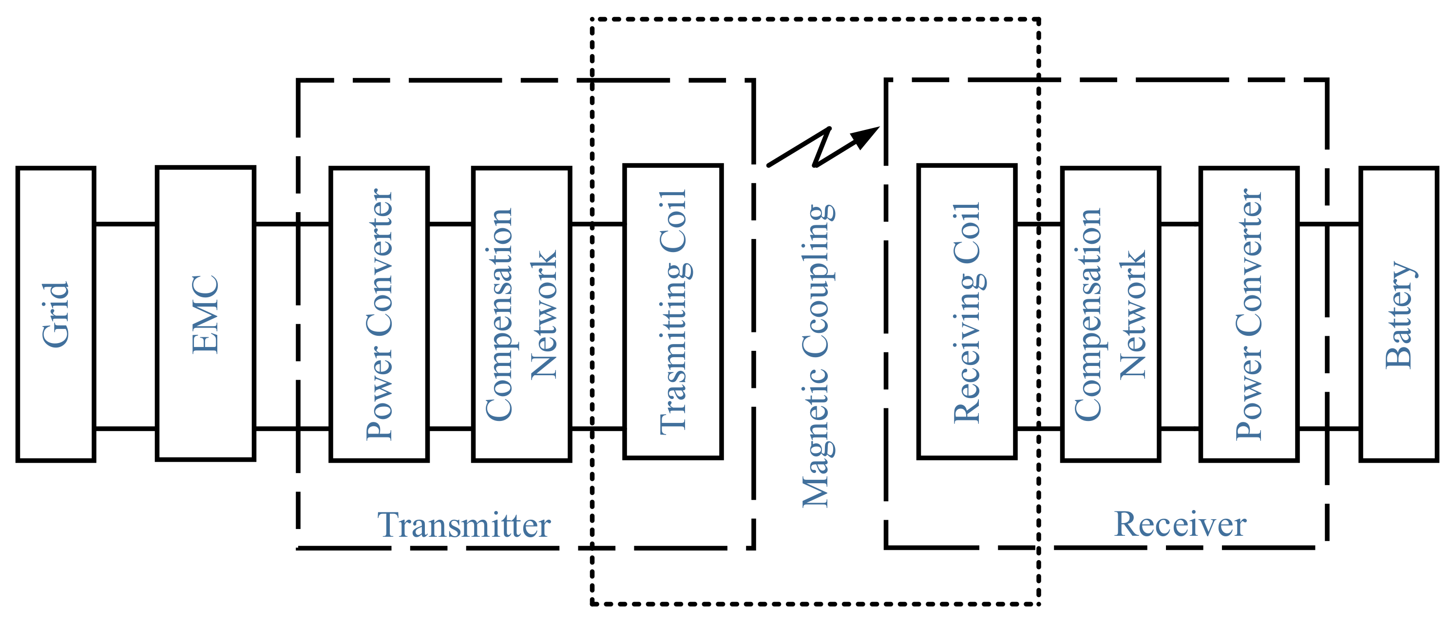
The schematic of a WPT system is shown in Figure 1. It is composed of various power conversion stages [1]. On the transmitter side, it consists of a power factor correction circuit (PFC) and a high-frequency inverter, whereas on the receiver side, it has an uncontrolled bridge rectifier and a chopper cascaded with it. Moreover, on the transmitting side, the electromagnetic compatibility (EMC) filter ensures that the system meets the electromagnetic standards. The filtered low-frequency grid voltage is applied at the input of the PFC circuit for rectification. Typically, PFC stands for power factor correction, and it is carried out by either a simple uncontrolled diode rectifier [5] or a controlled rectifier [6]. The inverter converts DC voltage into AC voltage, feeding power to the transmitter coil. The induced high-frequency voltage on the receiver coil is conditioned by the diode rectifier and the chopper to regulate the voltage and current profile suitable for battery charging [7]. In addition, the compensation network on both sides improves the system efficiency and cancels the reactive power demand from the inverter.

Usually, the steady-state analysis of a WPT system is carried out through the Fundamental Harmonic Approximation (FHA) technique [8]. For the transient analysis, instead, it is necessary to have a good dynamic model of the system available. To find the dynamic model of a WPT system, the traditional State-Space Averaging (SSA) method cannot be used because one prerequisite for its application is that the state variables of the system should be slowly time-variant compared to the converter switching period [9]. Furthermore, the transmitting power stage of a WPTS can be envisaged as a resonant converter. In resonant converters, the quantities in the resonant tanks exhibit predominantly oscillatory behavior. In WPTSs, the quantities involved in compensating networks are alternated signals pulsating at the inverter switching frequency. In other words, the switching period is equal to the natural time constant of the system. For this reason, SSA method applied to WPTSs and in general to resonant converters is not able to yield a useful dynamic model.

Therefore, other methods should be used to model the resonant inverter employed in the WPT systems, where its switching frequency is deliberately chosen to be close to the system natural frequency. To that end, the two main techniques that have gained success in the literature are the Generalized State-Space Averaging (GSSA) [10,11,12,13,14] and the Laplace Phasor Transform (LPT) [15,16,17,18,19]. These methods overcome the problem of the SSA technique by considering for the modeling of the AC quantities their slow-varying envelopes in place of their average values is refer [20,21]. A novel method called Modulated Variable Laplace Transform (MVLT) has been recently introduced by the author [22]. The method exploits the same averaging principle as the GSSA and the LPT techniques, and as demonstrated in [23], in the case of the modeling of a linear system, they are perfectly equivalent.

All the methods mentioned possess advantages and drawbacks. The GSSA method is the most general of the methods, but at the same time, it is relatively sophisticated due to the state-space representation of the system, which in some cases does not add any benefit to the analysis. The LPT is a circuit-based modeling technique that is relatively easy to apply, despite the usage of unconventional components such as complex resistors. In other words, the GSSA method applies the transformation to the state-space equations of the system, whereas the LPT method is based on transformations at the circuit level. The application of the LPT method starts with the conversion of the original circuit, substituting all the elementary components with their respective Laplace phasor-transformed counterparts. From the transformed circuit, it is easy to evaluate all the desired transfer functions.

This paper aims to show that in some situations, such as the modeling of the resonant inverter on the transmission side of the WPT systems, the MVLT technique could be the method to be preferred due to its simplicity and its straightforward application. The reason for the introduction of a new modeling method is that with both the GSSA and the LPT methods, the direct link between the instantaneous model and the envelope model is lost. This link is maintained by the MVLT method which thus can provide better insight into the envelope model.

This paper is organized as follows: Section 2 describes the WPT system to be modeled and the assumptions made to achieve this goal. Section 3 explains the MVLT method, and in Section 4, this method is applied to model the study-case resonant inverter. In Section 5, the model is verified by simulation. Finally, Section 6 concludes the paper.

2. System Description

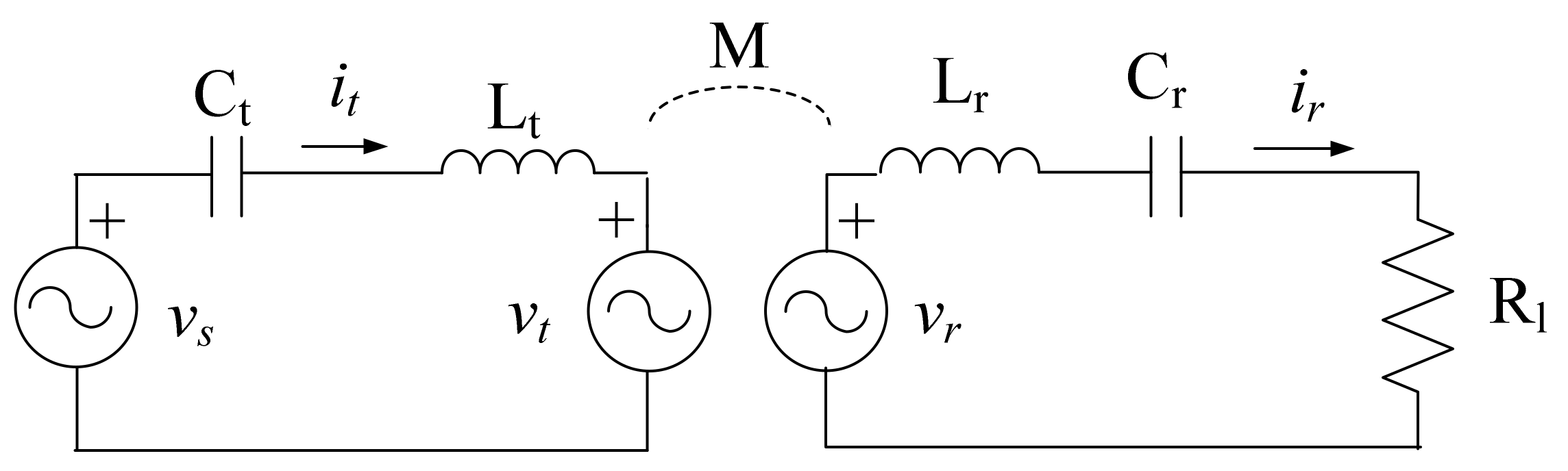
The equivalent circuital diagram of the WPT system with a series–series compensation network is illustrated in Figure 2. Here, vs. is the source voltage; v_t and v_r are the voltages induced on the transmitter and receiver coils, respectively. The induced voltage in the coil is caused by a change in current in the coil, which may be explained by Faraday’s law of electromagnetic induction. C_t, C_r, and L_t, L_r are the transmitter and receiver side capacitors and inductances, respectively; the transmitter and receiver components are identical. Further, i_t and i_r are the transmitter and receiver side currents, respectively, and M is the mutual inductance between the two coils. R_l is the resistance seen from the receiver coil. It is also referred to as load resistance.

From the analysis carried out in [23], the entire receiver side can be replaced by a resistance R reflected to the transmitter side and is given by

$$R=\frac{{\left(\omega M\right)}^2}{R_l}$$

(1)

Here, $\omega$ is the supply angular frequency in rad/sec, and is equal to $2\pi f$, where f is the supply frequency in Hz. It should be noted that the voltage vs. is controlled by the phase-shift method, in which the frequency f remains fixed at 85 kHz. The supply frequency was chosen in accordance with the SAE J2954 standard, which recommended the operating frequency range of 79–90 kHz for the WPT system for EVs.

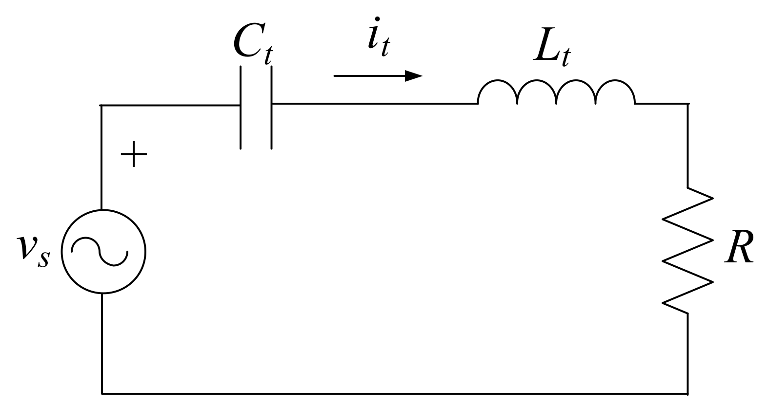
As may be observed from (1), that the receiver side reflects resistance to the transmitter side R depends on the values of M and R_l which vary with respect to the coil alignment and the battery state of charge, respectively. In this paper, for simplicity, M and R_l are considered to be fixed, thus giving a fixed value for R. In order to find an easy way to model the WPT system, the circuit of Figure 2 is redrawn in Figure 3, which can be represented as a simple series RLC network together with the load resistance R and source voltage v_s, in which the following hypotheses are made: (i) the inverter switching frequency f is the resonant frequency of the L_tC_t tank which follows the relation $f=\frac{1}{2\pi \sqrt{L_t{C}_t}}$; (ii) due to the filtering action of the L_tC_t resonating tank, the current i_t is nearly sinusoidal; (iii) although the supply voltage is a quasi-square, only fundamental component contributes in the power transfer. Since the harmonic content of the resonant converter output is low, we used fundamental wave analysis in this paper.

3. MVLT Modeling Method

The novel MVLT modeling method was first presented in [22], where the authors used this technique for the dynamic modeling of wireless power transfer systems. The technique can be applied to any circuit where the involved quantities are high-frequency sinusoidal signals with slowly varying amplitudes, like the ones illustrated in Figure 3. By applying a mathematical transformation, the MVLT method eliminates the high frequency and obtains a relationship between the envelopes. Supervising the envelopes of the quantities is easier due to their limited bandwidth, and at the same time, it is enough to maintain the system under control.

An amplitude modulated signal, e.g., $x\left(t\right),$ can be written in the form of its dynamic phasor $\overline{x}\left(t\right)$ [22] as

$$x\left(t\right)=\Re \left\{\overline{x}\left(t\right)e^{j\omega t}\right\}$$

(2)

Here $\Re \left\{·\right\}$ is the real part operator and $\omega$ is the angular frequency of the carrier of the modulated signal $x\left(t\right)$. As an assumption of the MVLT technique, the frequency content of $\overline{x}\left(t\right)$ should be negligible at frequencies approaching $\omega$, so that the modulating signal is much slower than the carrier. With this hypothesis, if $x\left(t\right)$ is provided as the input signal to a system having a transfer function $G\left(s\right)$, the output signal $y\left(t\right)$ can also be written in the form of (2). Hence, the relationship between the Laplace transforms of these two complex signals will be

$$\mathcal{L}\left\{\overline{y}\left(t\right)e^{j\omega t}\right\}\left(s\right)=G\left(s\right)\mathcal{L}\left\{\overline{x}\left(t\right)e^{j\omega t}\right\}\left(s\right)$$

(3)

where the operator $\mathcal{L}\left\{·\right\}$ is the Laplace transform of the argument. Using the “frequency shifting” property of the Laplace transform and with some additional mathematical steps, Equation (3) becomes

$$\overline{Y}\left(s\right)=G\left(s+j\omega \right)\overline{X}\left(s\right)$$

(4)

Here, the quantities $\overline{X}\left(s\right)$ and $\overline{Y}\left(s\right)$ are the Laplace transforms of $\overline{x}\left(t\right)$ and $\overline{y}\left(t\right)$, respectively. It is clear from (4) that the transfer function which links phasor quantities is nothing but the transfer function $G\left(s\right)$ of the original signals with $s$ mapped into $s+j\omega$. The transfer function $G\left(s+j\omega \right)$ is a rational function of $s$ with complex coefficients. Nevertheless, it is always possible to break (4) into its real and the imaginary parts, as explained in the Appendix A, and it results in

$$G\left(s+j\omega \right)=G_{Re}\left(s\right)+j{G}_{Im}\left(s\right)$$

(5)

where $G_{Re}\left(s\right)$ and $G_{Im}\left(s\right)$ are rational functions in $s$ with real coefficients in their numerators and denominators. Equation (4) gives the transfer function between the complex signals $\overline{x}\left(t\right)$ and $\overline{y}\left(t\right)$. However, the target is to find the relationship between the envelopes. In this regard, the envelope of the output signal $y\left(t\right)$, which is $\left|\overline{y}\left(t\right)\right|$, is given by

$$y_{env}\left(t\right)=\left|\overline{y}\left(t\right)\right|=\sqrt{y_{Re}^2\left(t\right)+y_{Im}^2\left(t\right)}$$

(6)

Here $y_{Re}\left(t\right)$ and $y_{Im}\left(t\right)$ are the real and imaginary parts of $\overline{y}\left(t\right)$. Since (6) is not linear, it needs to be linearized to get the transfer function between the envelopes of the output $y_{env}\left(t\right)$ and of the input $x_{env}\left(t\right)$. The linearization of (6) leads to

$$\left\{\begin{array}{c}{\overline{y}}_{env}\left(t\right)\approx \frac{Y_{Re,i}}{\sqrt{Y_{Re,i}^2+Y_{Im,i}^2}}{\tilde{y}}_{Re}\left(t\right)+\frac{Y_{Im,i}}{\sqrt{Y_{Re,i}^2+Y_{Im,i}^2}}{\tilde{y}}_{Im}\left(t\right) \\ \approx cos({\varphi }_i){\tilde{y}}_{Re}\left(t\right)+sin\left({\varphi }_i\right){\tilde{y}}_{Im}\left(t\right)\end{array}\right.$$

(7)

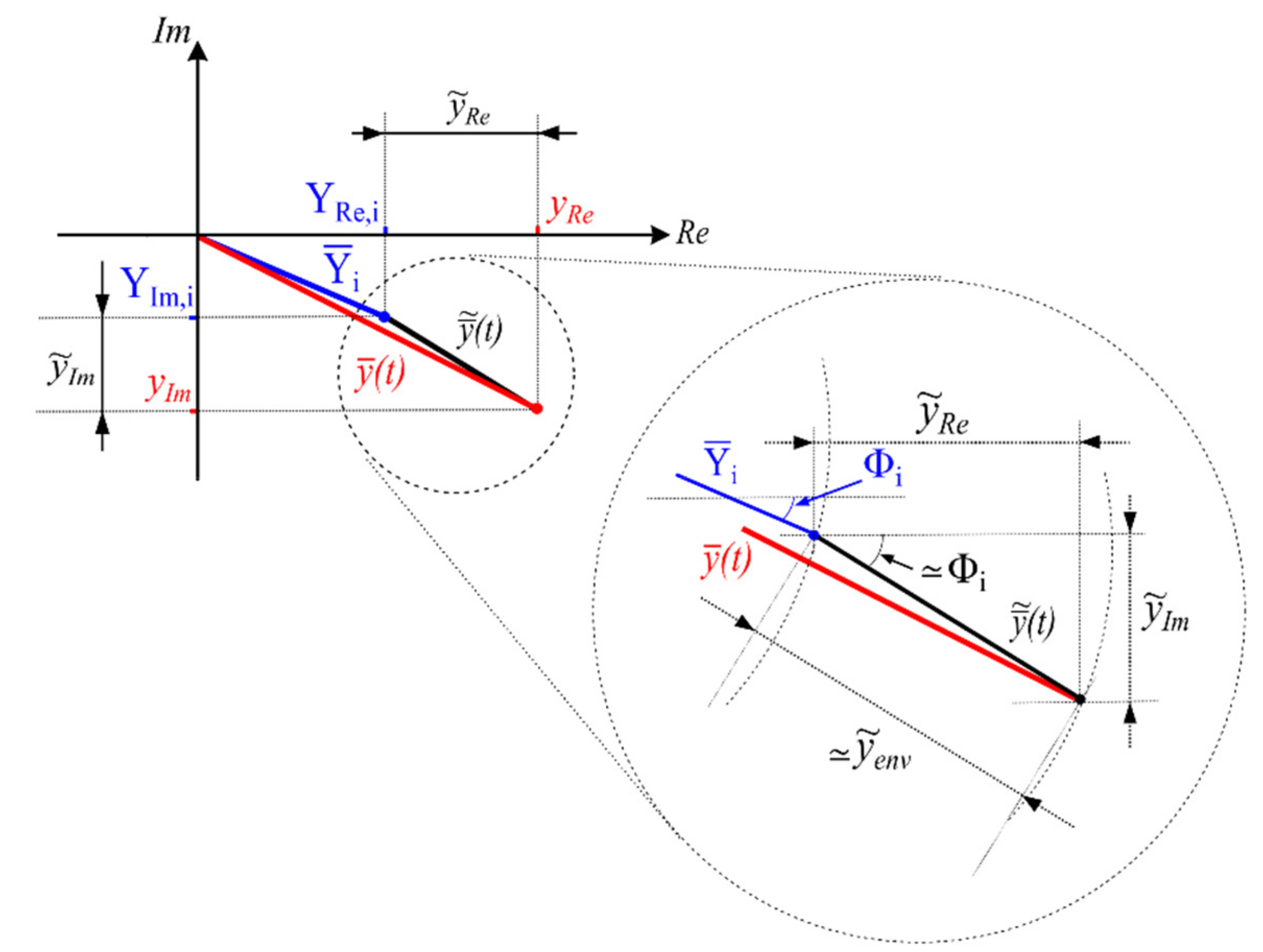
The graphical plot of Equation (6) for the linearization process of the output signal $y\left(t\right)$ is shown in Figure 4. Indeed, the envelope of the output signal $y\left(t\right)$ in linearized form is represented in Equation (7). Where subscripts i and f stand for the “initial” and “final” operating points, $Y_{Re}$ and $Y_{Im}$ are the real and imaginary parts of ${\overline{Y}}_i=Y_i{e}^{j{\varphi }_i}$, where ${\overline{Y}}_i$ represent initial output of signal $y\left(t\right)$ with blue phasor with ${\varphi }_i$ angle, which coincides with the conventional phasor of the output $y\left(t\right)$ before the perturbation that can be represented with a red phasor. The process of linearization can be better appreciated in Figure 4. The dynamic phasor $\overline{y}\left(t\right)$ moves from its initial value ${\overline{Y}}_i$ to the final value ${\overline{Y}}_f$. During the transient, $\overline{y}\left(t\right)$ can be written as ${\overline{Y}}_i+\tilde{\overline{y}}\left(t\right)$, where $\tilde{\overline{y}}\left(t\right)={\tilde{y}}_{Re}+j{\tilde{y}}_{Im}$ identifies its small variation around ${\overline{Y}}_i$ in the complex plane that can be represented with a black phasor. Assuming insignificant change in ${\varphi }_i$ so that the phase of $\overline{y}\left(t\right)$ remains almost constant for all the transition, from Figure 4, the second equality of (7) appears more clear. Applying the Laplace transform to (7) and neglecting the tildes for the sake of lightening the notation, Equation (8) is obtained.

$$Y_{env}\left(s\right)=cos({\varphi }_i)Y_{Re}\left(s\right)+sin\left({\varphi }_i\right)Y_{Im}\left(s\right)$$

(8)

To link the Laplace transform of $Y_{Re}\left(s\right)$ and $Y_{Im}\left(s\right)$ to the Laplace transform of the small-signal input, let us consider the carrier of the signal $\tilde{x}\left(t\right)$ as the reference of the phases. As a result, the dynamic phasor $\tilde{\overline{x}}\left(t\right)$ given by ${\tilde{x}}_{Re}\left(t\right)+j{\tilde{x}}_{Im}\left(t\right)$ consists of the real part only. Therefore, with this frame of reference, the real part of $\tilde{\overline{x}}\left(t\right)$ also coincides with its envelope, and consequently $X_{env}\left(s\right)$ is equal to $X_{Re}\left(s\right)$ in the $s$-domain. When $\tilde{\overline{x}}\left(t\right)={\tilde{x}}_{Re}\left(t\right)$ is applied to $G\left(s+j\omega \right),$ the dynamic phasor $\tilde{\overline{y}}\left(t\right)$ is obtained. Since the input of $G\left(s+j\omega \right)$ is real, the real part of $\tilde{\overline{y}}\left(t\right)$ is the output of $G_{Re}\left(s\right)$ and the imaginary part is the output of $G_{Im}\left(s\right)$. With this consideration, Equation (8) becomes

$$Y_{env}\left(s\right)=[cos({\varphi }_i)G_{Re}\left(s\right)+sin\left({\varphi }_i\right)G_{Im}\left(s\right)]X_{env}\left(s\right)$$

(9)

Considering that the function enclosed in the square brackets can be obtained as $\Re \left\{G\left(s+j\omega \right)e^{-j{\varphi }_i}\right\}$, provided that $s$ is assumed to be real [14], the transfer function linking the envelopes can be finally written as

$$G_{env}\left(s\right)=\frac{Y_{env}\left(s\right)}{X_{env}\left(s\right)}=\Re \left\{G\left(s+j\omega \right)e^{-j{\varphi }_i}\right\}$$

(10)

It is interesting to note that the angle ${\varphi }_{\mathrm{i}}$ of the phasor ${\overline{Y}}_i$ is also the phase of $G\left(j\omega \right)$. From (10), it is easy to see that the MVLT method, applied to a linear system, directly relates the transfer functions for the modulated quantities and the transfer functions for the modulating signals (the envelopes). In the Appendix A, this relationship is further analyzed.

4. Method Application

As a first step for the MVLT method application, the transfer function between the original signals of the equivalent WPT system of Figure 3 is evaluated. For instance, the transfer function between current i and the input voltage source vs. is

$$G_i\left(s\right)=\frac{I\left(s\right)}{V_s\left(s\right)}=\frac{s{C}_t}{1+sR{C}_t+s^2{L}_t{C}_t}$$

(11)

As a second step, mapping $s$ into $\left(s+j\omega \right)$ in (11) gives

$$G_i\left(s+j\omega \right)=\frac{s{C}_t+j\omega C_t}{L_t{C}_t{s}^2+\left(R{C}_t+j2\omega L_t{C}_t\right) s+\left(1-{\omega }^2{L}_t{C}_t+j\omega R{C}_t\right)}$$

(12)

It can be easily seen in (12) that the numerator and the denominator of $G_i\left(s+j\omega \right)$ are polynomials in $s$ with complex coefficients. As shown in (5), Equation (12) can be split into the real and the imaginary parts. The desired transfer function can be obtained by using (9). As per the hypotheses made for this case of study, the current i_t is in phase with the voltage source v_s, therefore the angle ${\varphi }_{\mathrm{i}}$ in (9) is zero, and the envelope transfer function remains only the real part of (12) given by

$$G_{i,env}\left(s\right)=\frac{I_{env}\left(s\right)}{V_{s,env}\left(s\right)}=\frac{s{C}_t\left(1-{\omega }^2{L}_t{C}_t+sR{C}_t+s^2{L}_t{C}_t\right)+{\omega }^2{C}_t\left(R{C}_t+2s{L}_t{C}_t\right)}{{\left(1-{\omega }^2{L}_t{C}_t+sR{C}_t+s^2{L}_t{C}_t\right)}^2+{\omega }^2{\left(R{C}_t+2s{L}_t{C}_t\right)}^2}$$

(13)

Consider that when ${\omega }^2=1/L_t{C}_t$, which is another form of (1), Equation (13) can be further elaborated as

$$G_{i,env}\left(s\right)=\frac{I_{env}\left(s\right)}{V_{s,env}\left(s\right)}=\frac{1}{R}\frac{1+\frac{2L_t}{R}s+\frac{1}{{\omega }^2}{s}^2+\frac{L_t}{R}\frac{1}{{\omega }^2}{s}^3}{1+\frac{4L_t}{R}s+\left(\frac{1}{{\omega }^2}+4\frac{L_t{}^2}{R^2}\right)s^2+2\frac{L_t}{R}\frac{1}{{\omega }^2}{s}^3+\frac{L_t{}^2}{R^2}\frac{1}{{\omega }^2}{s}^4}$$

(14)

The transfer function in (14) links the current envelope with the supplying voltage envelope for the quantities in Figure 3. Equation (14) shows that the transfer function for the envelopes has all the coefficients that are real numbers.

5. Model Validation

To validate the model (14) obtained from the simplified circuit of Figure 3, an MATLAB/Simulink model of the resonant inverter has been developed. The values of the parameters considered in the realization of the resonant inverter and utilized to validate the theoretical results with MATLAB/Simulink are collected in

Table 1. Parameters of the Assembled Resonant Inverter.

Symbol	Parameter	Value
Vdc	DC bus voltage	365 V
ω	Angular frequency	2π·85,000 rad/s
Lt	Transmitter inductor	22.050 µH
Ct	Transmitter capacitor	159 nF
R	Load resistance	5 Ω, 10 Ω, 15 Ω
α	Phase shift angle	120°
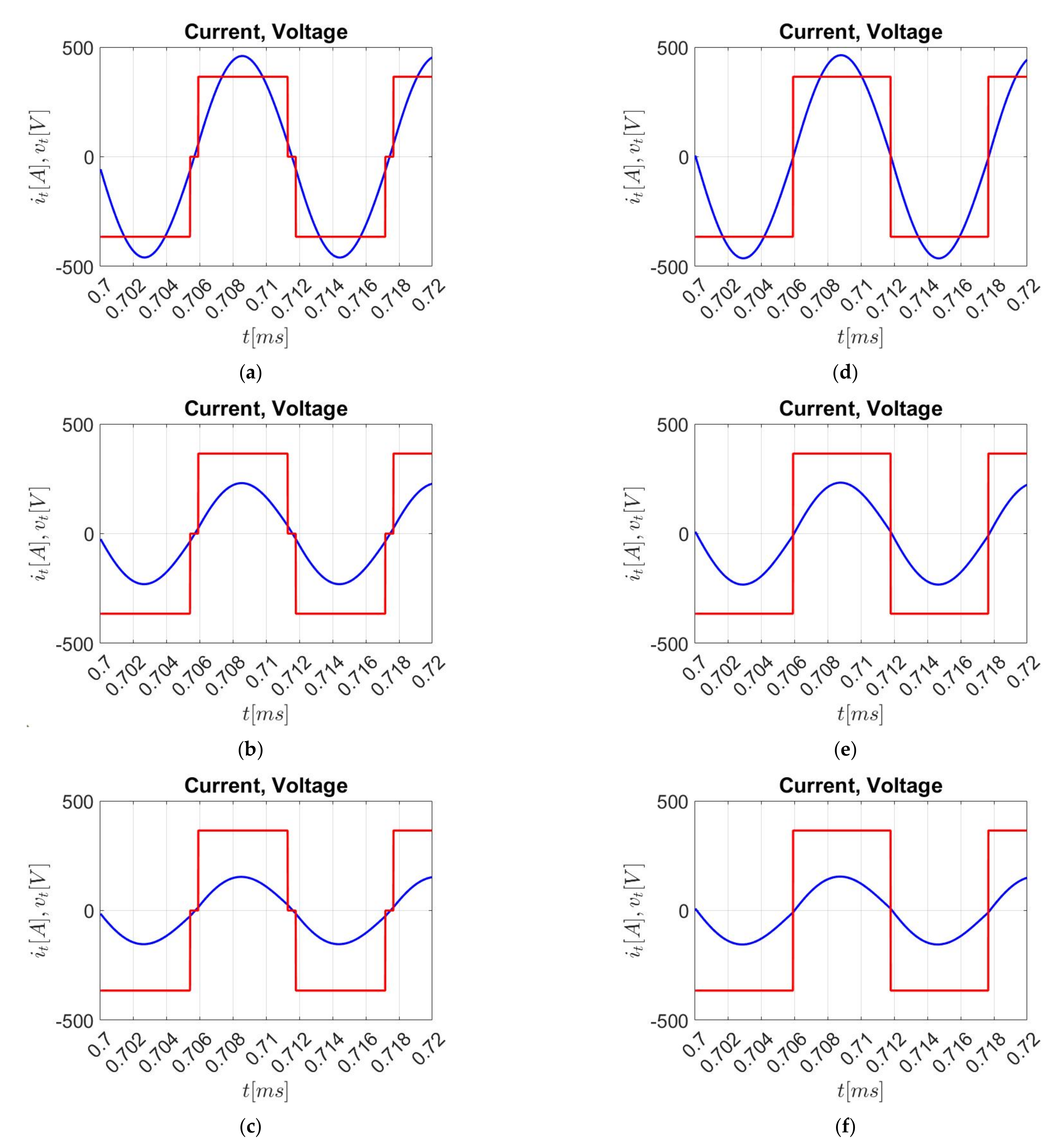
αP	Perturbations angle	45°, 60°

. To corroborate the hypotheses made in the previous sections, firstly, the steady-state waveforms have been captured and shown in Figure 5a–f with two small perturbations at secondary load, i.e., receiver side-reflected resistances to the transmitter side R are 5 Ω, 10 Ω, and 15 Ω, respectively. Here, it is observed that although the inverter output voltage contains several harmonics, the current i_t is nearly sinusoidal. This means that the resonant tank is very selective and filters all of the harmonics except the fundamental one. The assumption made in Figure 3 of considering the inverter as a sinusoidal voltage source corresponding to the fundamental of the inverter output voltage is then verified. In Figure 5, it is also shown that at steady-state, the current i_t is in phase with the fundamental of the inverter output voltage, which means that the inverter switching frequency is perfectly tuned to the natural frequency of the L_tC_t circuit, i.e., the angle ${\varphi }_{\mathrm{i}}$ in (9) is zero. A MATLAB scope acquisition of the current and voltage wave forms has been evaluated with the three different loads set to 5 Ω, 10 Ω, and 15 Ω, with a small perturbation angle of αP = 45° in time interval 0.7–0.72 ms, as represented in Figure 5a–c, respectively. It is verified, through the voltage waveform, that the conduction angle of the converter output voltage is greater than α = 120° due to the addition of the perturbation angle. Additionally, the fundamental voltage of the converter output voltage also increases. For further demonstration, the simulation result of the current and voltage wave form with perturbation angle αP = 60° is shown in Figure 5d–f, where the voltage wave form for the full half-cycle is depicted.

To verify the dynamic model, a small perturbation to the system has been introduced. The inverter phase-shift angle α, which was initially set to 120°, is increased by 45°. Accordingly, the fundamental of the inverter output voltage has been also increased. Indeed, its amplitude started from a value of $V_s=\frac{4}{\mathsf{\pi }}{V}_{DC}sin\left(\frac{{\alpha }_i}{2}\right)=402.5 \mathrm{V}$ and has reached an approximate value of 460.5 V. A MATLAB scope acquisition of the current has been triggered by the step change in α at 0.5 ms. The acquired current is one that flows through the H-bridge inverter output of the current i_t, and thus they share the same positive envelope. Then, inverter current waveforms with small perturbations of phase shift angle α, with the three different loads set to 5 Ω, 10 Ω, and 15 Ω are shown in Figure 6a–c. The transfer function (14) has been implemented in Simulink. Since it places the envelopes in relation, a voltage step of 58 V (corresponding to a step of 45° in α) has been provided as its input. The resulting output with the three loads set to 5 Ω, 10 Ω, and 15 Ω., which is the small-signal envelope of inverter output current, has been superposed on the steady-state value of the amplitude of the current i that is around 80.5 A, 40.25 A, and 26.8 A, respectively. The total signal has been plotted in the three different graphs of the inverter output current as shown in Figure 6a–c. It can be noticed that the output of (14) matches very well with the real envelope of the inverter output current, thus validating the MVLT model. For further demonstration, the simulation was again carried out for α = 60°, where the sinusoidal and the envelope matched properly. The plots are shown in Figure 6d–f.

6. Conclusions

In this paper, the novel MVLT method is explicated. The method is used to obtain the dynamic model of the resonant inverter that feeds the load of a WPT system. The discussion begins by obtaining the equivalent circuit model of the WPT system and underlining the hypotheses made for its derivation. It continues with the MVLT method description and its application to the considered resonant inverter. It has been demonstrated that the sought dynamic model can be obtained from the system original transfer function followed by a simple remapping in $s$-domain and a few additional mathematical steps. Unlike the existing GSSA and LPT methods, the MVLT technique emphasizes the link between the real signal transfer functions and the envelope transfer functions. Hence, the dynamic behavior of the envelopes can be directly assessed from the system transfer function. In this paper, the validity of the MVLT method has been verified by comparing the outcomes of the model implemented in Simulink. The result is satisfactory.