Abstract
Since battery electric vehicle (BEV) sales are increasing, the calculation of necessary electric power supply, and energy consumption data, and vehicle range is important. The Worldwide harmonized Light vehicles Test Procedure (WLTP) currently in use can deliver data to collect comparable energy consumption data for different vehicles on defined chassis dynamometer test cycles. Nevertheless, the energy consumption and so the range of BEVs are also dependent on the individual trajectory of the user. Therefore, five velocity profiles are developed in this work. The maximum speeds are based on typical velocities in German city traffic and extra-urban traffic. The energy required to finish a single velocity profile is assumed to be constant despite varying maximum velocities. With this kind of driving profiles it is possible to create an individual and more precise statement on the energy consumption and the range of a BEV. In this work, the profiles are driven on a chassis dynamometer with an VW e-Up. The vehicle charging efficiency is tested with two different AC charging modes and is also taken into account. The drive efficiencies of the tested vehicle are presented in dependence of the velocity profile driven. Finally the results are compared with a real-driving velocity profile and the energy consumption data obtained by the board computer of the vehicle.
1. Introduction
To determine the energy consumption of a vehicle, various driving cycles are used. The driving cycle developed by the European Union and introduced in the 1990’s is the new European drive cycle (NEDC). It was used to determine pollutant emissions, CO emissions and the fuel consumption of a vehicle. Thus, different vehicles could also be compared via the NEDC results. The duration of the cycle is 20 min, the maximum speed is 120 km/h and the average speed is 34 km/h. The NEDC has a stationary time share of 25%. Due to this proportion without vehicle motion, the large proportion of low speed and the maximum speed of only 120 km/h, this cycle was not corresponding well to the energy consumption under realistic conditions on roads. In order to provide the consumer with more realistic consumption data and to represent a more dynamic driving behavior of a vehicle, a new worldwide test procedure, the WLTC [1], was developed. The WLTP is a test procedure, that is intended to determine consumption, emissions and range on the basis of an objective and reproducible procedure. It is intended to reflect a real-world behavior in road traffic as accurately as possible. Thus, the WLTP’s driving cycle is more dynamic than the NEDC, has a much lower stationary portion of only 13% and a maximum speed of 130 km/h. In addition, the average speed is 46.6 km/h [1] and therefore higher than in the NEDC. The cycle is divided into four sections: low, medium, high and extra high. It is intended to represent different driving scenarios such as city traffic, extra-urban driving and highway driving. The average velocities of the different cycle components from low to extra high are 18.9 km/h, 38.5 km/h, 56.6 km/h and 92 km/h [2].
For battery electric vehicles, the specified range as well as the energy consumption per 100 km is calculated on the basis of the WLTP in Europe and the accuracy plays a very important role for BEVs as these parameters represent an important criterion in the selection of the vehicle to purchase [3]. The WLTP provides a more realistic test cycle in comparison to the NEDC. Still, in various publications it can be found that the energy consumption in reality deviates significantly from the data according to WLTP [4,5].
Reasons for this can be found in the individual driving behavior and also in external factors, such as the surrounding temperature [4].
Since none of the presented test cycles allow the computation of the energy consumption of an individual trajectory mix, new velocity profiles are proposed in this study. The proposed profiles are driven with a Volkswagen e-Up on a chassis dynamometer. With the velocity profiles it is possible to make a more realistic and individual statement about consumption and range. Thus, the individual driving profiles and their consumption can be individually weighted according to usage behavior. In addition, the different efficiencies of driving and charging will be investigated to identify reasons for increased consumption in certain areas.
The goal of this paper is to propose a simple chassis dynamometer test that is able to create an individual and precise statement on the energy consumption as well as the range of a BEV to predict the energy consumption in real-world driving based on a velocity profile mix. Five velocity profiles are proposed and developed in this work. The tests are performed on a chassis dynamometer at the Ravensburg-Weingarten University of applied sciences at ambient conditions. The profile data is matched to clustered real-driving velocity profile data. Finally the results from the dynamometer test are combined and compared with the real-driving velocity profile and the energy consumption data presented by the board computer of the vehicle. This qualifies the developed test for certain conditions. The real-driving tests are repeated, so that traffic and slight temperature change influences can be estimated.
Still, there are many influence factors like changing ambient temperatures which are not analyzed in detail in this investigation. A further target is the proof of concept concerning the testing procedure and calculation of consumed energy. In further investigations, the method can be refined, for example, to include the influence of the ambient temperature or battery aging. This study is intended to lay the foundation for subsequent research in this field.
2. Materials and Methods
This chapter describes the choice of velocity profiles. It also specifies the test vehicle and the exact measurement setup with all the measuring equipment used. Additionally a detailed description of the measurement procedure is provided. Furthermore, the formulas used for the subsequent calculation of the different efficiencies in the vehicle are presented.
2.1. Velocity Profiles
To support a partly individual driving profile, five different velocity profiles are proposed. They are based on common driven velocities on German roads. The defined maximum speeds are 35 km/h, 55 km/h, 85 km/h, 100 km/h and 130 km/h. All maximum speeds are reached with a constant acceleration of 0.8 m/s2. After a constant top speed, the vehicle is brought to a stop with a constant deceleration of m/s2. All velocity profiles are designed to consume the same amount of energy. For the VW e-Up as an example, this energy is 298.9 Wh for all velocity profiles and is calculated using formula (3). The energy content of the profiles is calculated via the driving resistance and is individual for each tested vehicle. The considered resistances are rolling resistance , air drag and the inertial resistance , given in Equation (1). The data used for the calculation of the driving resistance is listed in Table 1.

Table 1.
Parameters for calculating the driving resistances of the VW e-Up.
The presented data from Table 1 is also used by the dynamometer control so simulate inertia and air drag losses. During the constant deceleration phase, regeneration is allowed. The VW e-Up tested is not able to achieve a constant deceleration of m/s2 through recuperation alone. Additional energy is converted into heat in the mechanical brake to achieve this. A vehicle that can decelerate as requested with recuperation only will achieve better efficiency values in this test.
The overall driving resistance can be calculated employing Equation (1).
The overall driving resistance is used to calculate the power for each speed along the velocity profile with, given in Equation (2).
The energy content of the complete velocity profile is calculated by integrating the calculated resistance power , see Equation (3).
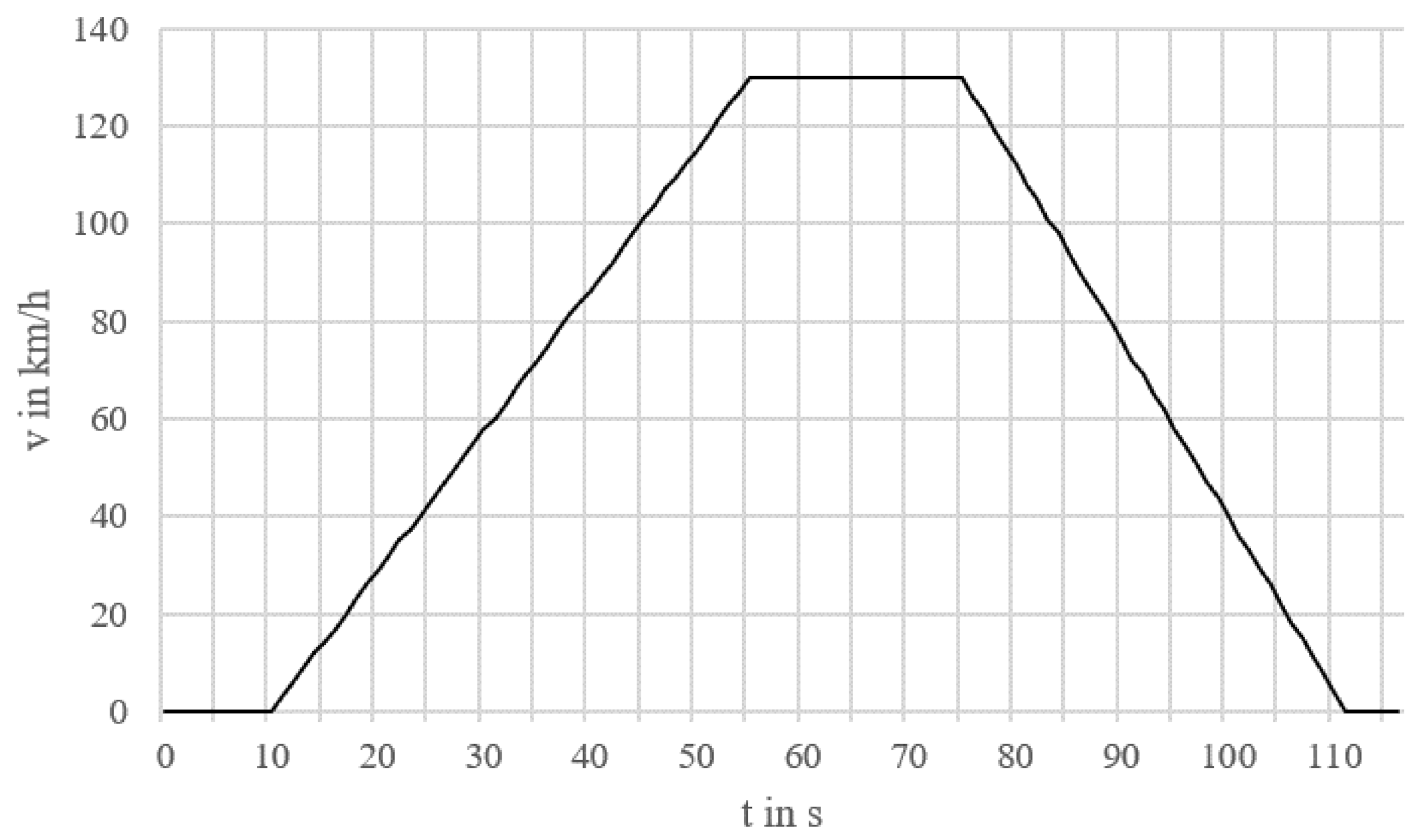
A constant required energy demand is achieved by holding the maximum speed for different lengths of time, as the resistance power is increasing with higher velocities. For the 35 km/h profile, the maximum speed is thus held for significantly longer than for the 130 km/h profile. The 130 km/h velocity v profile in km/h is shown in Figure 1 over the time t.
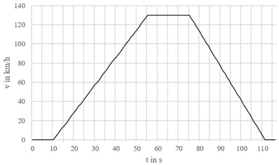
Figure 1.
Example velocity profile with maximum speed 130 km/h.
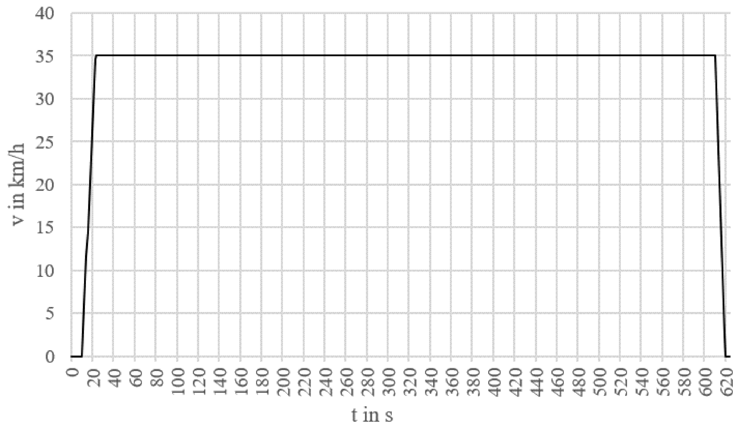
Figure 2 shows the 35 km/h profile over the time t. As described, the initial acceleration and braking deceleration is of the same magnitude for both presented profiles. A comparison of the two presented profiles shows the difference in the duration of the maximum speed held constant.
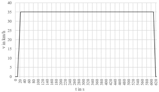
Figure 2.
35 km/h speed profile.
2.2. Test Vehicle
The test vehicle is a Volkswagen e-Up (model year 2019). It is a battery electric compact car. Table 2 shows the important technical data like the battery net energy, the maximal charging power, the WLTP range and also the WLTP energy consumption given by the OEM [6].
Table 2.
Relevant vehicle data.
2.3. Measurement Setup
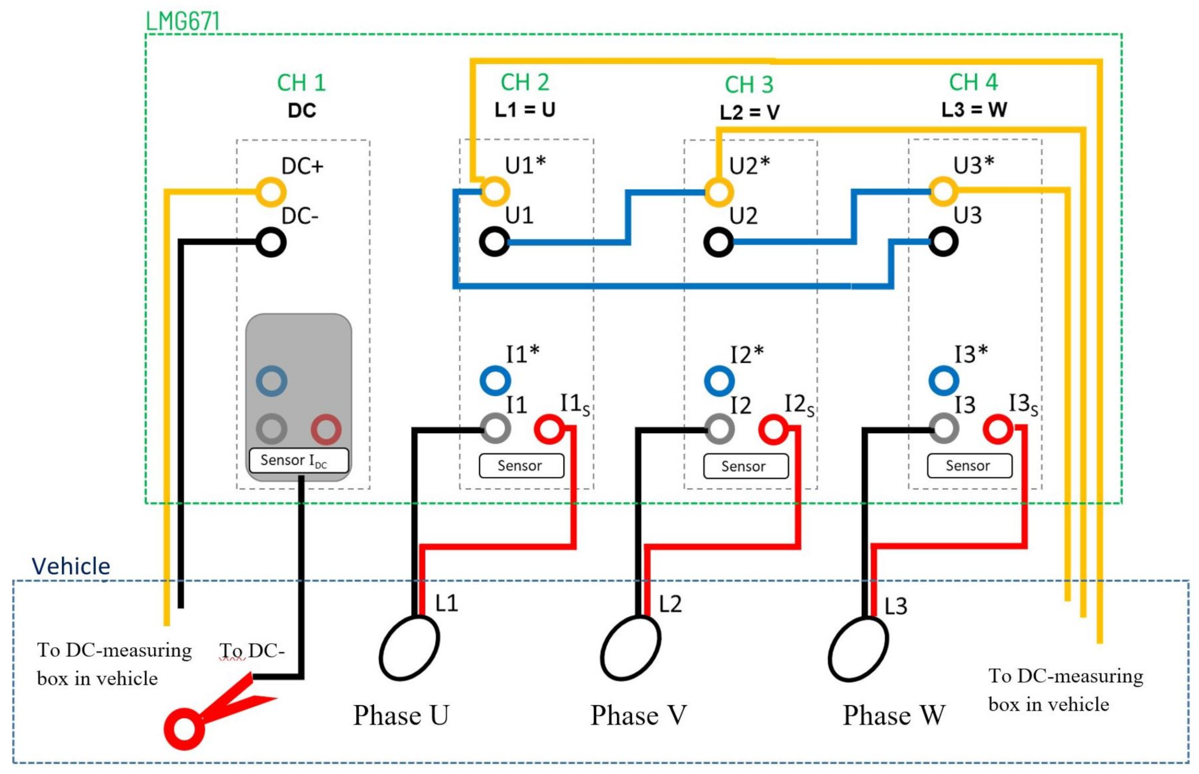
For the modeled test method, two different measurement setups are used. The first measurement setup enables a measurement while undergoing one of the velocity profiles on the dynamometer. In this study, the vehicle is mounted on a MAHA apex chassis dynamometer (MSR500) at the RWU. The dyno records the wheel force and velocity [7]. In addition, a Zimmer LMG671 power meter is used to measure the voltages on the AC and DC circuits of the vehicle direct. This is enabled by modifications to the high-voltage wiring of the VW e-Up. The DC current is measured indirect with a current clamps. On the AC side, the current is measured with Rogowski coils. Figure 3 shows the LMG671 is connections to the vehicle. The illustration shows the LMG671 backside interface on the top of the figure. Four measurement channels are used (CH1, CH2, CH3 and CH4). All channels offer two voltage measurement input plugs on the top side of each channel and three current measurement inputs on the bottom of each channel. There are three inputs because one is used for indirect current measurements by a voltage measurement. The other input labeled with a star (*) are for direct current measurements up to 15 amperes and is thus not useful for this experiment. Voltage and current are recorded synchronously in time by the power meter. An electrical effective power is calculated directly from the power meter (AC and DC). According to Equation (3) an electric energy is calculated from the electrical effective power via integration in a post process. The calculated electrical power and energy is used to calculate the efficiencies in this study.
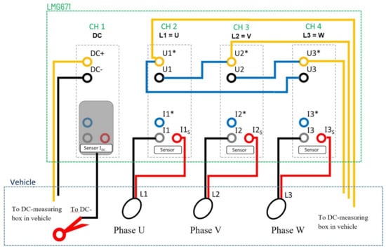
Figure 3.
Schematic connections of the LMG671 and the vehicle.
CH1 is connected to the DC circuit of the vehicle on the output side of the power electronics and measures the energy flux from the battery to the power electronics or vice versa. The yellow and black connections labeled with DC+ and DC- are voltage measurements, the black connection on the bottom side of the LMG671 CH1 is connected to the illustrated current clamp, mounted on the DC- side.
CH2 to CH4 are connected to the AC circuit of the vehicle. The energy that is flowing from the DC circuit of the vehicle to the electric machine is measured by the red and black connections illustrated and connected with the Rogowski coils. The three phases of the vehicles’ electric engine are labeled with U, V and W or L1, L2 and L3. The yellow lines are directly connected to the three phases and connected so that the voltage of each phase can be determined.
The measured currents and voltages are used to calculate the electric power between the power electronics and the electric engine and the power between the power electronics and the high-voltage battery. In analogy to the setup of CH1 illustrated in Figure 3, the current and voltage of the 12 V low-voltage system is measured on channel 5 (CH5) of the LMG671 to calculate the power consumption of the 12 V on-board power supply . This is important as the DC/DC (high voltage > 60 V to low voltage ≤ 12 V) converter may charge the 12 V battery during the testing. This energy has to be taken into account for the computation of the energy balance.
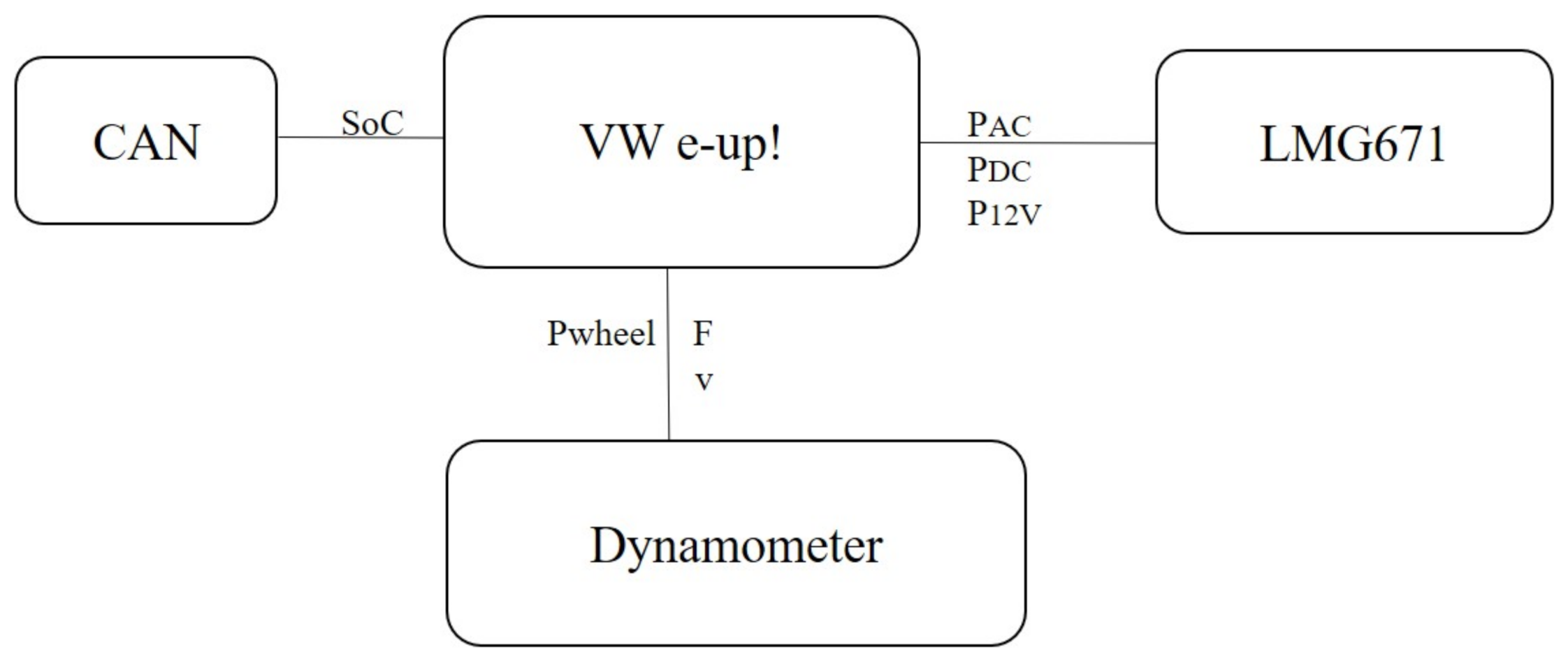
The CAN-data of the VW e-Up is recorded while driving. The overal measurement setup 1 is shown schematically in Figure 4. As described the LMG671 is connected to the vehicle and measures voltages and currents which enable the calculation of , and . The only necessary quantity from the CAN-bus is the state of charge (SoC) from the e-Up battery management system. The dynamometer provides the wheel force F and the dynamometer roller velocity v which is assumed to be the vehicle velocity. So for this test setup wheel slip is neglected as driving power levels are low, this is valid. With this information, a wheel power can be calculated using F and v.
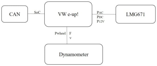
Figure 4.
Schematic illustration of the overal measurement setup for driving.
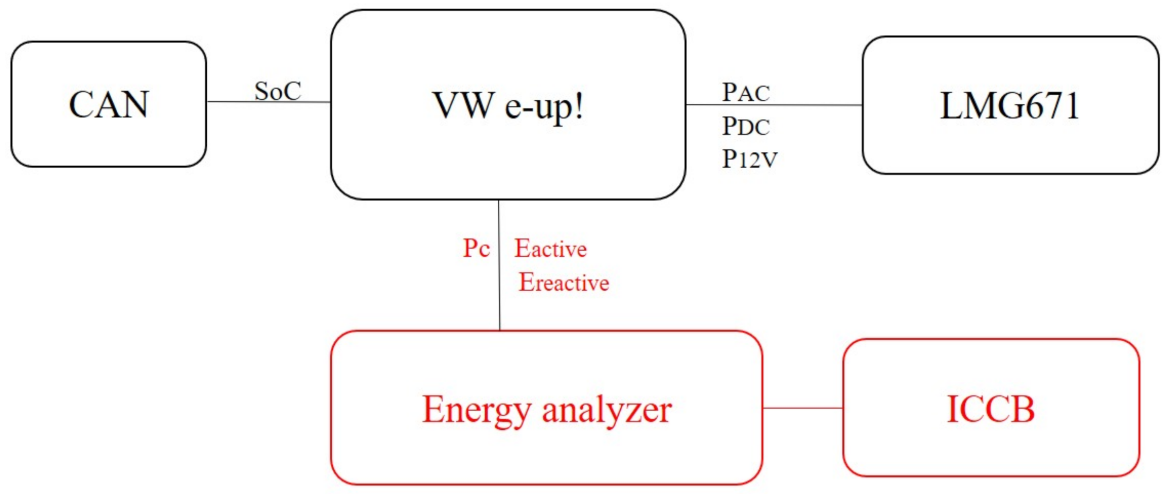
The second measurement setup is used for the subsequent charging process. Here, in analogy to the measurement setup for driving, the power meter is also connected to the vehicles AC and DC circuits. Again the resulting powers , and are calculated. In addition to the power meter, a self developed energy energy analyzer is connected between the wallbox which is used for BEV charging and the type 2 charging plug of the vehicle. This energy analyzer records the charged energy over time. It also calculates active and reactive energy. The thesis from Bannholzer describes the structure of a energy analyzer with the same measurement principle in detail, see [8]. The difference to the energy analyzer described in [8] is, that the one used for this study has a type 2 input and thus the wallbox, in this case a juice booster portable wallbox, is connected directly to the energy analyzer. The vehicle is also connected with a type 2 plug to the energy analyzer. The overall measurement setup for charging is shown in Figure 5.
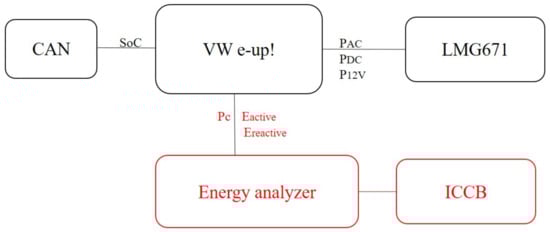
Figure 5.
Schematic illustration of the overall measurement setup for charging.
2.4. Measurements
The procedure for an overall measurement as proposed in this paper is as follows. The starting point for each individual test component is a fully charged vehicle battery. Each velocity profile is completed on the test bench with the described measurement setup for driving. Then the consumed energy content is measured in the measurement setup for charging at maximum AC charging power. In this way, the efficiency and the actual consumed energy content of each profile can be determined. All controllable additional consumers in the 12 V board network, as the radio and air conditioning, are switched off while driving.
In addition, two full charging processes were recorded to identify differences in the charging efficiency at different charging powers. For this purpose, the vehicle battery was emptied twice and then recharged once with maximum AC charging power, which in this case corresponds to 16 A and 7.3 kW two-phase charging, and once with the in cabel control box (ICCB) at the household socket single-phase charging with a 10 A current. The SoC of the gross energy content of the battery was extracted via the CAN interface before and after each charging stroke. Furthermore, the power flow of the 12 V battery was calculated with the measured voltages and currents from the power meter.
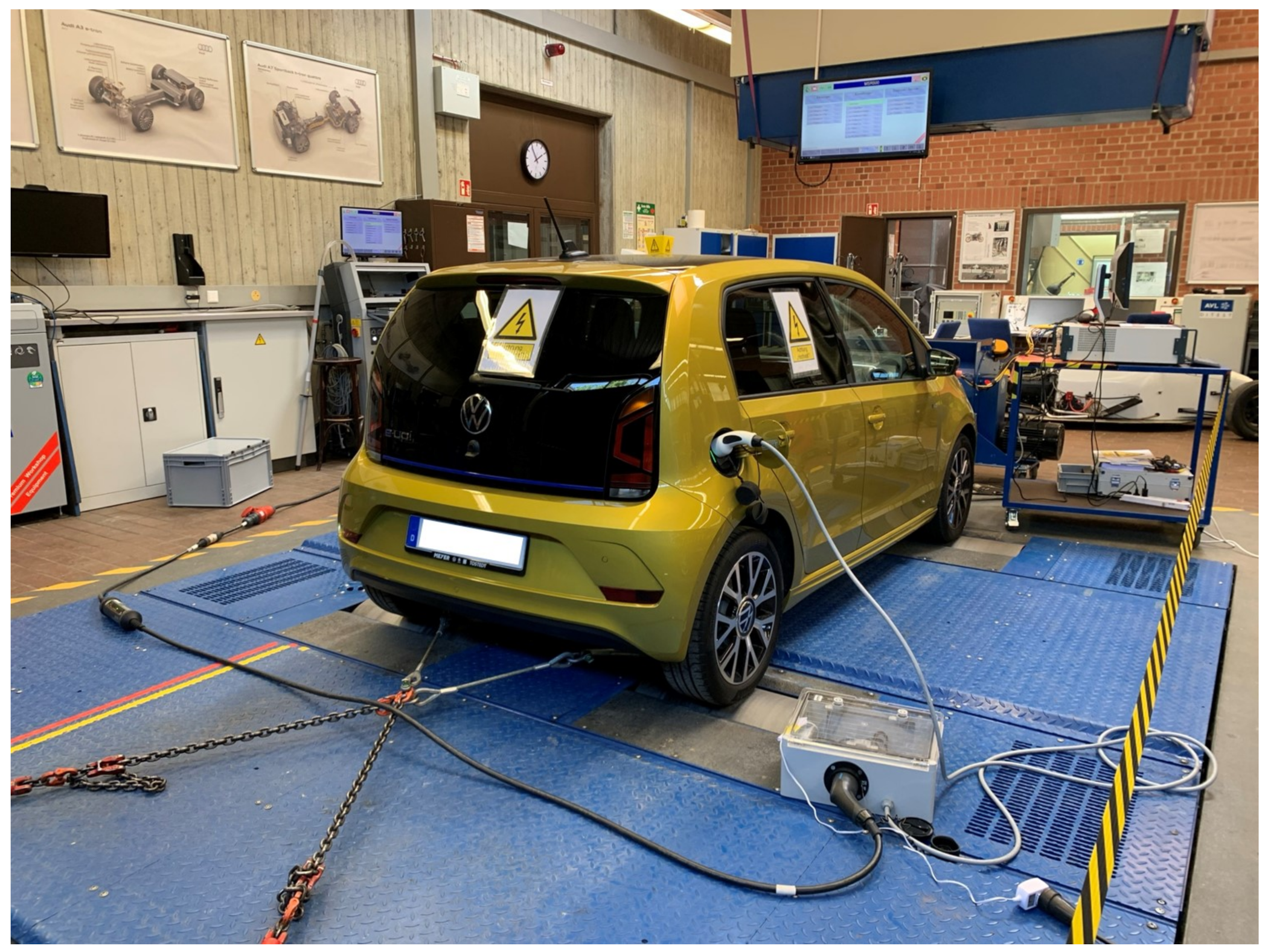
Figure 6 shows the tested VW e-Up on the MAHA MSR500 chassis dynamometer with the portable wallbox as well as with the developed energy analyzer plugged to the vehicle. In the front of the car the LMG671 is connected to the vehicle. The picture was taken during a charge process.

Figure 6.
VW e-Up on the test bench connected with the energy analyzer and the LMG67184.
The measurement accuracies specified by the manufacturer of all measurement devices used for the tests are presented in Table 3.
Table 3.
Accuracy of the individual measuring devices.
2.5. Efficiency Calculation
The charging efficiency is calculated using the determined charging power in the developed energy analyzer as input power and from the LMG671 as output power from the on-board charger of the vehicle. This method has the advantage that it uses external measurement equipment and therefore does not rely on CAN-bus data or manufacturer specifications with unknown accuracy.
In addition, the charging efficiency for both charging modes are calculated in another way. The quantities used are the gross energy content provided by Volkswagen, the active energy measured by the developed energy analyzer and the and , determined via the CAN-bus before and after charging the vehicle.
The efficiency of the drivetrain is calculated using the resulting energy, converted into heat by the eddy current brakes of the chassis dynamometer during the respective driving profile. This energy is defined as the output energy and it is computed by the dynamometer based on a time, force and speed measurement. The energy flowing from the DC circuit of the vehicle to the electric machine, which is measured by the power meter LMG671 is defined as input energy.
The relevant overall efficiency of the vehicle from the charging socket to the wheel is calculated from the efficiency of the drivetrain and the averaged charging efficiency for a total charging stroke. In the present case, the charging power and also the charging efficiency of the vehicle varies during a full charging stroke. For the vehicle user, it therefore makes a difference whether the vehicle is fully charged starting from a low SoC or from a high SoC. To eliminate this influence, the averaged efficiency of a full charge stroke is calculated in (7) with :
3. Results
The aim of the measurements is to compare the consumption of different velocities, as well as to see driving and charging efficiencies. In addition, two different charging modes are compared.
3.1. Energy Consumption
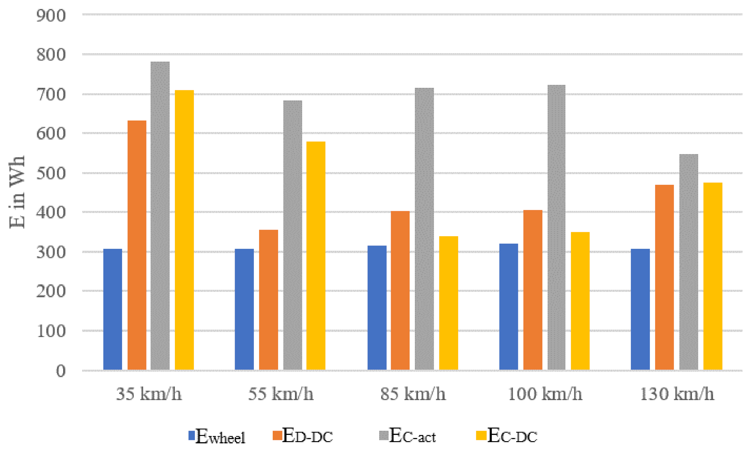
In this section, the energy consumption at the different measuring positions are described and compared, see Figure 7.

Figure 7.
Energy consumptions of all driving profiles.
describes the energy absorbed by the eddy current brakes of the chassis dynamometer. Figure 7 shows this energy colored in blue for the different velocity profiles. The deviations between the different tests should be very small and close to 300 Wh (298.9 Wh calculated). This ensures that the same energy content is converted in each profile. The maximum deviation in the measurement series shown to the calculated value is 7.73%, which results from a manual driving on the dynamometer and could be improved by more practice or a driving robot.
is the DC-circuit energy put into the electric motor while driving. In Figure 7 it is shown that the energy needed for a particular velocity profile differs by each maximum speed. It is the highest in the low speed profile with a maximum speed of 35 km/h and the lowest for 55 km/h. For 85 and 100 km/h the energy consumed is 440 Wh. At a maximum speed of 130 km/h the energy needed is 510 Wh.
is the charged active energy amount measured with the developed energy analyzer after the respective driving profile. is the charged energy amount measured by the power meter on the DC-circuit during each charging process. As Figure 7 shows, it seems that there is no correlation between the measured energies. Therefore, further research was conducted on this behavior by analyzing the 12 V energy data.
Because the behavior of the individual systems, e.g., the battery management system, cannot be analyzed in detail, the following causes for the deviations shown are possible:
- The energy consumption by control units in the 12 V system varies.
- The 12 V battery is recharged while charging the high-voltage battery. The maximal energy stored in the 12 V battery is around 480 Wh which can cause large deviations between and .
- The cells of the high voltage battery are balanced by the battery management system (BMS). This amount may differ each charging process and as the BMS behaviour is a black-box the energy amount is not traceable.
- Since the vehicle stops the charging process itself and the SoC may not be precise, it may be that the BMS stops the charging process at different capacity levels.
- The external and battery temperature, voltage recovery after load drop as well as battery aging may play also a role.
Due to this phenomenon, it is more meaningful to measure the charging efficiency over almost full charging strokes rather than after completing the speed profiles. The determination of a charging efficiency at a low energy extraction as in the present case would lead to large errors (up to 50% or more) due to the causes mentioned.
3.2. Charging Efficiency
As described in Section 3.1, as close as possible total charging strokes are recorded to determine a mean charging efficiency. This chapter presents the charging efficiency purely based on external measurements and the charging efficiency which is based on the battery gross energy as specified by VW and the vehicle CAN-bus SoC data. The results of this efficiency data is presented for two measured charging strokes in Table 4.
Table 4.
Charging strokes.
In the first charging stroke, the maximum AC charging power of the on-board charger was used, which corresponds to 7.3 kW, 2 phases used and 16 A (2P16A). The battery start SoC is 13.725% and the battery is then charged until the vehicle stops the charging operation. An end SoC of 94.117% is achieved. The charged energy in this case is 35.03 kWh. The second charging stroke is performed with the ICCB at a household socket. Charging is performed with one phase and 10 A. This results in a maximum charging power of 2.3 kW. Here, the vehicle’s battery start SoC is 12.16% and then end SoC is again 94.117%. An energy of 36.74 kWh was recharged. Since the SoC CAN-bus data does not exceed 94.117% this is the SoC referring to the gross battery capacity.
As described in Section 2.5, the charging efficiency is calculated in two ways. As shown in Table 4 the results from the two calculation methods presented differ. One reason may lie in inaccuracies of the CAN-bus SoC data. For example, assuming the end SoC value to be 100% instead of the 94.117% results in charge efficiencies of 90.6% (2P16A) and 87.98% (1P10A). These are already significantly closer to the calculated efficiencies which were recorded using accurate external measuring equipment. Moreover, these values correlate better with the determined efficiencies in known publications, see [2,5,9].
For this reason, the efficiency according to is used for further considerations, which results in 92.66% for 2-phase charging with 16A and 86.79% for 1-phase charging with 10 A.
3.3. Drivetrain Efficiency
The drivetrain efficiency calculation is described in Section 2.3 in detail. Table 5 shows the resulting efficiencies for each velocity profile. The drivetrain shows the worst efficiency with 48.5% in the profile with 35 km/h maximum speed. At low vehicle speeds, the efficiencies in the electric machine are low due to ohmic losses. In the mechanical drive train the efficiency is low due to a relatively high proportion of frictional losses. The best efficiency is achieved with the 55 km/h profile and is 86.86%. At a maximum velocity of 130 km/h the efficiency is significantly lower than for a maximum profile velocity of 100 km/h or 85 km/h.
Table 5.
Drivetrain efficiency data.
3.4. Total Efficiency
Table 6 shows the total efficiency of the vehicle in all tested velocity profiles. The total efficiency includes the drivetrain and the charging efficiency. The total efficiency is calculated with the calculated mean charging efficiency from Table 4 with 2 phases and 16 A.
Table 6.
Total efficiency for each velocity profile.
This procedure changes only the absolute values compared to the data from Table 5. The relative gradation of the efficiency values is preserved.
The overall efficiency is dominated by the drivetrain efficiency and the charging efficiency only plays a minor role.
3.5. Energy Consumptions Per 100 km
To represent the vehicle consumption per 100 km for each profile, the total energy consumption is calculated using the total efficiency and the energy absorbed by the rollers of the chassis dynamometer. In addition, the velocity data from the chassis dynamometer can be used to determine the distance traveled in each tested profile. Table 7 presents this data and the energy consumption per 100 km. For a maximum velocity of 130 km/h, the consumption is the largest with 23.94 kWh/100 km. The lowest energy consumption of 8.35 kWh/100 km is found in the 55 km/h profile. This is due to the excellent efficiency of the drivetrain at this velocity.
Table 7.
Distance traveled and energy consumption per 100 km.
3.6. Application on Real-Driving Velocity Profiles and Comparison of the Resulting Energy Consumption
The speed-dependent energy consumption data can be applied to clustered speed data from real-driving profiles. Figure 8 presents clustered data from a route including city driving, interurban driving and expressways. The route from Radolfzell (Lake Constance) to Weingarten in Baden-Württemberg Germany is 86 km long. The route was driven with summer tires at about 25 °C outdoor temperature. This temperature is close to the ambient temperatures during the passed chassis dynamometer tests. Velocities lower than 70 km/h do have a share of more than 60% of the overall time. More than 14% of the time, the velocity was larger than 92.5 km/h.
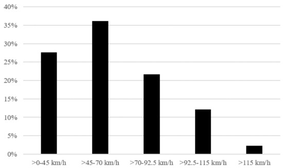
Figure 8.
Percentage share of different velocities for an example route.
The velocities are clustered into five ranges over time. Range 1 is the share of velocities to 45 km/h, range 2 sums up the speed data between 45 km/h and 70 km/h, range 3 from 70 km/h to 92.5 km/h, range 4 from 92.5 km/h to 115 km/h and range 5 includes all velocities larger than 115 km/h. By multiplying the resulting percentages of the clustered data with the consumption data per 100 km from Table 7 an average consumption of 11.69 kWh per 100 km results.
The vehicle display indicated a energy consumption of 10.8 kWh/100 km on the presented route. The route is also driven several times at similar temperatures to break down the daily influence of slightly varying temperatures and traffic. The energy consumption given by the vehicle lies between 9.8 kWh/100 km and 12.9 kWh/100 km. The presented energy consumption by the board computer does not take into account the charging efficiency. A division of the charging efficiency (92.66% at 2P16A) of the presented 10.8 kWh/100 km results in a total energy consumption of 11.66 kWh/100 km.
The result is already very close to the 11.85 kWh/100 km obtained on the chassis dynamometer using the presented velocity profiles. This results in a low deviation between the chassis dynamometer data and the real-driving profile of 1.6%. The maximum deviation of the chassis dynamometer data and the presented real-driving energy consumption data range is 26.16% (82.7% up to 108.86%).
4. Discussion and Outlook
The large charge strokes show that there is a difference of 5.87% in the charging efficiency between charging with only one phase and 10 A (ICCB) and charging with the maximum AC power (2 phases, 16 A). Thus, the charging efficiency at the maximum charging power is 92.66%. If charged with the ICCB the charging efficiency is only 86.79%. A comparable behavior can be observed in [2] from charging efficiency data of a KIA e-Niro.
The efficiency of the drivetrain and thus the total efficiency are dependent on the velocity driven, as can also be seen in the performed tests. The efficiency of the drivetrain is 48.5% in the 35 km/h profile. The best efficiency is achieved with the 55 km/h profile and is 86.86%. In the 85 km/h and 100 km/h profiles, is very close with 77.97% and 79.50%. With 60.43%, the vehicle has a lower efficiency in the 130 km/h profile. Since the test vehicle is a Volkswagen e-Up and is designed for city driving, it is plausible that the drivetrain has the best efficiency in the 55 km/h profile.
Thus, the consumption per 100 km is the highest with the 130 km/h profile, which is amplified due to the increased air resistance at high velocities.The vehicle has the lowest consumption per 100 km in the 55 km/h profile, due to the high drivetrain efficiency in this velocity range, the consumption is even lower than at the 35 km/h profile.
Through the division into the 5 velocity profiles, it is possible to make more individual statements about the energy consumption and the range of the vehicle. Depending on the driving behavior, the profiles can be calculated proportionally. The study compares a real-driving speed profile with the data collected in the dynamometer tests. Speed range time shares of the real-driving route are clustered and the energy consumption is read out from the board computer of the vehicle. The time shares are then multiplied with the energy consumption test data per 100 km. The results show that in the best case an accuracy of 1.6% can be achieved. In dependence of slightly varying temperatures and various traffic conditions the results still only deviate from the ideal case by a maximum of 26.16%. However, it must be taken into account that no new calculation of the velocity time shares was performed for the other consumption data given as range (9.8 kWh/100 km to 12.9 kWh/100 km). The accuracy with a recalculation of the time shares will improve this result significantly.
Test data as presented in this study provide the user with more precise and individual information and lead to plausible real world consumption prediction. The charging mode used can be taken into account, as it plays a significant role in the total efficiency of the vehicle and in the costs and the CO-emissions. The tests do not take into account that stop and go occurs more frequently in city traffic than in higher velocity ranges on highways and that the consumption can be strongly affected by this. Also the energy consumption is higher at low outdoor temperatures and with winter tires.
In general, the battery temperature plays a major role in terms of a vehicles’ energy consumption. This temperature can deviate from the ambient temperature and thus the internal resistance of the battery also changes independent from ambient conditions and should also be considered in future studies.
In charging operation the behavior of the battery management system is a black-box. It is therefore recommended to record at least two charging strokes for each charging mode in order to be able to make a more accurate statement about the charging efficiency. Furthermore, the capacity in ampere hours (Ah) can be used as a comparative value because the voltage of the vehicle is subject to further dependencies. For example, the voltage needs some time to recover to a constant level after a high battery load. In this way, the charging efficiency can be determined more accurately and independently of the voltage.
Author Contributions
Conceptualization and methodology, A.K. (Anja Konzept), B.R., A.K. (André Kaufmann), R.H. and R.S.; development measurement technology, A.K. (André Kaufmann) and R.H.; measurements, A.K. (Anja Konzept), B.R., A.K. (André Kaufmann) and R.H.; measurement result evaluation, A.K. (Anja Konzept), B.R. and A.K. (André Kaufmann); high voltage safety responsibility, R.H.; writing—original draft preparation, A.K. (Anja Konzept); writing—review and editing, B.R., A.K. (André Kaufmann) and R.S. All authors have read and agreed to the published version of the manuscript.
Funding
This research received no external funding.
Institutional Review Board Statement
Not applicable.
Informed Consent Statement
Not applicable.
Conflicts of Interest
The authors declare no conflict of interest.
Abbreviations
The following abbreviations are used in this manuscript:
| AC | Alternating Current |
| BEV | Battery electric vehicle |
| BMS | Battery management system |
| DC | Direct current |
| ICCB | In-cable control box |
| NEDC | New European Driving Cycle |
| WLTP | Worldwide harmonized Light vehicles Test Procedure |
| 2P16A | 2 phases and 16 A |
| 1P10A | 1 phase and 10 A |
References
- NEFZ und WLTP. Available online: https://en.vda.de/de/themen/umwelt-und-klima/nefz-und-wltp/nefz-und-wltp.html (accessed on 10 November 2021).
- Reick, B.; Konzept, A.; Kaufmann, A.; Stetter, R.; Engelmann, D. Influence of Charging Losses on Energy Consumption and CO2 Emissions of Battery-Electric Vehicles. Vehicles 2021, 3, 43. [Google Scholar] [CrossRef]
- Rachel, L.; Daniel, K.; Tim, J.; Gretchen, M. Ease of EVs: Exploring factors that influence battery consumption. Int. J. Sustain. Transp. 2020, 14, 701–709. [Google Scholar] [CrossRef]
- Kamguia Simeu, S.; Brokate, J.; Stephens, T.; Rousseau, A. Factors Influencing Energy Consumption and Cost-Competiveness of Plug-in Electric Vehicles. World Electr. Veh. J. 2018, 9, 23. [Google Scholar] [CrossRef] [Green Version]
- Stromverbrauch Elektroautos: Aktuelle Modelle im ADAC Test. Available online: https://www.adac.de/rund-ums-fahrzeug/tests/elektromobilitaet/stromverbrauch-elektroautos-adac-test/ (accessed on 10 November 2021).
- Sonderangebot mit Liefer-Engpass: Der VW e-Up im ADAC Test. Available online: https://www.adac.de/rund-ums-fahrzeug/autokatalog/marken-modelle/vw/vw-e-Up/ (accessed on 10 November 2021).
- Reick, B.; Kaufmann, A.; Engelmann, D. Test Procedure Proposal for EV Power Measurement on Dynamometers. In Proceedings of the International Conference on Vehicles and Engines, Capri, Italy, 13–15 September 2021. [Google Scholar] [CrossRef]
- Bannholzer, F.; Engelmann, D. Entwicklung einer Messbox für die Aufzeichnung von Energieverbrauch und Ladeleistung während des Ladevorgangs eines E-Fahrzeuges. Bachelor’s Thesis, Berner Fachhochschule, Biel, Swizerland, 2021. [Google Scholar]
- Apostolaki-Oisifidou, E.; Codani, P.; Kempton, W. Measurement of power loss during electric vehicle charging and discharging. Energy 2017, 127, 730–742. [Google Scholar] [CrossRef]

Publisher’s Note: MDPI stays neutral with regard to jurisdictional claims in published maps and institutional affiliations. |
© 2022 by the authors. Licensee MDPI, Basel, Switzerland. This article is an open access article distributed under the terms and conditions of the Creative Commons Attribution (CC BY) license (https://creativecommons.org/licenses/by/4.0/).