Wireless Power Transfer System in Dynamic Conditions: A Field-Circuit Analysis

Abstract

In the paper, a Finite Element (FE) Analysis for investigating the electric properties of a Wireless Power Transfer System (WPTS) devoted to charging the batteries of electric vehicles is performed. In particular, the dynamic-WPTS, which is challenging because of the position-varying properties of the system, is considered. The field analysis is computationally heavy because of thin conductive layers modelling the car chassis: an effective analytical approximation for the field calculation in thin layers is applied to both the car frame bottom and the shielding aluminum layer. This approach allows for an accurate solution and, meanwhile, for a reduction in the computational costs, making the repeated simulations feasible.

1. Introduction

Wireless Power Transfer (WPT) is an emerging technology to charge the onboard batteries of an electric vehicle (EVs) using magnetic induction instead of classic plug-in battery chargers [1,2,3,4]. The simplest WPT systems (WPTSs) are based on a pair of coils, a transmitting and a receiving one, separated by an air gap [5]. In general, the transmitting coil is buried under a parking pitch while the receiving coil is mounted under the chassis of the vehicle and the onboard battery is charged while the car is parked. In this case of static recharge, a careful positioning of the vehicle on the parking pitch assures a good alignment between the coils and the maximum mutual inductance [6]. Much more challenging is the design of the dynamic WPTSs, which are devoted to charging the battery while the vehicle runs over suitable roads, denoted as tracks, equipped with a set of transmitting coils fitted below the road surface. In the case of dynamic WPTSs, the receiving coil subsequently experiences full-alignment, partial alignment and no-alignment conditions. Then, it could be reasonable to investigate the variation of magnetic field, and so self- and mutual inductance considering different scenarios from the fully aligned to the completely misaligned coils [1,7,8]. Specifically, the FEA evaluates the lumped parameters related to the self- and mutual-inductance of the WPTS device as a function of the alignment of the receiving and transmitting coil.

In the paper, the pair of coils is simulated in a sequence of Finite Element Analyses (FEA) considering the receiving coil at different fixed positions with respect to the transmitting coil. Dynamic WPTSs are characterized by a number of transmitting coils deployed along the track [1]; in the paper, the distance between them is considered to be long enough to make negligible their mutual inductances to allow the receiving coil to be coupled with only one transmitting coil at a time.

Together with the receiving coil, a simplified model of the bottom of the chassis is considered in the FEA. It includes three layers: the steel car frame bottom (mechanical structure), an aluminum plate (eddy current shield) and a ferrite core (magnetic field concentrator). The following scenario will be considered: both the car and the track are equipped with circular coils [9].

Following the SAE standard, the transmitting coil is supplied by current at 85 kHz. The FEA considers the coupling coils of the small size WPTS experimented in [7]. The prototype is sized to transfer a power of 600 W onboard a minicar to charge its battery. At nominal condition the current in the transmitting coil is 5.7 A and the corresponding voltage induced across the receiving coil is about 90 V.

The paper is organized as follows: in Section 2, the analysis problem is described; in Section 3, the results are presented, and finally, a conclusion is drawn.

2. Analysis Problem

A 3D Finite-Element Model (FEM) of the transmitting-receiving coils is developed here and used to extract lumped parameters in terms of the mutual inductance vs. relative position curve [10,11,12]. To this end, the vehicle frame is modeled as a simple steel sheet, 800 mm width, 800 mm deep (actually, 400 mm in the model exploiting symmetry) and 0.7 mm thick. The rationale is the following: even if it is a simplified model of a real chassis, the discretization of a device exhibiting very different geometric dimensions, as well as the requirement of generating mesh elements the dimensions of which depend on the penetration depth of the eddy current (that is in the range of some micrometers), might lead to a very large number of elements and high computational cost. Between the vehicle frame and the ferrite layer of the receiving coil an aluminum sheet, 600 mm width, 600 mm deep, 0.76 mm thick is introduced in order to shield the magnetic field and to reduce eddy current in the magnetic steel representing the car frame. For this twofold reason, we believe that developing a finite-element model is both theoretically challenging and useful for applications in an emerging area of research, i.e., the WPTS related modelling. In particular, the thin conductive sheet is modeled as a surface in the 3D geometry, subsequently discretized by means of 2D shell elements. This approach requires that the thin sheet is surrounded only by a non-conductive region, which is treated with magnetic scalar potential formulation, φ, and computes the difference between the value of the magnetic field on the two sides of the sheet by resorting to an analytical formulation that describes the distribution of eddy currents within the sheet by an exponential law depending on the skin depth; the approach is also known as the “shell formulation” [13,14,15].

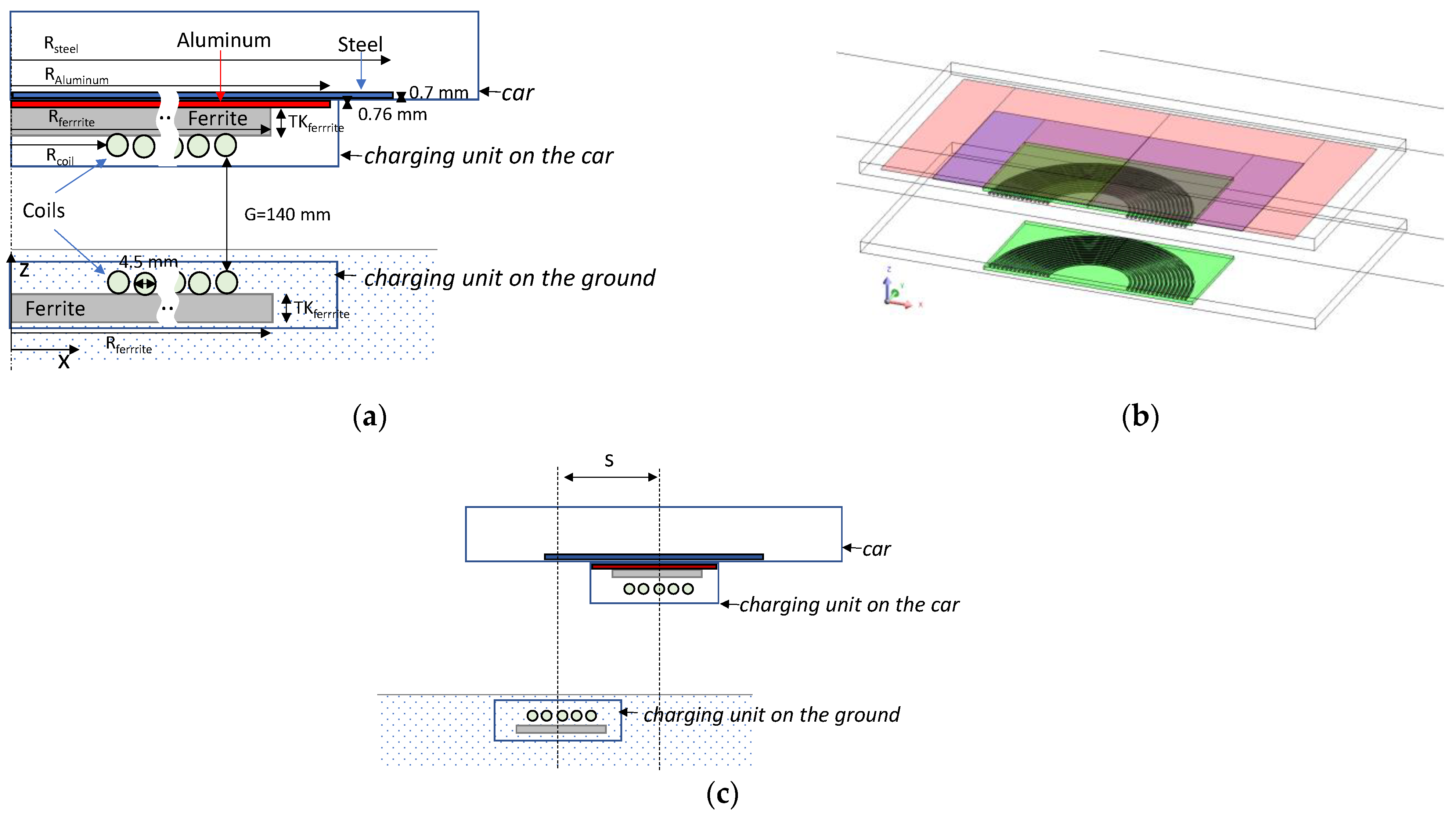
The field model is then coupled with a circuit model that includes the two coils, an ideal current source and a resistive load, i.e., the battery. The device geometry in Figure 1a shows the model of the car frame bottom (a steel sheet) equipped with the aluminum shield and the receiving coil magnetically coupled, the charging unit on the car, with the transmitting coil, the charging unit on the ground. Figure 1b shows the model implemented in Flux 3D (a commercial software released by Altair Engineering, Inc., Troy, MI, USA, https://altairhyperworks.com/product/flux, accessed on 1 March 2022). Both coils have 15-turns made of Litz wire and are endowed with ferrite concentrators. The load effect of the road, which at first glance is here assumed as a dielectric material, is not considered. All materials are considered linear and electrical characteristics are reported in

Table 1. Electrical characteristics of the material used in FEM model.

Material	Electrical Resistivity ρ [Ωm]	Relative Magnetic Permeability μr	Skin Depth [µm]
Ferrite	Non-conductive	3000	--
Steel	14 × 10−8	1000	20
Aluminum	2.6 × 10−8	1	240

. Figure 1c shows the cross-section of the recharging unit mounted on the car. In this figure, the shift of the charging unit on the car with respect to the charging unit on the ground is detailed. The shift parameter is labelled as s and it varies between 0, for the aligned case and 600 mm for the completely unaligned case.

The FE model solves a steady state AC magnetic problem through the scalar magnetic potential and vector electric potential formulation, coupled with the external electrical circuit. The device model is implemented using the Flux 3D code [16]. The magnetic time-harmonics field problem, based on the $\overline{\mathrm{T}}-\varphi$ formulation with $\overline{\mathrm{T}}$ electric vector potential and $\varphi$ the magnetic scalar potential, solves the following equation in the model domain:

$$\nabla \times \rho \nabla \times \overline{\mathrm{T}}+\mathrm{j}\mathsf{\omega }\mathsf{\mu }\left(\overline{\mathrm{T}}-\nabla \varphi \right)=0\text{.}$$

(1)

With ω angular frequency. The problem is subject to suitable boundary conditions. Then, the magnetic field $\overline{\mathrm{H}}$ is then given by:

$$\overline{\mathrm{H}}=\left(\overline{\mathrm{T}}-\nabla \varphi \right).$$

(2)

The $\overline{\mathrm{T}}-\varphi$ formulation is particularly useful because it allows to couple the field model with a circuit composed of linear electric components, like voltage or current sources, capacitors or inductors.

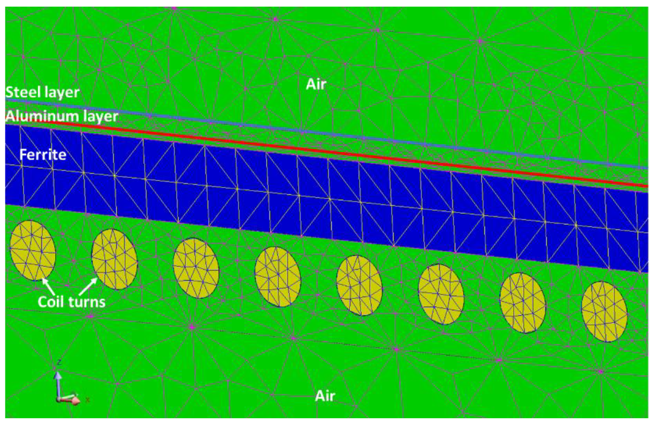
The coupled circuit allows us to easily modify the working conditions of the coils, like e.g., open circuit or forced current conditions, and computes relevant lumped parameters like self and mutual inductances. In this respect, from the field simulations the mutual and self-inductance values are evaluated. Figure 2 shows a particular of the mesh in a cross-section of the vertical plane. It is composed of 1,200,000 second-order tetrahedral elements. In particular, in the proposed model the mesh is composed of 76,756 surface elements for steel layer instead of 800 × 10⁶ surface elements (3.2 × 10⁹ volume elements). Moreover, the mesh of the aluminum layer contains only 40,000 surface elements instead of 450 × 10⁶ surface elements (1.35 × 10⁹ volume elements). Finally, in the proposed model, the mesh of the air volume around the device consists of 955,500 volume elements, only.

The mutual and self-inductances are calculated for different relative positions of the receiving and transmitting coil (step 50 mm) supplying A-B port with a current source at 85 kHz, as prescribed by SAE [8], and considering C-D port an open circuit and vice versa. Both the self-inductances of the receiving coil and the transmitting coil are evaluated separately, supplying the receiving and transmitting side at a time.

In particular, the self- and mutual inductances are evaluated at the pulsation ω (at f = 85 kHz) as follows:

• Mutual inductance, M: The voltage at the open circuit extremities at the receiving side, V_r, supplying the transmitting coil at I_t = 1A:

  $$M=\frac{V_r}{\omega I_t}$$

  (3)
• Self-inductance, L_t: The voltage at the transmitting coil supplying the transmitting coil at I_t = 1A.

  $$L_t=\frac{V_t}{\omega I_t}$$

  (4)
• Self-inductance, L_r: The voltage at the receiving coil supplying the receiving coil at I_r = 1A.

  $$L_r=\frac{V_r}{\omega I_r}$$

  (5)

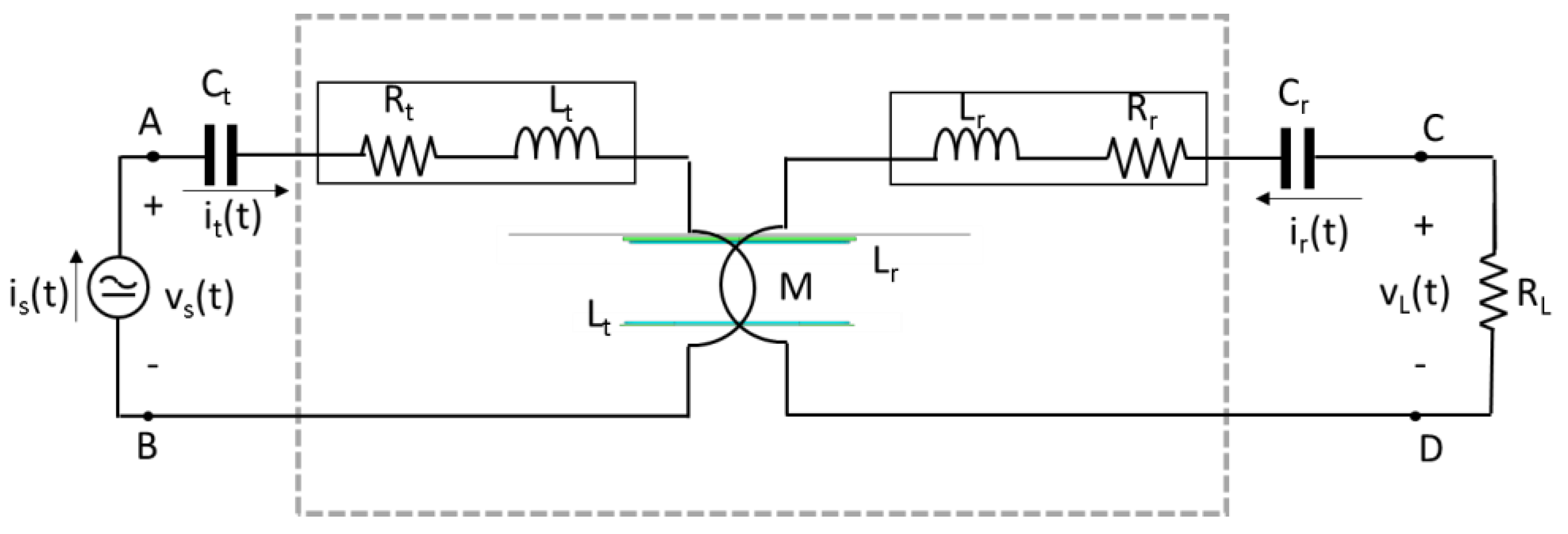
Figure 3 shows the coupling circuit in which two compensation capacitances are series connected to the coils. The series-connected capacitances are computed to obtain a resonance at the supply frequency.

The transmitting end of the FEM model is supplied using a current source and the receiving end is connected to the load, a resistance representing the battery.

3. Results and Discussion

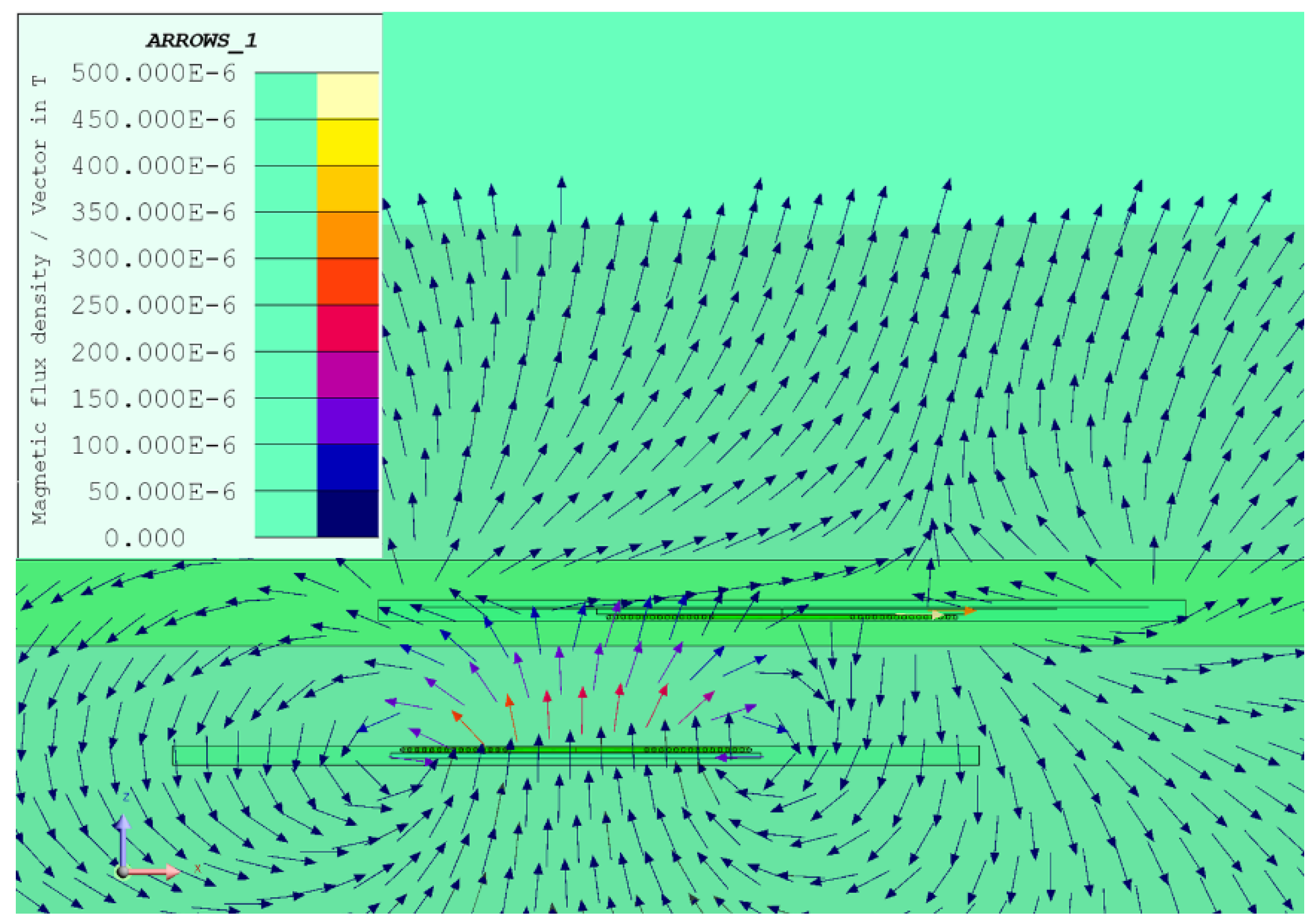
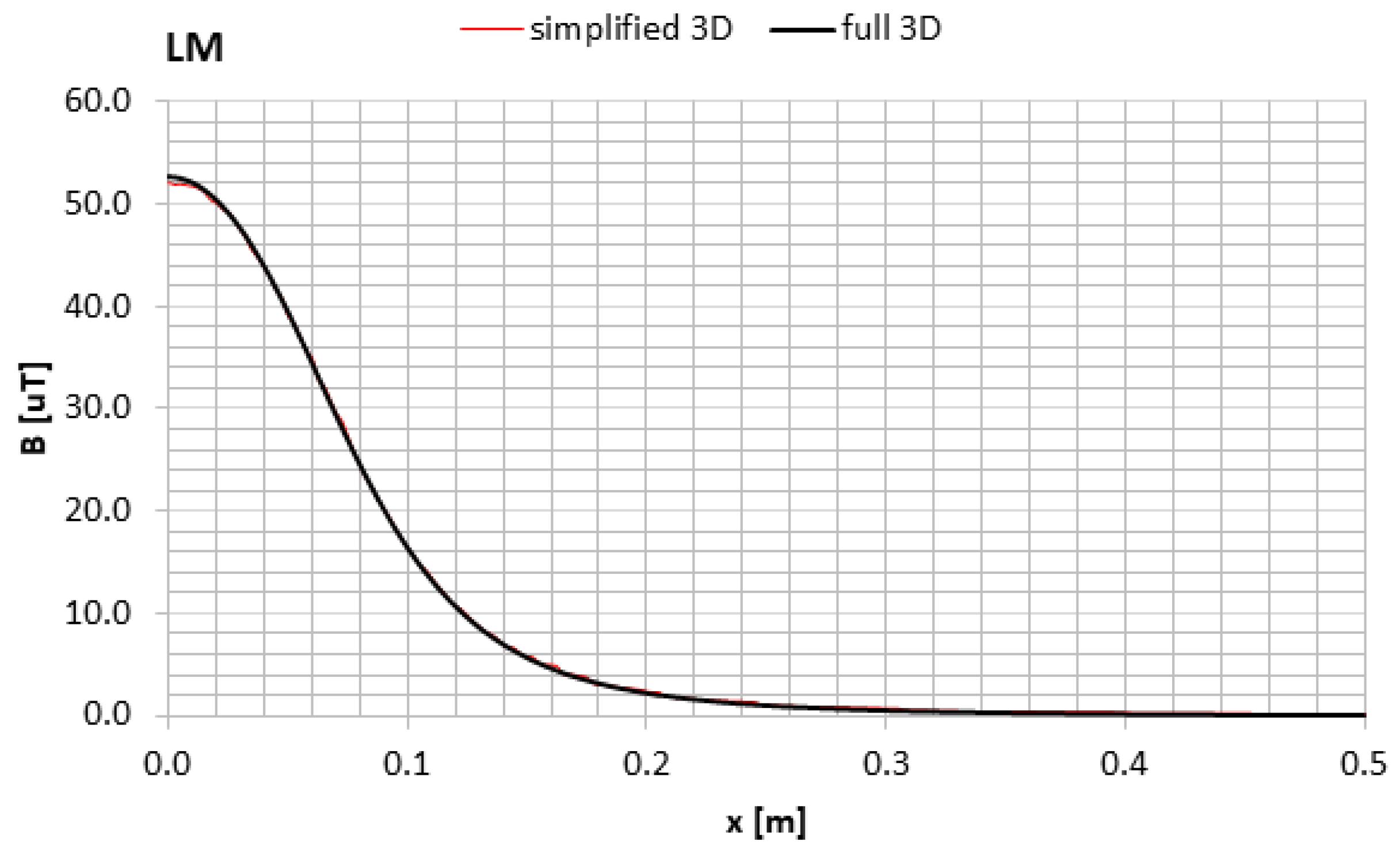
Figure 4 shows the magnetic flux density field; in particular the center line between the two coils (70 mm from both receiving and transmitting coils) along x-direction and for y = 0 (the same coordinate of coil centers) is considered.

The receiving coil is at no-load and the transmitting coil is supplied with a current of 1 A. For the sake of a comparison, the induction field calculated by means of the simplified 3D FE model with the shell elements and a full 3D FE model is represented in Figure 5.

The simplified 3D model is in accordance with the full 3D FE model; hence the simplified model is used for the subsequent calculations.

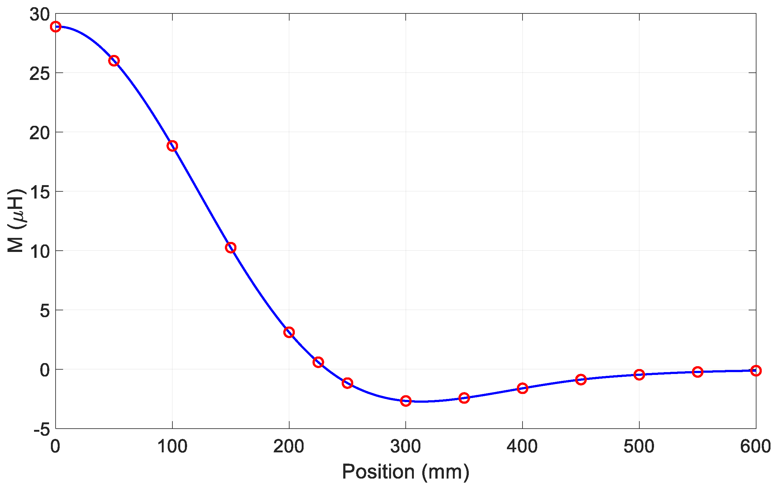
Accordingly, the mutual inductance calculated for different positions is shown in Figure 6 where the red circles denote the values of M obtained from (3) relevant to the positions considered in the FEM simulations. The solid blue line has been obtained by interpolation of the data coming from FEM.

As shown in Figure 6, there is a position of the receiving coil with respect to the transmitting coil in which the mutual inductance is zero even if the coils are still partially faced. Some authors denote this condition as the “zero power point” because, when it happens, no power can be transmitted between the two coils. The magnetic flux density map of the cross-section of the device at the M = 0 point is shown in Figure 4.

In order to analyze the zero-inductance effect, future work will study the mutual inductance of the two coils by also considering the effect of neighboring transmitting coils.

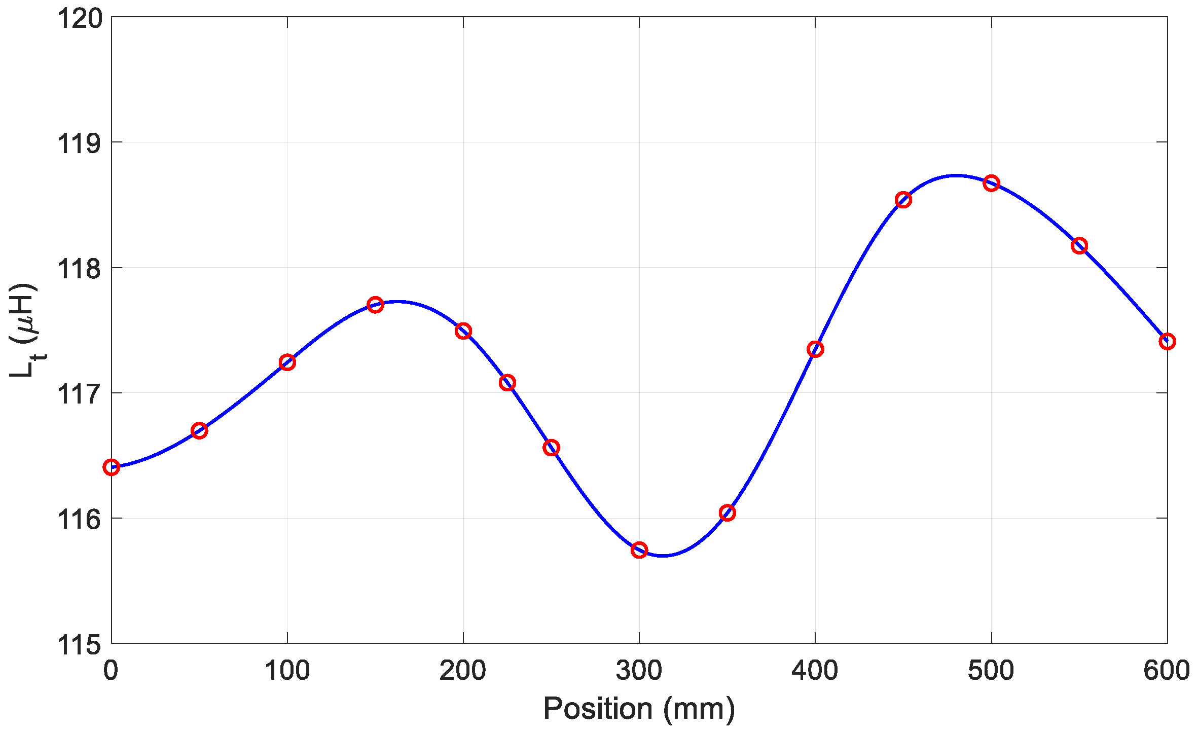
The self-inductances of the coupling coils, obtained from (4) and (5), are not very sensitive to the relative coil position. As shown in Figure 7, the self-inductance of the transmitting coil changes of about 2.5% along the full span of the considered positions.

Table 2. Self and mutual-inductance for different positions.

Dx [mm]	0	50	100	150	200	225	250	300	350	400	450	500	550	600
M [μH]	28.9	26.0	18.8	10.3	3.1	0.6	−1.2	−2.7	−2.4	−1.6	−0.9	−0.5	−0.2	−0.1
Lt [μH]	116.4	116.7	117.2	117.7	117.5	117.1	116.6	115.7	116.0	117.3	118.5	118.7	118.2	117.4
Lr [μH]	113.2	113.2	113.2	113.0	112.7	112.5	112.0	111.1	110.5	110.1	110.1	110.0	110.1	110.1

reports the self and mutual inductances evaluated using Equations (3)–(5) for different positions of the receiving coil with respect to the transmitting coil. The values relevant to the aligned coil position, listed in the first column of the table, are in good agreement with those obtained experimentally from the prototype described in [7], which resulted 31 μH, 120 μH and 118 μH, respectively.

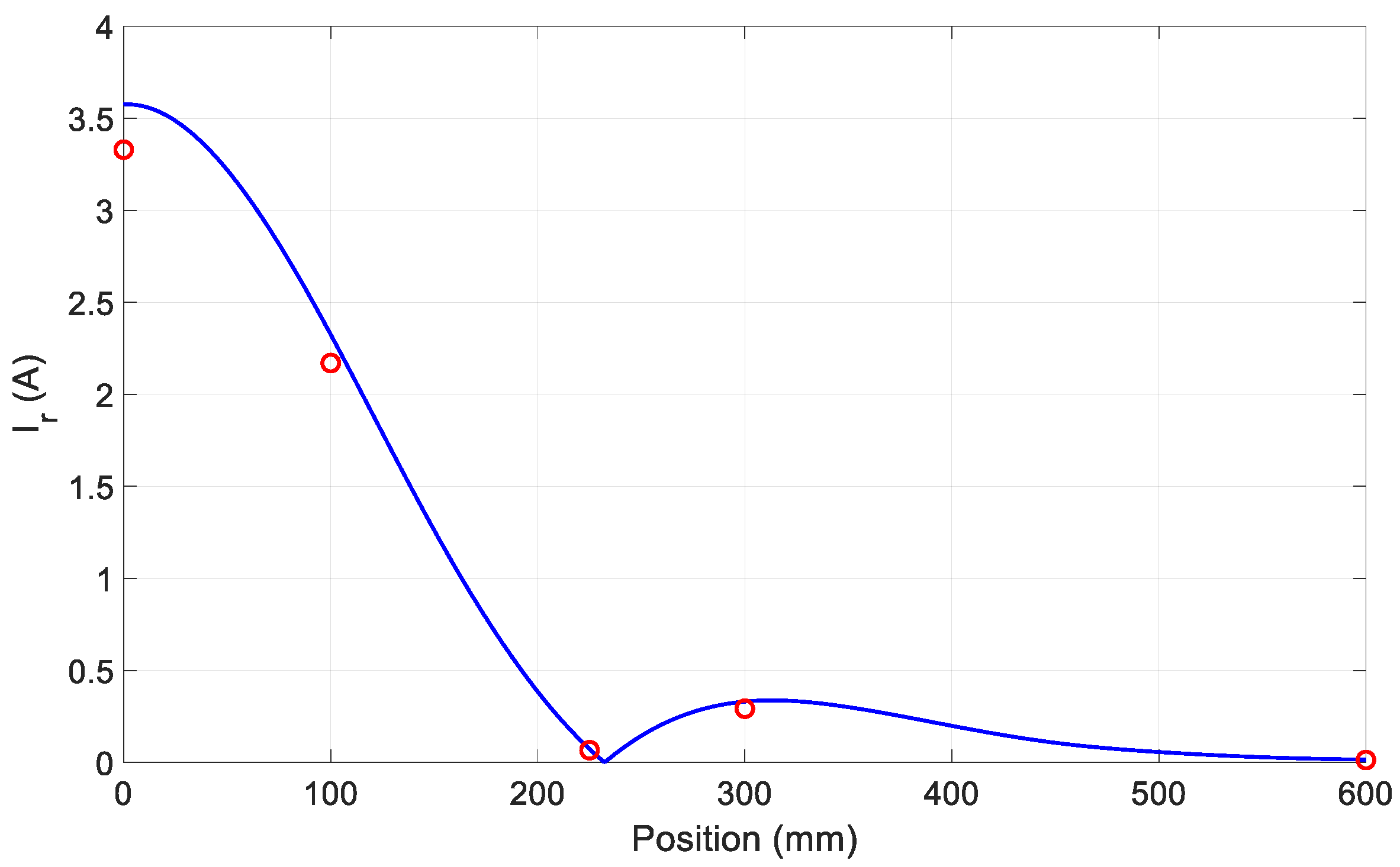
For the sake of a comparison, the amplitude of the current I_r in the receiving coil is calculated with the transmitting coil supplied with 1 A_rms in a twofold way: first using the circuit-field model in Figure 3 and next solving an independent circuit with the self and mutual-inductance identified according to (3)–(5). Figure 8 shows the amplitudes of I_r coming from FEM with the red circles while the blue line represents the values computed with the independent circuit.

The agreement between the FEM simulations and the analytical results is good in all the considered positions, especially when the coils are misaligned. The figure confirms that at the zero power point the receiving coil is not supplied with any power because the current amplitude is null.

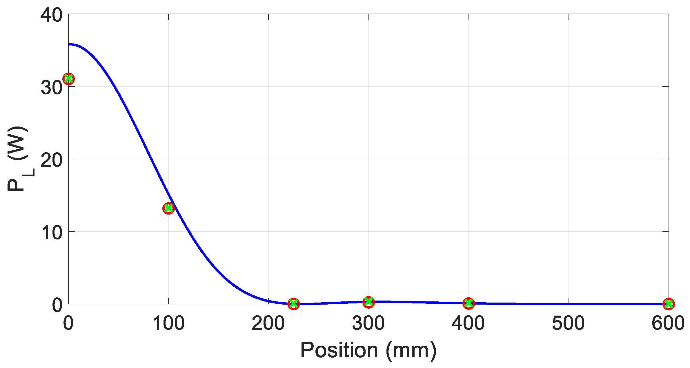
This condition is also confirmed in Figure 9, which compares the power P_L transferred to the load obtained from the FEM simulation and the computation with the independent circuit. First, the power obtained by FEM is calculated on the load whereas the one coming from the computation with independent circuit also encompasses the losses in the aluminum and steel shields. Being that the losses are very small, they do not sensibly affect the results. In fact, after re-calculating the total power losses (the sum of the power transferred to the load and the losses in the shields, green stars in Figure 9), they are almost coincident to the red circles. In this case, the results from FEM and circuit analysis are also in good agreement, especially when the coils are not perfectly aligned.

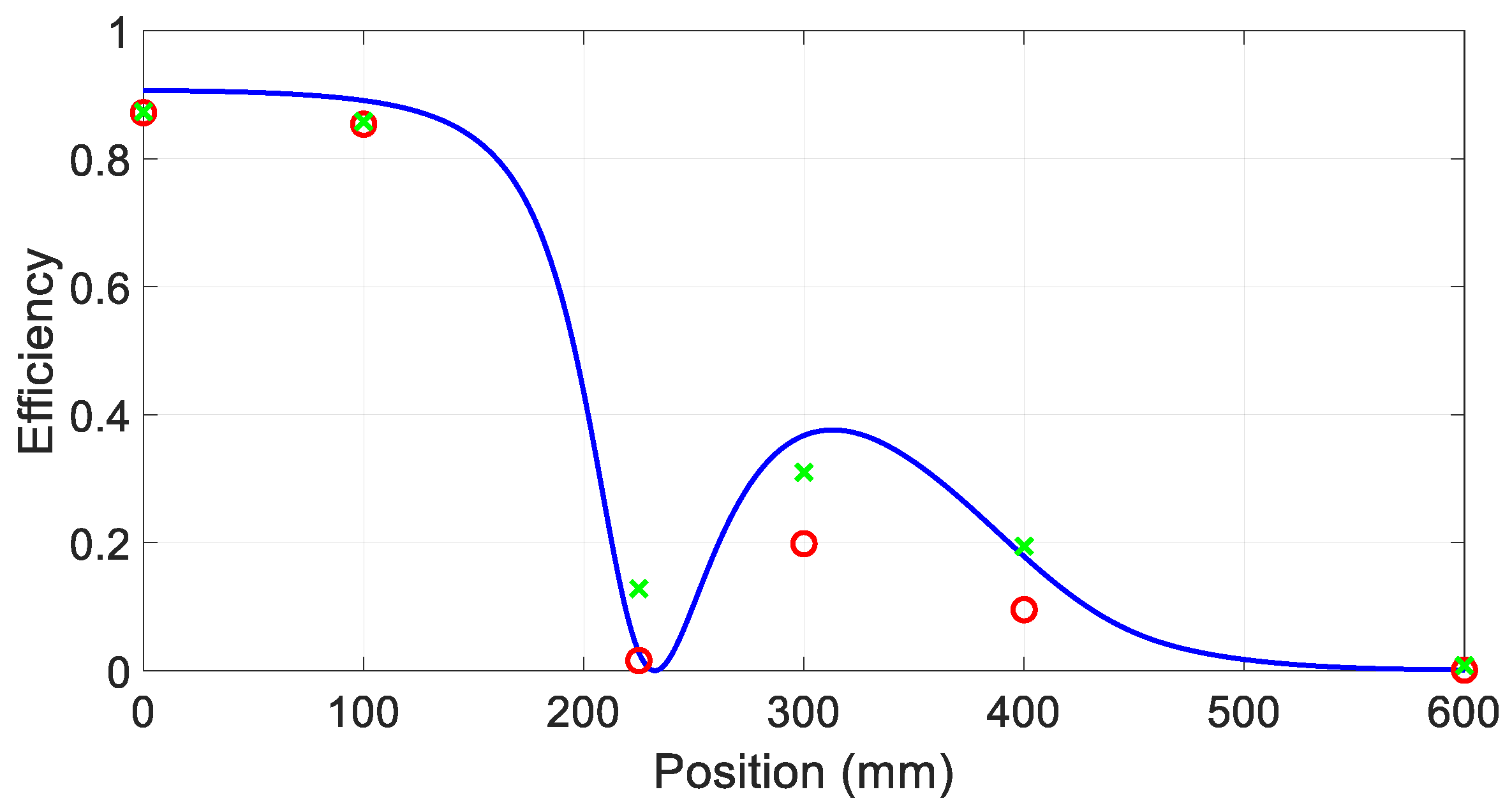
Behaviors similar to those reported in Figure 9 have also been obtained for the power P_S supplied by the current generator connected to the transmitting coil. The ratio P_L/P_S gives the power transfer efficiency of the WPTS. It is reported in Figure 10. In this case the real value of the efficiency is given by the red circles, obtained from FEM considering only the power P_L delivered to the load. The green stars are obtained by adding to P_L the power lost in the shields and have been plotted to make a comparison with the blue line coming from the computation with the independent circuit. As explained about Figure 9, the latter considers together the losses and the load power so that the computed efficiency results higher than the real one. Despite the small values of the losses, they have a sensible effect on the system efficiency when the transferred power is small, and this explains why the difference between the red circles and the green stars initially increases with the misalignment. When the misalignment is very high both the load power and the losses are small while the losses in the transmitting coil remain constant thus forcing both the stars and the circles to move toward zero.

4. Conclusions

The paper presents an approach to study the coupling characteristics of dynamic WPTSs by FE models with reduced computational load. To this end, the shell formulation is applied to the steel and thin aluminum sheets deployed on the receiving coil thus obtaining a simplified 3D model of the system. After validating the simplified model by comparing its outcomes with those of a full 3D model, it is used in a number of FEM simulations to work out the coils mutual and self-inductances in different positions. Considering the same positions, the simplified model is also used to assess the current flowing in the WPTS load once the supply current and the relative position of the coils have been set. These data are used to validate an equivalent circuital model based on the inductive elements identified by the FEM simulations and that allows to analyze the functioning of the WPTS without using FEM simulations.