A NARX Model to Predict Cabin Air Temperature to Ameliorate HVAC Functionality

Abstract

Vehicular technology has integrated many features in the system, which enhances the safety and comfort of the user. Among these features, heating, ventilation, and air conditioning (HVAC) is the only feature that maintains the set cabin air temperature (CAT). The user’s command drives the set CAT, and the thermostat provides feedback to the HVAC to maintain the set CAT. The CAT is increased by extracting the heat from the engine surface produced by the fuel combustion, whereas the CAT is reduced by the known processes of the air conditioning system (ACS). Therefore, the CAT driven by the user’s command may not be optimal, and estimating the optimal CAT is still unsolved. In this work, we propose a new process where the user can input a range for CAT instead of a single value. Optimal HVAC criteria were defined, and the CAT was estimated by performing iterative analysis in the user-selected range satisfying the criteria. The HVAC criteria were defined based on two measurable parameters: air conditioning refrigerant fluid pressure (ACRFP) and engine surface temperature (EST) empirically defined as the vector CATOP. In this article, a NARX DL model was used by mapping the vehicle-level vectors (VLV) to predict the CATOP in real-time using field data obtained from a 2020 Cadillac CT5 test vehicle. Utilising the DL model, CATOP for future time steps was predicted by varying the CAT in the definite range and applying HVAC criteria. Thus, an optimal set CAT was estimated, corresponding to the optimal CATOP defined by the HVAC criteria. We performed the validation of the DL model for multiple datasets using traditional statistical techniques, namely, signal-to-noise ratio (SNR) values, first-order derivatives (FOD), and root-mean-square error (RMSE).

1. Introduction

The automotive industry’s evolution has influenced every engineering aspect, including materials science, thermal engineering, and control theory [1]. In an internal combustion engine-driven vehicle, the thermal energy produced by the combustion process is exchanged between the ambiance, engine components, HVAC, lubrication oil, and coolant [2]. HVAC is the only module integrated into the vehicle functions to maintain the CAT set by the user, and in this article, we propose a novel methodology to predict the set CAT. It is known from the existing literature that the CAT is reduced by the ACS [3] and increased by extracting heat from the engine surface, as shown in Figure 1 [4,5].

Ref. [6] adopted an adaptive control technique to alter the functioning of the ACS based on environmental conditions and driver behaviour. This method produced simulation results that project 1% more energy-saving than the conventional fuzzy logic control used by [7]. The fuzzy logic control developed in [7] contained an iterative analysis of CAT and the ACS compressor load to evaluate the system’s performance, including reduced energy consumption [7]. Ref. [8] developed an ACS to produce a desirable CAT and maintain the air quality in conjunction with the engine controller by activating cruise control. Refs. [9,10] investigated the parameters of the mass flow rate of the air by dynamically adjusting the blower speed and air-gates opening under various thermal loads, which resulted in reduced energy consumption. Ref. [11] developed a heat balance method for estimating the thermal load encountered by the cabin using a predictive model mapping the driving conditions. This method could potentially predict thermal comfort in real-time and thus reduce the power consumption of the ACS. Finally, Ref. [12] developed an optimised control model for three stages to enhance the efficiency of the ACS. These stages include optimising the ACS operating point based on the control inputs and relevant actuators.

All the models developed to optimise the HVAC system have automated functionality developed by engineers and do not involve the user’s input. The user’s input in real-time is defined as DBV consisting of the elements (Speeding, Steering, CAT). Ref. [13] proposed a novel methodology to predict Speed, and in this article, we propose to predict CAT utilising similar concepts. Also, none of the existing literature proposed a model that can generate a unique CAT driven by the user’s command to augment the HVAC efficiency. In this article, we propose a method to predict the CAT profile in a definite range defined by the user (e.g., [65 70] °F or [70 75] °F), analogous to [13].

Inspired by the research [13,14], a similar NARX DL model was developed, mapping the elements VLV— [Odometer, DBV, EAT] and CATOP—EST and ACRFP (HVAC). CATOP is an empirical parameter defined to represent the HVAC elements, and optimal HVAC criteria are defined and applied to the predicted CATOP in real-time. We estimated a unique CAT value by the interactive analysis, and the detailed procedure adopted is shown in the following sections. The rest of the article is organised as follows: Section 2 and Section 4 propose predicting CATOP and CAT, whereas Section 3 defines the optimal HVAC criteria applied to the CATOP to generate an optimal CAT profile. In Section 5, the detailed results of the predictive model and experimental techniques are presented.

2. Predictive Model—CATOP

We discuss the NARX DL model elements to predict CATOP—ACRFP and EST in this section.

2.1. Modelling

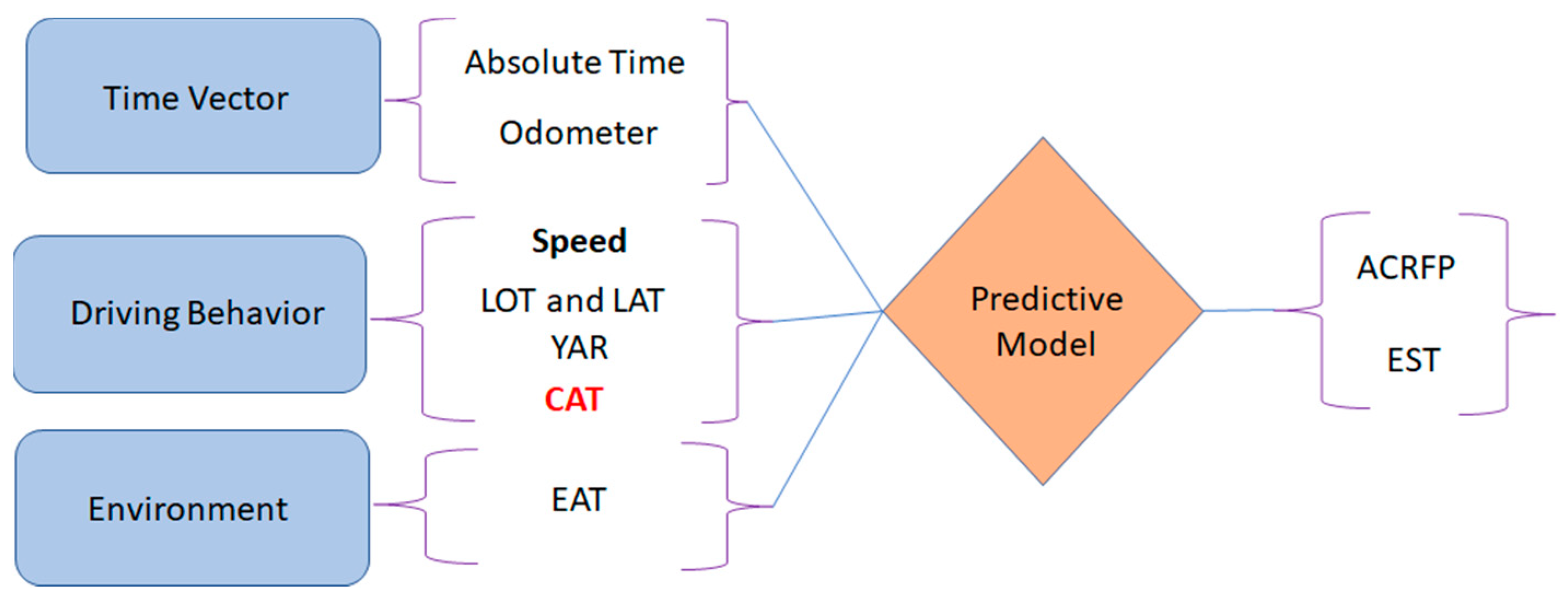
The NARX DL model is developed mapping the VLV—(Time step, Odometer, DBV, EAT) and CATOP— (EST, ACRFP) (Figure 2) with default training properties [14]. The DBV is defined with five parameters (Speed, LOT, LAT, YAR, CAT), which are the user’s prerogative in real-time [15]. The parameters EAT and CAT influence thermal stress on the engine [16], whereas the odometer reading reflects the age of the vehicle. This article does not consider the remaining VLV elements (vehicle posture [17], aerodynamics, tire pressure) as their effects are assumed to be insignificant. Also, the orientation of the RRC vector is insignificant for the analysis; thus, positive values of LAT and YAR are considered in developing the DL models. The purpose of selecting EST and ACRFP as outputs and methodology to develop the DL models are discussed in Section 3 [18] and Section 5.2.

3. Optimal CATOP Criteria

In the existing literature, researchers optimised the HVAC system by applying the constraint of fuel economy [19]. However, the experimental results reflect the fuel saved per trip being <2%, and none of the techniques had involved the parameter CAT (°F). Deviating from the traditional concept of optimising fuel economy, based on the real-time data retrieved (Section 5.1), two parameters, EST (°F) and ACRFP (PSI), that reflect HVAC performance were identified. EST (°F) is maintained in a specific range to achieve optimal thermal stress on the engine by transferring heat to four main elements—engine oil, cabin, coolant/radiator, and external ambience [20].

Similarly, the ACS functionality is affected by multiple parameters, including compressor load, engine fan speed, and power consumed. However, by analysing the real-time test data (Section 5.1), we conclude that variations of these parameters were insignificant due to changes in CAT (°F). Hence, we considered ACRFP (PSI) as the CATOP element, which showed substantial fluctuations by varying EAT (°F) and CAT (°F).

3.1. CATOP Element—EST

It is known from the existing literature that optimal thermal stress on the engine components and ideal engine oil viscosity is achieved when EST = 90 °C (194 °F) [21]. Hence, the conformance between the predicted EST ($ES{T}_p$) and ideal EST ($ES{T}_i$ = 90 °C) must be minimal for optimal HVAC functionality. The real-time test data depict that EST (°F) recorded was observed in the range of [165 220] °F.

Hence, we define two empirical parameters [A1 A2] to split the scenarios representing the cases when the predicted EST ($ES{T}_p$) > 90 °C and < 90 °C. The parameters [A1 A2] are plotted for the snippet of the test case (1 km), and the area under the curve is evaluated [Area_A1, Area_A2]. Hence, the minimum value of the parameters [Area_A1, Area_A2] is considered the criteria for the element EST (°F).

$$A1=\left(ES{T}_p-ES{T}_i\right), if ES{T}_p>ES{T}_i=90 °\mathrm{C}.$$

$$A1=0, if ES{T}_p<ES{T}_i=90°\mathrm{C}=194°\mathrm{F}.$$

$$A2=\left(ES{T}_i-ES{T}_p\right), if ES{T}_p \le ES{T}_i=90 °\mathrm{C}.$$

$$A2=0, if ES{T}_p \ge ES{T}_i=90 °\mathrm{C}=194 °\mathrm{F}.$$

3.2. CATOP Element—ACRFP

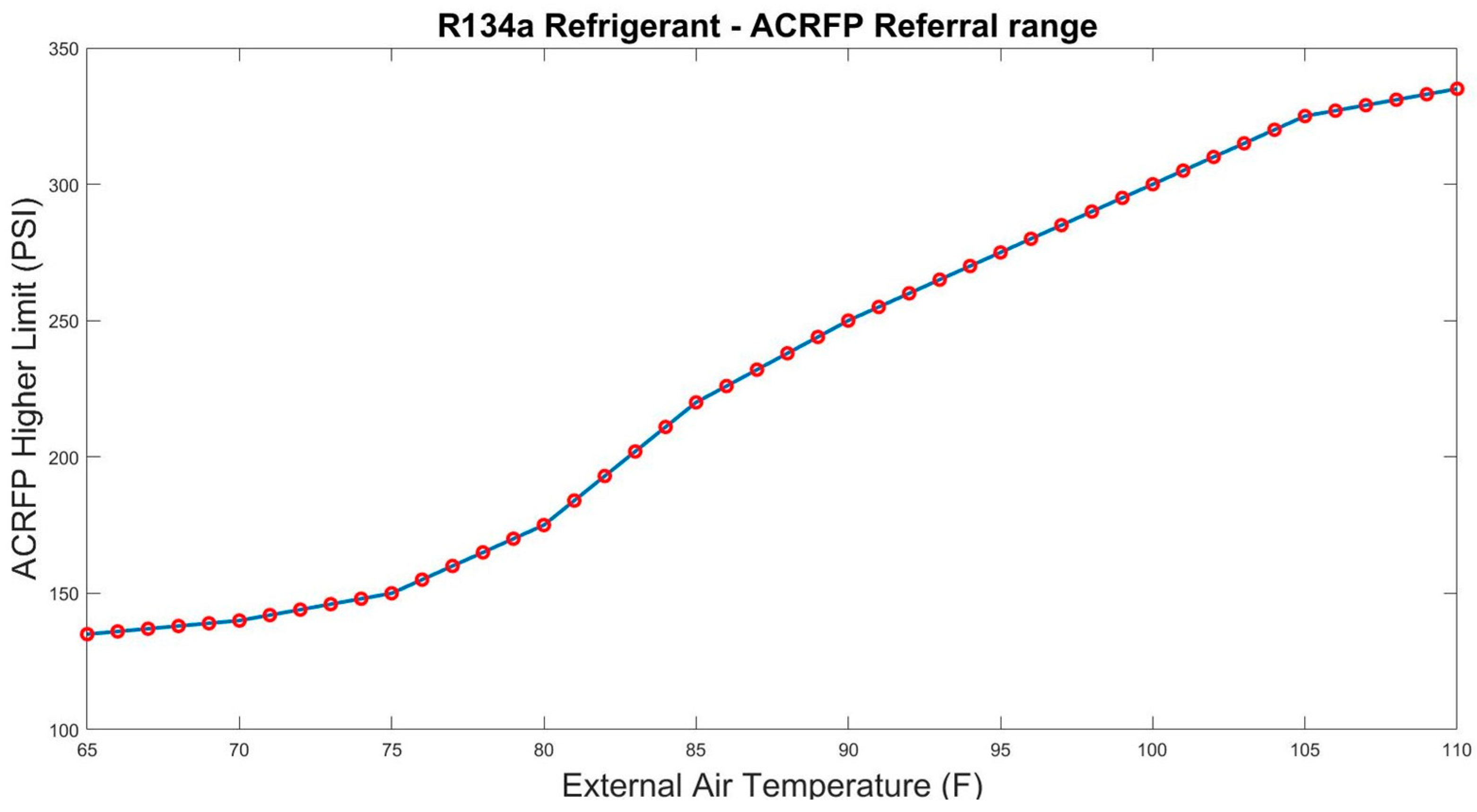
The ACS of the test vehicle was assumed to function with the refrigerant R134a. The ideal functioning of the ACS was defined by correlating the upper boundary limits of the ACRFP for the corresponding EAT (°F) [22]. We show these values in Figure 3 and Table S2, and the intermittent higher boundary values of ACRFP (PSI) for EAT (°F) in the range [65 110] °F could be estimated by basic linear interpolation. Hence, an empirical parameter B (PSI) is defined, representing the conformance of the predicted $ACRF{P}_p$ and threshold $ACRF{P}_h$. The threshold $ACRF{P}_h$ is estimated by correlating the recorded EAT using the plot shown in Figure 3. In a generic case, this value is significant when EAT < 65 °F.

$$B=\left(ACRF{P}_p-ACRF{P}_h\right),ifACRF{P}_p>ACRF{P}_h$$

$$B=0,if ACRF{P}_p \le ACRF{P}_h \mathrm{or}\mathrm{EAT}<65°\mathrm{F}$$

Similar to the previous criteria, parameter B is plotted for the test case snippet, and Area_B represents the area under curve B. Therefore, minimum Area_B was considered the optimal HVAC criteria corresponding to the element ACRFP (PSI).

3.3. Smoothness Measure—EST and ACRFP

In this research, we developed the CATOP conformance vector Area = [Area_A1, Area_A2, Area_B] plots for the test case snippets 100 steps (1 step = 10 m). Along with the area under the curve, we considered the smoothness measure (S) for the plots [A1 A2 B] as the third optimal HVAC criterion. The spline fit was embedded into the curves [A1 A2 B] using the built-in functions of MATLAB [13].

$$\mathrm{S}=[R^2,\mathrm{Adj}{R}^2,\mathrm{SSE},\mathrm{RMSE}]$$

The vector S represents the smoothness measure vector estimated using the traditional statistical techniques $R^2$/Adj $R^2$ and SSE/RMSE. $R^2$ is a statistical measure of how close the data are to the fitted regression line, whereas Adj $R^2$ is a modified version of $R^2$ adjusted for the number of predictors in the model, which is always lower than $R^2$. SSE is the residual sum of squares of the conformance between the predicted and fitted curve, and the square root of the mean SSE represents RMSE. Higher values of $R^2$/Adj $R^2$ and lower SSE/RMSE were considered a good fit for the curve [13]. $R^2$/Adj $R^2$ values range between [0 1], representing the percentage of match, whereas SSE/RMSE have the same units of the parameters. Therefore, the vector S is estimated individually for the plots [S_A1 S_A2 S_B] by fitting a spline using the built-in toolboxes of MATLAB. The mathematical models of vector S are not the scope of this article.

4. Prediction of CAT

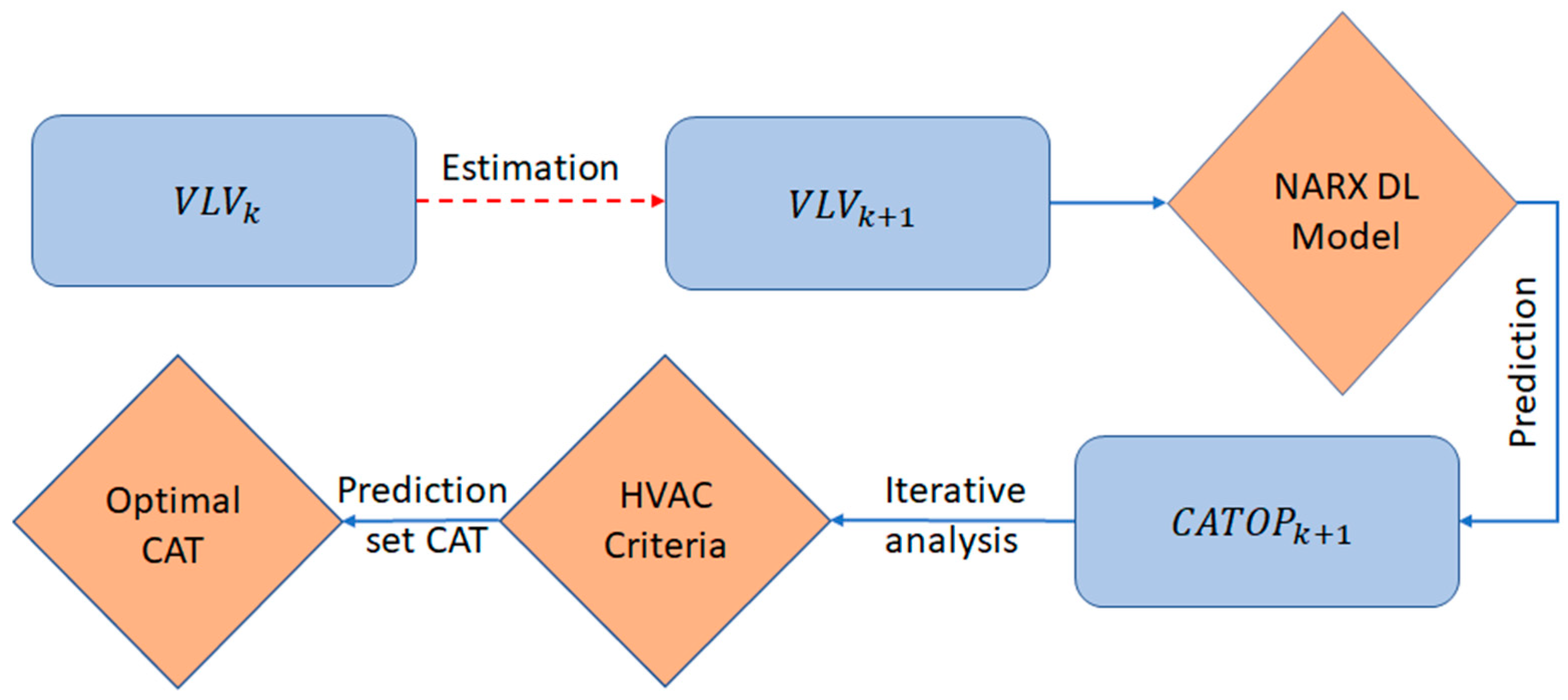
In this research, we challenged the constant CAT (°F) set by the user, and a novel model to predict optimal CAT profile in a definite user-defined range was developed. The default range of allowable CAT, [65 70] °F for EAT > 65 °F and [70 75] °F for EAT < 65 °F, are considered. In the following sections, we estimate the optimal CAT for future steps by following the process shown in Figure 4 [13].

4.1. Estimation of Future Inputs—NARX DL Model

Step 1: We estimated the future input states ($VL{V}_{k+1}$) of the DL model relative to the vehicle’s current state ($VL{V}_k$) by the equation set shown in

Table 1. Equation Set—Prediction of future input states.

$T_{k+1}=T_k+ dT$(s)	$O_{k+1}=O_k+S_k.dT$ (km)	$EA{T}_{k+1}=EA{T}_k$ (°F)		$S_{k+1}=S_k$ (MPH)
$L_{o\left(k+1\right)}=$ $g{\mu }_r$+ $gsin({\theta }_{\left(k+1\right)g)})$ + $\frac{\rho C_d.A_c}{2.\left(M_c+M_L\right)}$ $·S_{k+1}^2$ (m·${\mathrm{s}}^{-2}$)
$2RR{C}_{k+1}=\frac{S_{k+1}^2}{L_{a\left(k+1\right)} }+\frac{S_{k+1}}{Y_{a\left(k+1\right)}}$, $min \left[abs\left(Y_{a\left(k+1\right)}·S_{k+1}-L_{a\left(k+1\right)}\right)\right]$
g = 9.81 m·${\mathrm{s}}^{-2}$	${\mu }_r$= 0.013	$\rho$ = 1.225 kg·${\mathrm{m}}^{-3}$	$C_d$ = 0.31	$A_c$ = 1.71 ${\mathrm{m}}^2$
$CA{T}_{k+1}=\left[65 70\left] \left(°\mathrm{F}\right) \mathrm{or} \right[70 75\right] \left(°\mathrm{F}\right)$		2020 Cadillac CT5: $M_c$ = 1769.69 kg, $M_L$ = 78.7 kg (Load)

. The magnitude of the odometer reading $O_{k+1}$(km) and timestep $T_{k+1}$(s) is estimated using basic interpolation, and the vehicle’s speed $S_{k+1}$ = SL (MPH) since ACCSSP ≈ SL.

The parameters YAR ($Y_{a\left(k+1\right)}$) and LAT ($L_{a\left(k+1\right)}$) are estimated using the equations, framed assuming ISB [23], whereas as LOT ($L_{o\left(k+1\right)}$) is calculated based on the vehicle resistance as shown in Table 1. The vehicle is assumed to be integrated with infotainment and connectivity features, which assist our work to retrieve the terrain parameters [$RR{C}_{k+1}$, ${\theta }_{g\left(k+1\right)}$], along with $EA{T}_{k+1}$ based on the GPS location and infotainment maps (e.g., Super and Ultra cruise features integrated into the Cadillac vehicle segment—GMC) [13].

We varied $CA{T}_{k+1}$(°F) in a specific default range based on $EA{T}_{k+1}$(°F). A sample set of the future input states ($VL{V}_{k+1}$) of the DL model for 100 steps are presented in

Table 2. Estimation of Future Inputs—DL Model, 2020 Cadillac CT5 (100 steps = 1000 m) [13].

Step	Odometer (km)	Speed (MPH)	RRC (m)	YAR $(\mathbf{rad}·{\mathbf{s}}^{-1})$	LAT $(\mathbf{m}·{\mathbf{s}}^{-2})$	LOT $(\mathbf{m}·{\mathbf{s}}^{-2})$	EAT (°F)	CAT (°F)
$D_0$	15,000	70	8304.140	0.216	0.1179	0.4375	78.5, 38.3	[65 70], [70 75]
$d{D}_{10}$	15,000.1	70	8304.140	0.216	0.1179	0.375	78.5, 38.3	[65 70], [70 75]
$d{D}_{20}$	15,000.2	70	8304.140	0.216	0.1179	0.3125	78.5, 38.3	[65 70], [70 75]
$d{D}_{30}$	15,000.3	70	9342.157	0.192	0.1048	−0.125	78.5, 38.3	[65 70], [70 75]
$d{D}_{40}$	15,000.4	70	24,912.42	0.072	0.0393	−0.1875	78.5, 38.3	[65 70], [70 75]
$d{D}_{50}$	15,000.5	70	74,737.261	0.024	0.0131	−0.0625	78.5, 38.3	[65 70], [70 75]
$d{D}_{60}$	15,000.6	70	74,737.261	0.024	0.0131	0.25	78.5, 38.3	[65 70], [70 75]
$d{D}_{70}$	15,000.7	70	37,368.630	0.048	0.0262	0.25	78.5, 38.3	[65 70], [70 75]
$d{D}_{80}$	15,000.8	70	24,912.420	0.072	0.0393	0.1875	78.5, 38.3	[65 70], [70 75]
$d{D}_{90}$	15,000.9	70	24,912.420	0.072	0.0393	0.1875	78.5, 38.3	[65 70], [70 75]
$D_{100}$	15,001	70	9342.157	0.192	0.1048	0.3125	78.5, 38.3	[65 70], [70 75]

.

4.2. Prediction of Outputs—NARX DL Model

Step 2: Six input sets (1 set = 1000 m) are developed by varying the CAT in the user-defined range [65 70] °F, based on step 1. We fed the input sets into the NARX DL model and predicted the corresponding output sets (CATOP vectors). We adopted a similar procedure for the winter case scenario with CAT = [70 75] °F. The properties and precision of the prediction of the DL model are discussed in Section 5.2.

4.3. Implementation—HVAC Criteria

Step 3: We determined the corresponding CATOP conformance vector [A1 A2 B] by analysing the predicted output sets. The optimal HVAC criteria were applied, and we estimated the performance vector [Area, $R^2$, Adj $R^2$, SSE, RMSE] for every set of outputs (

Table 3. Iterative Analysis—DL Model, 2020 Cadillac CT5 (10 steps = 100 m) [13].

CAT	A1					A2					B
°F	Area	R	$\mathbf{Adj}{\mathit{R}}^{\mathbf{2}}$	SSE	RMSE	Area	R	$\mathbf{Adj}{\mathit{R}}^{\mathbf{2}}$	SSE	RMSE	Area	R	$\mathbf{Adj}{\mathit{R}}^{\mathbf{2}}$	SSE	RMSE
ACCSSP = 70 MPH; EAT = 78.75 °F
65	114.5	0.994	0.986	1.495	0.194	1931	0.998	0.994	61.03	1.242	2252	0.995	0.989	158.9	2.004
66	175.2	0.995	0.987	2.749	0.264	1994	0.998	0.994	64.36	1.275	2365	0.996	0.989	167.8	2.059
67	216.5	0.992	0.979	6.555	0.407	2020	0.998	0.994	67.47	1.306	2379	0.996	0.990	149.4	1.943
68	203.8	0.992	0.981	5.391	0.369	1872	0.997	0.993	67.63	1.307	2399	0.996	0.990	155.5	1.983
69	178.2	0.993	0.982	3.933	0.315	1688	0.997	0.993	52.16	1.148	2402	0.996	0.990	167.6	2.058
70	201.9	0.995	0.986	3.773	0.309	1612	0.998	0.994	44.56	1.061	2416	0.996	0.990	162.6	2.027
ACCSSP = 70 MPH; EAT = 38.3 °F
70	47.069	0.990	0.976	0.551	0.118	40.095	0.987	0.968	0.938	0.154	0.000	0.000	0.000	0.000	0.000
71	45.876	0.990	0.975	0.557	0.119	40.662	0.987	0.968	0.961	0.156	0.000	0.000	0.000	0.000	0.000
72	45.408	0.990	0.975	0.561	0.119	41.013	0.987	0.968	0.978	0.157	0.000	0.000	0.000	0.000	0.000
73	45.575	0.990	0.975	0.566	0.120	41.169	0.987	0.968	0.988	0.158	0.000	0.000	0.000	0.000	0.000
74	46.270	0.990	0.975	0.569	0.120	41.162	0.987	0.968	0.993	0.158	0.000	0.000	0.000	0.000	0.000
75	47.368	0.990	0.975	0.572	0.120	41.026	0.987	0.967	0.993	0.158	0.000	0.000	0.000	0.000	0.000

). Based on these values, we identified the top three CAT values, satisfying the CATOP criteria for 100 m shown in

Table 4. Eligible CAT Values: Iterative Analysis—Optimal CATOP. (10 steps = 100 m).

A1					A2					B
Area	R	$\mathbf{Adj}{\mathit{R}}^{\mathbf{2}}$	SSE	RMSE	Area	R	$\mathbf{Adj}{\mathit{R}}^{\mathbf{2}}$	SSE	RMSE	Area	R	$\mathbf{Adj}{\mathit{R}}^{\mathbf{2}}$	SSE	RMSE
ACCSSP = 70 MPH; EAT = 78.75 °F
65	66	66	65	65	70	66	66	70	70	70	67	67	67	67
66	70	70	66	66	69	65	65	69	69	69	68	68	68	68
69	65	65	70	70	68	67	67	65	65	68	70	70	65	65
ACCSSP = 70 MPH; EAT = 38.3 °F
72	70	70	70	70	70	71	71	70	70	70	70	70	70	70
73	71	71	71	71	71	70	70	71	71	71	71	71	71	71
71	72	72	72	72	72	72	72	72	72	72	72	72	72	72

. Therefore, we framed the CAT matrix for 1000 m for two scenarios, as shown in

Table 5. ACCSSP = 70 MPH: Optimal CAT Matrix—(100 steps = 1 km).

CAT Matrix
EAT = 78.75 (°F)										EAT = 38.3 (°F)
$d{T}_1$	$d{T}_2$	$d{T}_3$	$\mathrm{d}{T}_4$	$\mathrm{d}{T}_5$	$d{T}_6$	$d{T}_7$	$d{T}_8$	$d{T}_9$	$d{T}_{10}$	$d{T}_1$	$d{T}_2$	$d{T}_3$	$\mathrm{d}{T}_4$	$\mathrm{d}{T}_5$	$d{T}_6$	$d{T}_7$	$d{T}_8$	$d{T}_9$	$d{T}_{10}$
66	66	66	68	68	65	66	66	68	66	70	70	70	70	70	70	72	70	71	73
67	67	67	66	69	66	67	67	66	67	71	71	71	71	71	71	70	71	72	74
65	65	65	67	70	67	65	65	67	65	72	72	72	72	72	72	71	72	70	75

.

4.4. Estimation of Optimal CAT

Step 4: The CAT matrix (3 × 10) results in a maximum of $3^{10}$ possible CAT profiles for 1000 m. In the final step, we proposed the following algorithm to identify the unique CAT profile [13].

Algorithm to Estimate CAT

• Assuming the set CAT at step k was $C_k$, if the eligible CAT’s were either $C_k$+1, $C_k$, or $C_k$−1, then the highest magnitude among the three was selected as $C_{k+1}$, for the case $EA{T}_k \ge 65 °\mathrm{F}$ and selected the lower value as $C_{k+1}$ for the case $EA{T}_k<65 °\mathrm{F}$.
• We chose the value of $C_{k+1}$ closer to $C_k$. If this resulted in two values, the higher value was considered $C_{k+1}$ for the case $EA{T}_k \ge 65 °\mathrm{F}$, and the lower value for the case $EA{T}_k<65 °\mathrm{F}.$
• If the eligible CATs were neither $C_k$+1, $C_k$ nor $C_k$−1, then $C_{k+1}=C_k$.
• If $C_{k+1}=C_k$ for more than 1E3 steps (1 step = 10 m), then $C_{k+1}$ = $C_k$+1 for the case $EA{T}_k \ge 65 °\mathrm{F}$ or $C_k$ − 1 for $EA{T}_k<65 °\mathrm{F}$.

5. Computational Analysis—Results

5.1. Data Retrieval

We conducted this research by obtaining a 2020 Cadillac CT5 test vehicle from GMC. A two-step procedure was employed to retrieve the data from the vehicle CAN bus [24]. As a first step, we connected the hardware neoVI to the vehicle and performed the data retrieval using the software Vehicle Spy [25]. This tool records data in real-time with a frequency of 10 Hz (100 data points for 1 s) and allows the user to retrieve the selective signal data for analysis. We performed the real-time test procedure in the second step by activating the ACC feature, which enhances EOC [26]. The speed data were collected assuming a no-slip scenario, that is, traction produced is proportional to the friction coefficient and normal forces [27].

Although the data were collected for every 10 ms, substantial variations in the parameters [EST, ACRFP] were shown at a frequency of 10 m (odometer reading). Hence, the prediction of CAT was made with a step size of 300 ms (~10 m), and we developed the test cases by driving the vehicle for two scenarios, EAT > 65 °F (summer) and EAT < 45 °F (winter). We adopted these two cases on selected road segments with a range of ACCSSP = [25 85] MPH, as shown in Figure 5, and the properties of the datasets (mean, StdDev, variance) of all the parameters retrieved are shown in

Table 6. Dataset sets—Real-time testing: 2020 Cadillac CT5.

Dataset 1—Summer Data (Date: 16 June 2020)
Parameters	ACC Speed [25 55] MPH			ACC Speed [55 85] MPH
Inputs	Mean	StdDev	Variance	Mean	StdDev	Variance
Odometer (km)	16,047.528	36.052	0.002	14,774.200	707.602	0.048
Speed (MPH)	39.342	8.948	0.227	64.739	6.843	0.106
LOT (m·${\mathrm{s}}^{-2}$)	0.332	0.529	1.591	−0.172	0.383	−2.234
LAT (m·${\mathrm{s}}^{-2}$)	0.457	0.523	1.145	0.249	0.320	1.284
YAR (deg·${\mathrm{s}}^{-1}$)	0.018	0.036	1.998	−0.067	0.726	−10.784
EAT (°F)	71.585	1.929	0.027	80.142	5.118	0.064
CAT (°F)	82.800	4.856	0.059	66.922	1.719	0.026
Outputs	Mean	StdDev	Variance	Mean	StdDev	Variance
EST (°F)	198.931	2.649	0.013	195.183	17.056	0.087
ACRFP (PSI)	160.584	22.056	0.137	165.131	21.673	0.131
Dataset 2—Winter Data (Date: 25 February 2021)
Parameters	ACC Speed [25 55] MPH			ACC Speed [55 85] MPH
Inputs	Mean	StdDev	Variance	Mean	StdDev	Variance
Odometer (km)	24,875.333	10.030	0.000	24,785.630	5.258	0.000
Speed (MPH)	42.973	7.216	0.168	68.626	6.253	0.091
LOT (m·${\mathrm{s}}^{-2}$)	−0.165	0.443	−2.677	−0.158	0.158	−1.000
LAT (m·${\mathrm{s}}^{-2}$)	0.159	0.252	1.581	0.066	0.193	2.910
YAR (deg·${\mathrm{s}}^{-1}$)	−0.114	0.397	−3.492	−0.083	0.285	−3.443
EAT (°F)	39.849	0.870	0.022	36.383	0.914	0.025
CAT (°F)	74.436	7.293	0.098	77.420	5.449	0.070
Outputs	Mean	StdDev	Variance	Mean	StdDev	Variance
EST (°F)	201.779	3.994	0.020	201.033	4.350	0.022
ACRFP (PSI)	47.309	3.417	0.072	40.335	0.684	0.017

.

5.2. NARX DL Model—Prediction of CATOP

The time-dependent data were retrieved from the 2020 Cadillac CT5 test vehicle in real-time. Therefore, among many DL models, it is known from the existing literature that only three techniques, NARX, LSTM, and ARIMA models, are widely used for time series prediction. We had tested the datasets in Ref. [13] using these techniques and concluded that the NARX DL model outperformed LSTM and ARIMA.

The NARX DL model is the simplest among all techniques, considering previous states (e.g., last three states) to predict the future state. This model is the linear representation of the dynamic system in discrete time with exogenous inputs. In Section 2.1, we proposed a novel set of inputs (VLV) and outputs (CATOP) to develop the DL model using the methodology described in Section 5.1. The NARX model is developed using the datasets retrieved from real-time testing, whose properties are shown in Table 6.

In Ref. [13], we proved the performance of the NARX method with default training properties built-in MATLAB, whose properties are defined in Table S1. In this project, we focus our attention on presenting the concept of predicting CAT profile, and developing detailed mathematical models is not the scope of our project. Our sponsors provided the software, and we used the relevant toolboxes in MATLAB to generate the training functions.

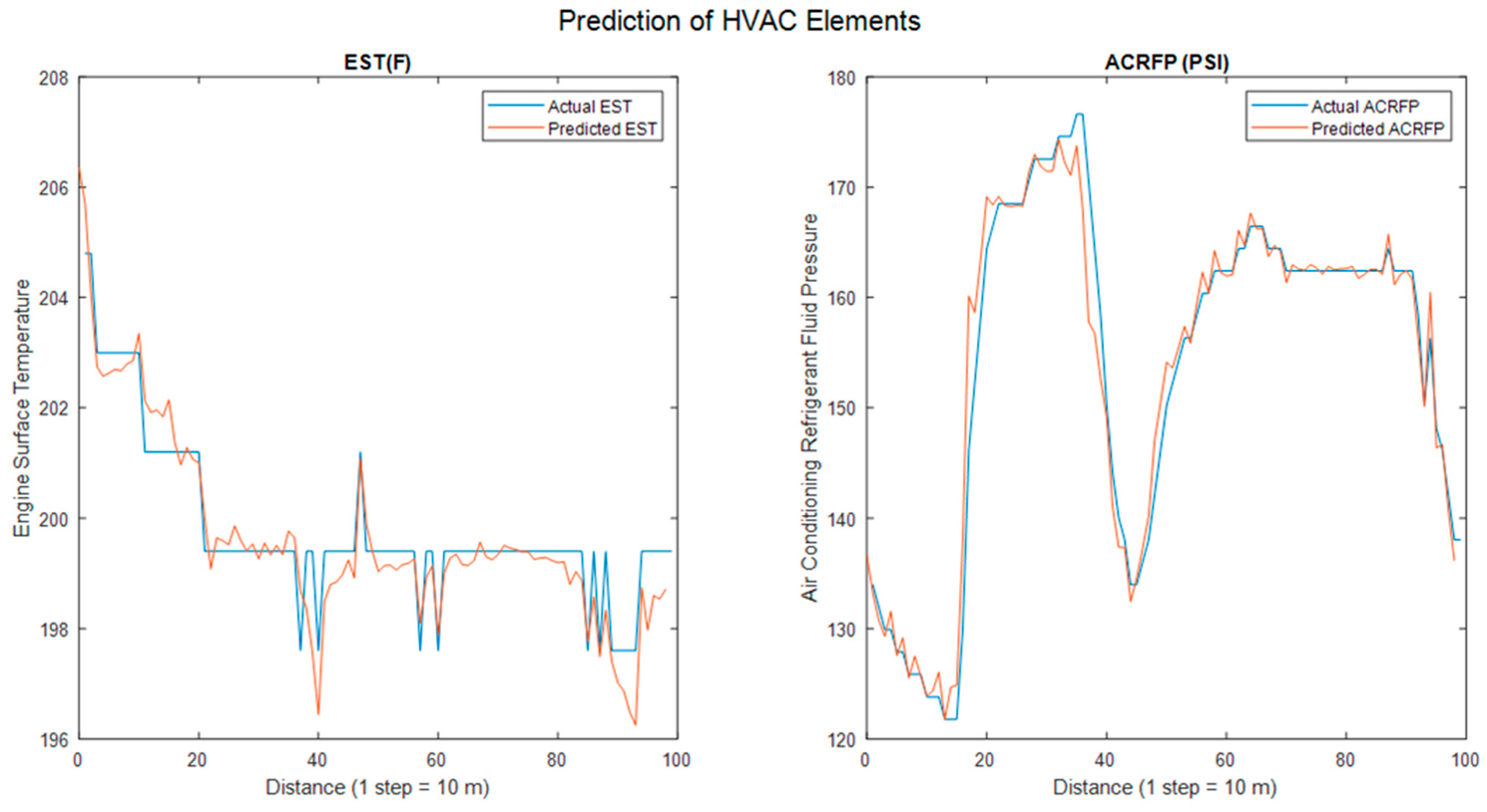
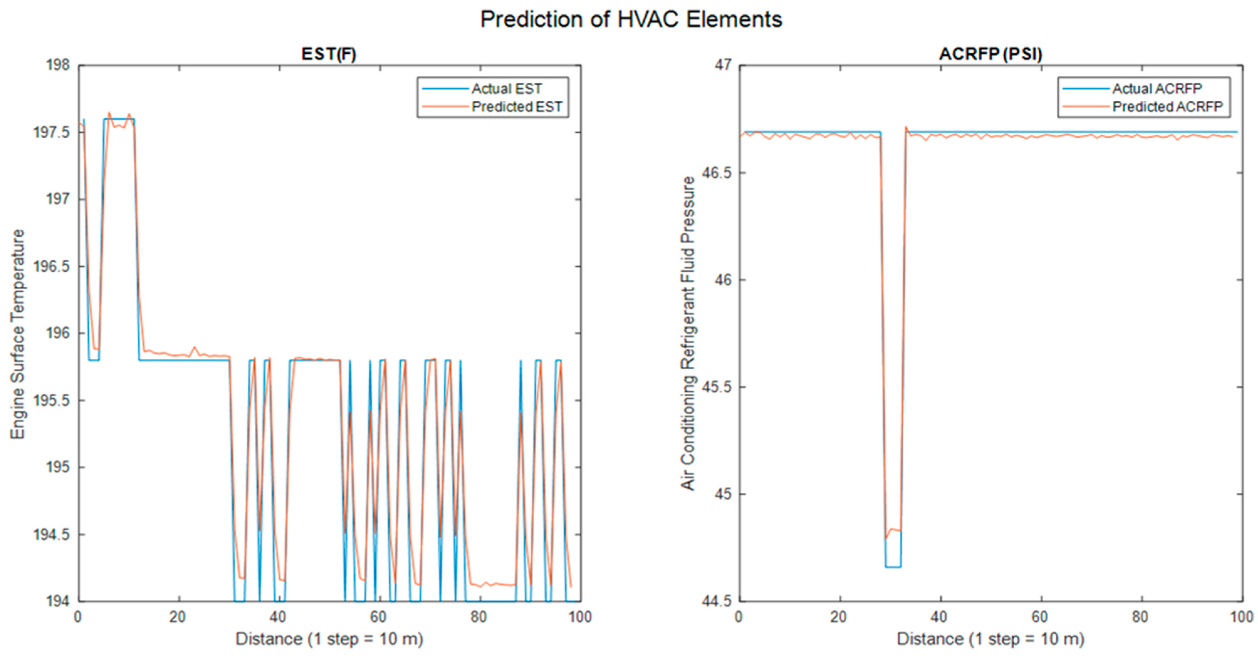
The test cases with ACCSSP > 25 MPH were selected, and individual training networks were developed for the two CATOP—elements. The results are shown in Figures S1–S5 for EAT > 65 °F and Figures S6–S10 for EAT < 45 °F for ACCSSP = [35 75] MPH. Each figure consists of two parts, EST (left) and ACRFP (right). Furthermore, each plot compares the measured data (blue) with the predicted values (orange). Finally, we validated the DL model using the statistical measures (RMSE, FOD, SNR) by comparing the actual and predicted values of CATOP, reported in

Table 7. NARX Model Performance—ACC Speeds [35 75] MPH.

(Date: 16 June 2020)			Data Set 1: NARX—DL Model Validation (Predicted-Actual)
			EST (°F)			ACRFP (PSI)
ACCSSP (MPH)	CAT (°F)	EAT (°F)	RMSE	FOD	SNR	RMSE	FOD	SNR
35	66	83.309	2.2057	1.5868	5.1067	14.0017	10.5611	16.1348
45	65	80.375	1.8169	1.4288	7.1183	10.8150	7.4388	12.1116
55	68	82.526	1.4794	1.0503	5.2231	9.5438	7.2012	20.3788
65	67	81.32	1.66	1.2953	12.7934	3.7248	2.7151	6.9461
75	70	86.081	1.2763	0.7945	5.7699	8.6413	5.2471	28.3001
(Date: 25 February 2021)			Data Set 2: NARX—DL Model Validation (Predicted-Actual)
			EST (°F)			ACRFP (PSI)
ACCSSP (MPH)	CAT (°F)	EAT (°F)	RMSE	FOD	SNR	RMSE	FOD	SNR
35	76	36.374	0.9528	0.6636	3.4284	2.9186	0.9376	1.3323
45	71	39.047	0.5678	0.3981	6.2342	0.0281	0.0148	1.7795
55	73	33.8	0.3916	0.2618	5.4806	0.0040	0.0007	0.3951
65	74	37.4	0.3080	0.2158	15.4239	0.0013	0.0007	1.3281
75	75	37.4	0.4556	0.3179	32.7227	0.0011	0.000	0.000

. The following Figure 6 and Figure 7 depict an example of a prediction of CATOP vector for the snippet ACCSSP = 70 MPH.

5.3. Estimation of CAT

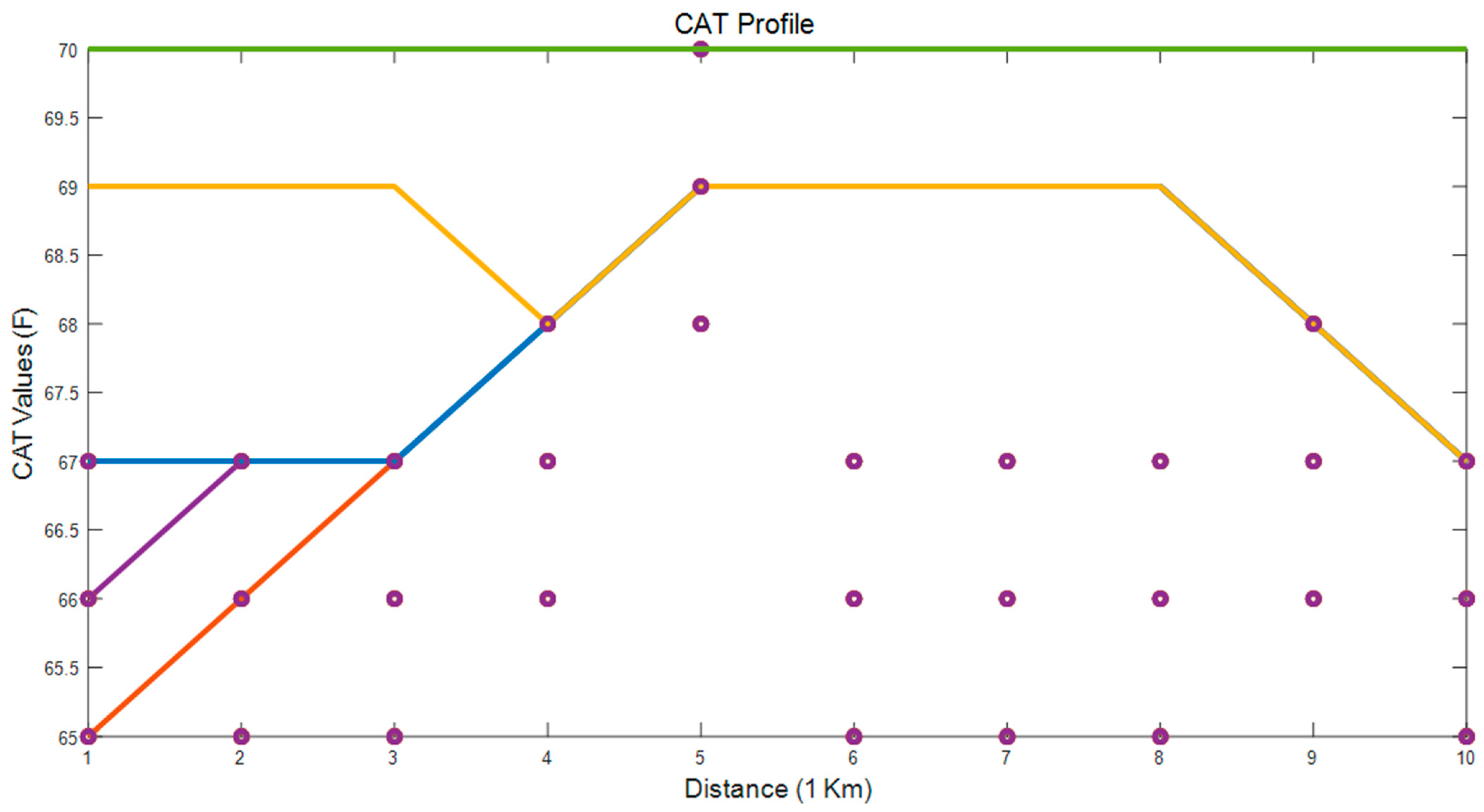
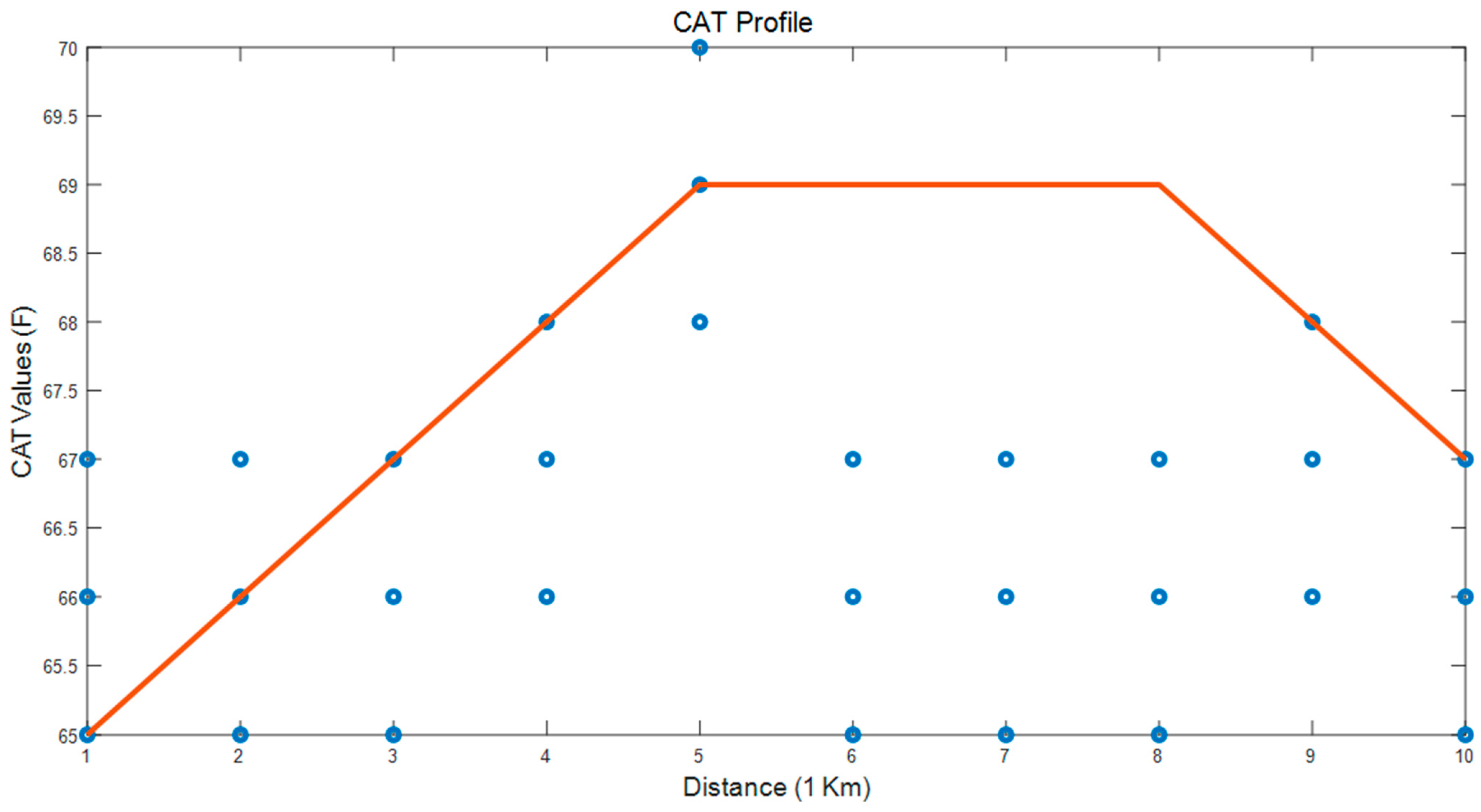
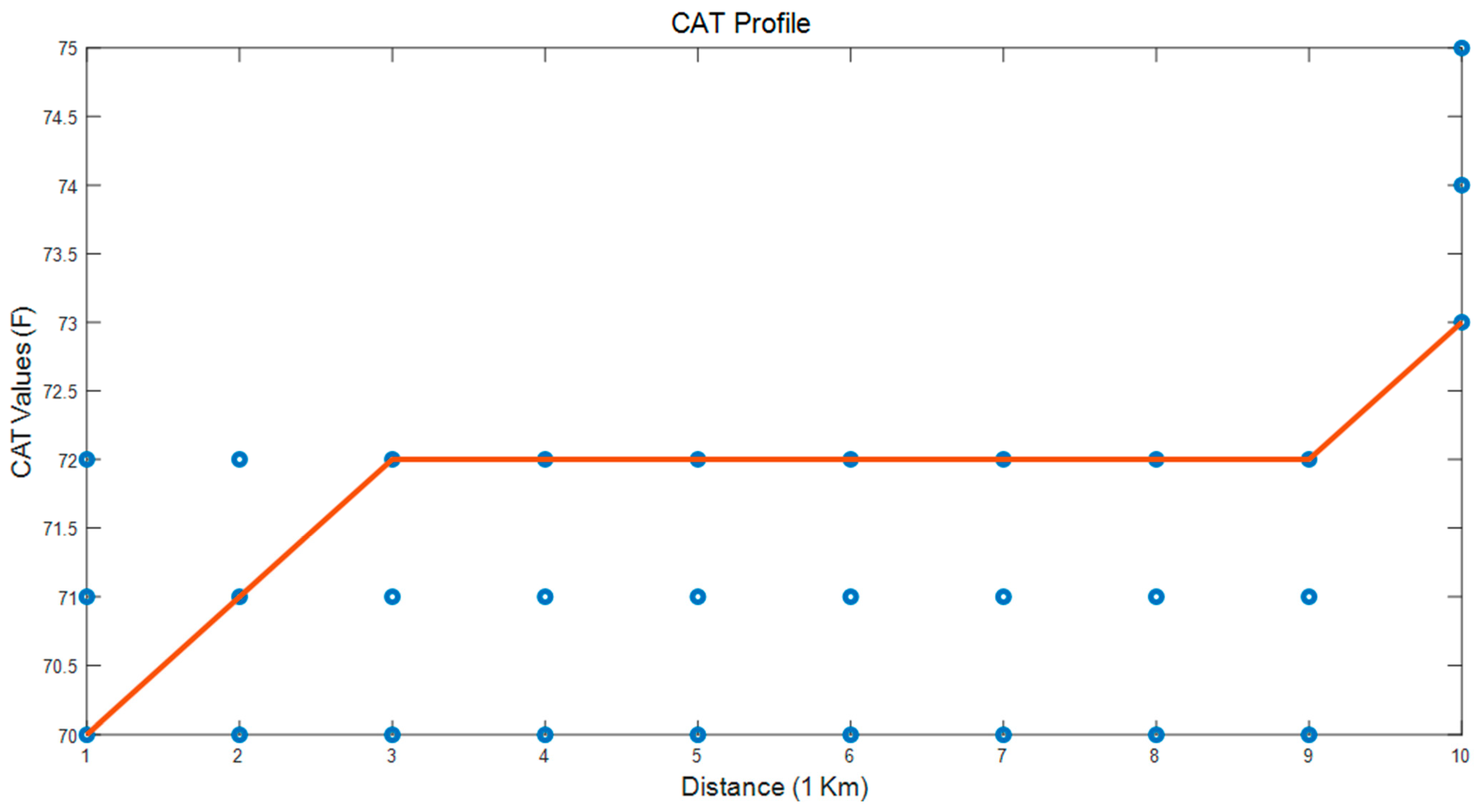
The analysis is conducted on the datasets retrieved using steps mentioned in Section 4. The snippet with ACCSSP = 70 MPH, with EAT = 78.75 °F and EAT = 38.3 °F, is applied with Steps 1–3, and the results are shown in Table 2, Table 3, Table 4 and Table 5. We varied the range of initial CAT with the default values, and Figure 8 and Figure 9 depict the possible CAT profiles resulting from Step 4. Therefore, constant initial CAT = 65 °F and 70 °F results in unique CAT profiles shown in Figure 10 and Figure 11. Similarly, the performance analysis for the test cases is shown in

Table 8. Performance analysis—Prediction of CAT.

Parameter	EAT (°F)	CAT Profile (°F)	Area	Conformance	${\mathit{R}}^2$	$\mathbf{Adj}{\mathit{R}}^2$	SSE	RMSE
ACCSSP = 35 MPH
EST [A1, A2]	78.566	66	515.975	−9.312	0.960	0.900	2.981	0.276
		Predicted	506.662		0.810	0.526	22.762	0.762
	36.806	74	424.360	4.411	0.989	0.973	12.604	0.567
		Predicted	428.771		0.992	0.980	11.889	0.551
ACRFP (B)	78.566	66	1957.947	−20.879	0.985	0.962	732.229	4.323
		Predicted	1937.067		0.983	0.958	810.917	4.550
	36.806	74	28,924.676	−4.548	0.982	0.954	1.384	0.188
		Predicted	28,920.127		0.985	0.962	1.121	0.169
ACCSSP = 45 MPH
EST [A1, A2]	71.384	65	350.128	−54.605	0.974	0.934	11.985	0.553
		Predicted	295.523		0.981	0.952	8.216	0.458
	33.8	71	8.335	−4.436	0.997	0.994	0.000	0.000
		Predicted	3.898		0.984	0.959	0.002	0.007
ACRFP (B)	71.384	65	968.488	259.626	0.915	0.788	845.487	4.646
		Predicted	1228.114		0.977	0.944	491.012	3.540
	33.8	71	29,057.213	0.462	0.998	0.996	0.000	0.000
		Predicted	29,057.675		0.887	0.717	0.000	0.002
ACCSSP = 55 MPH
EST [A1, A2]	70.997	65	658.373	−72.241	0.969	0.922	4.957	0.356
		Predicted	586.131		0.969	0.924	5.472	0.374
	33.8	73	307.908	−1.912	0.967	0.917	1.839	0.217
		Predicted	305.996		0.965	0.913	1.867	0.218
ACRFP (B)	70.997	65	2928.211	−229.571	0.970	0.925	2745.421	8.371
		Predicted	2698.639		0.974	0.936	2679.109	8.270
	33.8	73	28,850.426	−2.175	0.999	0.998	0.000	0.000
		Predicted	28,848.251		0.997	0.993	0.000	0.001
ACCSSP = 65 MPH
EST [A1, A2]	81.095	67	505.586	−31.343	0.978	0.944	7.887	0.449
		Predicted	474.242		0.948	0.871	22.979	0.766
	37.4	72	568.740	4.009	0.970	0.924	1.279	0.181
		Predicted	572.750		0.968	0.921	1.292	0.182
ACRFP (B)	81.095	67	3078.741	269.982	0.946	0.865	61.282	1.251
		Predicted	3348.724		0.961	0.901	92.636	1.538
	37.4	72	28,851.571	0.180	0.912	0.779	0.000	0.000
		Predicted	28,851.752		0.989	0.971	0.000	0.000
ACCSSP = 75 MPH
EST [A1, A2]	84.4	68	639.694	246.732	0.952	0.880	7.089	0.425
		Predicted	886.427		0.952	0.879	28.418	0.852
	37.40	70	669.610	−5.7879	0.966	0.915	2.408	0.248
		Predicted	663.822		0.967	0.917	2.350	0.245
ACRFP (B)	84.4	68	2231.887	−782.45	0.919	0.797	383.320	3.128
		Predicted	1449.436		0.909	0.773	1664.53	6.518
	37.4	70	28,850.316	0.065	0.999	0.996	0.000	0.000
		Predicted	28,850.381		0.925	0.813	0.000	0.000

, and the plots of the CAT profiles are shown in Figures S11–S20.

6. Discussion

In this research, the predictive model of CAT, one of the elements of DBV, is proposed. This article involved multiple concepts, developing the NARX DL model by mapping the elements VLV and CATOP (Section 2.1), defining the optimal HVAC criteria, predicting optimal CAT, and detailed validation using various test cases.

The properties of the NARX DL model are defined in Table S1, and its efficacy to predict CATOP vectors is validated using statistical techniques (RMSE, FOD, SNR), shown in Table 7. The test cases were developed with ACCSSP = [35 75] MPH for the two datasets differentiated by EAT > 65 °F and <45 °F. The EST RMSE < 2.2 for set 1 and <0.95 for set 2, whereas ACRFP FOD < 11 for set 1 and <0.94 for set 2. In real-time, the values of [EST (°F), ACRFP (PSI)] are always fluctuating, and hence the resulting SNR values are <17 for all cases, which depict acceptable noise. Despite the stochastic variation of the data, by visualising Figure 6 and Figure 7 and Figures S1–S10, we observed that the predicted values fit the real-time curves. It is a well-known fact that extended training with multiple data sets would enhance the performance of the NARX DL model. Also, this article proposes the core concept of predicting the CAT profile by optimising CATOP elements. Therefore, the DL model is developed using default training properties and is assumed to produce acceptable results. Thus, we initiate the further steps of the project.

We selected the snippet with ACCSSP = 70 MPH to initiate the testing, and the proposed methodology described in steps 4.1–4.4 (Figure 4) is adapted. The required input sets for the iterative analysis are generated using the equations defined in Table 1, and sample input sets are shown in Table 2. The optimal HVAC criteria proposed in Section 3 and Table 3 and Table 4 are developed for estimating optimal CAT values for 10 steps = 100 m. Thus, an optimal CAT matrix is developed shown in Table 5, executing the algorithm described in Section 4.4, and optimal CAT profiles are generated shown in Figure 8 and Figure 9. Therefore, by fixing the initial value of CAT, a unique CAT profile has resulted, as shown in Figure 10 and Figure 11.

To validate the proposed methodology, we developed the input sets with constant and predicted CAT profiles (Figures S11–S20), and these sets are fed into the NARX DL model. The results of the performance analysis comparing the constant and predicted CAT profiles are shown in Table 8. The test case with ACCSSP = 75 MPH, EAT = 84.4 °F, resulted in higher EST = 246.73 (°F) for constant CAT = 68 °F and predicted CAT profile has lower ACRFP = 782.45 (PSI). Whereas for EAT = 37.4 °F, the predicted CAT has EST lower by 5.787 (°F), and ACRFP has similar performance. The snippet with ACCSSP = 45 MPH, EAT = 71.384 °F, resulted in ACRFP lowering by 259.626 (PSI) for constant CAT = 65 °F, which is deviating the proposed concept, but the smoothness performance for predicted CAT has higher [$R^2$, Adj $R^2$] = [0.977 0.944] and lower [SSE RMSE] = [491.01 3.540]. It is easy to see that the performance of the predicted CAT profile with test case ACCSSP = 55 MPH has enhanced performance for all the parameters, and a similar explanation follows for the rest of the scenarios.

Therefore, the predicted CAT outperforms the constant CAT in maintaining the EST closer to 194 °F and ACRFP in the range of the threshold defined in Figure 3 [25] and Table S2. This approach satisfies the optimal HVAC criteria, and this enhances the EOC.

7. Conclusions and Future Work

In real-time, the DBV is defined by the three elements (Speeding, Steering, CAT), and variation of these parameters is the user’s prerogative. In this manuscript, we proposed a new methodology to input the range of CAT and predict the optimal CAT profile, which could augment the HVAC functionality. The criteria of optimal HVAC were empirically developed using the elements (EST, ACRFP) predicted by the NARX DL model by mapping the elements VLV. We validated the NARX DL model by using real-time datasets and applied statistical techniques to the conformance of predicted and actual values.

The unique CAT profile was generated in the user-defined range, satisfying the constraints of optimal HVAC criteria. We prepared new input sets with the predicted and constant CAT profiles and fed them into the NARX DL model, which validates the predicted (EST, ACRFP) in the optimal desired range. The computational results obtained are satisfactory, and we quantified short snippets of distance (1 × 10³ m) for the speed ranges ACCSSP = [25 85] MPH. Also, the DL model generated smoother CAT profiles, and this method could derive a new functionality of inputting a range of user-defined set CAT to the HVAC system to enhance vehicle performance.

In this research, environmental factors (traffic congestion, solar reception (idling), HUM, ATP), HVAC parameters (compressor load, engine fan speed, power consumed), and human comfort elements (cabin moisture, multiple CAT inputs, psychrometric analysis) were not considered in the NARX DL model because of minimal variations and unavailability of the CAN data retrieved. Also, this project is confined to a single-vehicle test, that is, a 2020 Cadillac CT5 provided by GMC, and future work would involve developing the model to include all the affecting parameters and extend the validation using multiple vehicle test cases.

References

1. Holweg, M. The evolution of competition in the automotive industry. In Build to Order; Springer: London, UK, 2008; pp. 13–34. [Google Scholar]
2. Farrington, R.; Rugh, J. Impact of Vehicle Air-Conditioning on Fuel Economy, Tailpipe Emissions, and Electric Vehicle Range (No. NREL/CP-540-28960); National Renewable Energy Lab: Golden, CO, USA, 2000.
3. Khayyam, H.; Kouzani, A.Z.; Hu, E.J.; Nahavandi, S. Coordinated energy management of vehicle air conditioning system. Appl. Therm. Eng. 2011, 31, 750–764. [Google Scholar] [CrossRef]
4. Johnson, V.H. Fuel Used for Vehicle Air Conditioning: A State-by-State Thermal Comfort-Based Approach (No. 2002-01-1957); SAE Technical Paper; SAE International: Warrendale, PA, USA, 2002. [Google Scholar]
5. Lee, J.; Kim, J.; Park, J.; Bae, C. Effect of the air-conditioning system on the fuel economy in a gasoline engine vehicle. Proc. Inst. Mech. Eng. Part D J. Automob. Eng. 2013, 227, 66–77. [Google Scholar] [CrossRef]
6. Khayyam, H. Adaptive intelligent control of vehicle air conditioning system. Appl. Therm. Eng. 2013, 51, 1154–1161. [Google Scholar] [CrossRef]
7. Nasution, H. Development of fuzzy logic control for vehicle air conditioning system. Telkomnika 2008, 6, 73. [Google Scholar] [CrossRef] [Green Version]
8. Khayyam, H.; Abawajy, J.; Jazar, R.N. Intelligent energy management control of vehicle air conditioning system coupled with engine. Appl. Therm. Eng. 2012, 48, 211–224. [Google Scholar] [CrossRef]
9. Khayyam, H.; Kouzani, A.Z.; Hu, E.J. Reducing energy consumption of vehicle air conditioning system by an energy management system. In Proceedings of the 2009 IEEE Intelligent Vehicles Symposium, Xi’an, China, 3–5 June 2009; pp. 752–757. [Google Scholar]
10. Huang, K.D.; Tzeng, S.C.; Jeng, T.M.; Chiang, W.D. Air-conditioning system of an intelligent vehicle-cabin. Appl. Energy 2006, 83, 545–557. [Google Scholar] [CrossRef]
11. Fayazbakhsh, M.A.; Bahrami, M. Comprehensive Modeling of Vehicle Air Conditioning Loads Using Heat Balance Method; SAE Technical Paper; SAE International: Warrendale, PA, USA, 2013; Volume 2013, p. 1507. [Google Scholar]
12. Cvok, I.; Ratkovic, I.; Deur, J. Optimization of Control Parameters of Vehicle Air-Conditioning System for Maximum Efficiency (No. 2020-01-1242); SAE Technical Paper; SAE International: Warrendale, PA, USA, 2020. [Google Scholar]
13. Kolachalama, S.; Malik, H. Predictive Model of Adaptive Cruise Control Speed to Enhance Engine Operating Conditions. Vehicles 2021, 3, 749–763. [Google Scholar] [CrossRef]
14. Kolachalama, S.; Lakshmanan, S. Using Deep Learning to Predict the Engine Operating Point in Real-Time (No. 2021-01-0186); SAE Technical Paper; SAE International: Warrendale, PA, USA, 2021. [Google Scholar]
15. Wang, W.; Xi, J.; Chen, H. Modeling and recognizing driver behavior based on driving data: A survey. Math. Probl. Eng. 2014, 2014, 1–20. [Google Scholar] [CrossRef] [Green Version]
16. Kolachalama, S.; Kuppa, K.; Mattam, D.; Shukla, M. Thermal Analysis of Radiator Core in Heavy Duty Automobile. In Proceedings of the Heat Transfer Summer Conference, Jacksonville, FL, USA, 10–14 August 2008; Volume 48487, pp. 123–127. [Google Scholar]
17. Eathakota, V.; Singh, A.K.; Kolachalam, S.; Krishna, K.M. Determination of optimally stable posture for force actuator based articulated suspension for rough terrain mobility. In Proceedings of the FIRA RoboWorld Congress, Bangalore, India, 15–17 September 2010; Springer: Berlin/Heidelberg, Germany, 2010; pp. 154–161. [Google Scholar]
18. Talom, H.L.; Beyene, A. Heat recovery from automotive engine. Appl. Therm. Eng. 2009, 29, 439–444. [Google Scholar] [CrossRef]
19. Yan, X.; Fleming, J.; Lot, R. A/C energy management and vehicle cabin thermal comfort control. IEEE Trans. Veh. Technol. 2018, 67, 11238–11242. [Google Scholar] [CrossRef]
20. Roberts, A.; Brooks, R.; Shipway, P. Internal combustion engine cold-start efficiency: A review of the problem, causes and potential solutions. Energy Convers. Manag. 2014, 82, 327–350. [Google Scholar] [CrossRef] [Green Version]
21. Borman, G.; Nishiwaki, K. Internal combustion engine heat transfer. Prog. Energy Combust. Sci. 1987, 13, 1–46. [Google Scholar] [CrossRef]
22. Autozone: Air Conditioning Pressure Chart; R134a-Refrigerant; California Air Ressources Board (CARB): Sacramento, CA, USA, 2009.
23. Kolachalama, S.; Hay, C.L.; Mushtarin, T.; Todd, N.; Heitman, J.; Hermiz, S. An Algorithm to Estimate Steering Behavior Using Vehicle Radius Of Curvature, 647068, Research Disclosure; Questel Ireland Ltd.: Paris, France, 2018. [Google Scholar]
24. Xing, W.; Chen, H.; Ding, H. The application of controller area network on vehicle. In Proceedings of the IEEE International Vehicle Electronics Conference (IVEC’99)(Cat. No. 99EX257), Changchun, China, 9 September 1999; pp. 455–458. [Google Scholar]
25. Gallardo, F.B. Extraction and Analysis of Car Driving Data Via OBD II. Ph.D. Thesis, Miguel Hernández University of Elche, Alicante, Spain, 2018. [Google Scholar]
26. Benmimoun, M.; Pütz, A.; Zlocki, A.; Eckstein, L. Effects of acc and fcw on speed, fuel consumption, and driving safety. In Proceedings of the 2012 IEEE Vehicular Technology Conference (VTC Fall), Quebec City, QC, Canada, 3–6 September 2012; pp. 1–6. [Google Scholar]
27. Eathakota, V.P.; Kolachalama, S.; Krishna, K.M.; Sanan, S. Optimal posture control for force actuator based articulated suspension vehicle for rough terrain mobility. In Advances in Mobile Robotics; World Scientific: Coimbra, Portugal, 2008; pp. 760–767. [Google Scholar]
Figure 1. Heat exchange: Vehicle interactive elements.
Vehicles 03 00052 g001
Figure 2. NARX DL Model—Inputs and Outputs [13].
Vehicles 03 00052 g002
Figure 3. R134a ACS—ACRFP threshold curve.
Vehicles 03 00052 g003
Figure 4. Prediction of CAT—Process [13].
Vehicles 03 00052 g004
Figure 5. Path traversed—2020 Cadillac CT5 [Source: Google maps].
Vehicles 03 00052 g005
Figure 6. Prediction of CATOP—ACCSSP = 70 MPH; CAT = 68 °F; EAT = 78.75 °F.
Vehicles 03 00052 g006
Figure 7. Prediction of CATOP—ACCSSP = 70 MPH; CAT = 72 °F; EAT = 40.1 °F.
Vehicles 03 00052 g007
Figure 8. ACCSSP = 70 MPH; CAT = [65 70] °F; EAT = 78.75 °F.
Vehicles 03 00052 g008
Figure 9. ACCSSP = 70 MPH; CAT = [70 75] °F; EAT = 38.3 °F.
Vehicles 03 00052 g009
Figure 10. ACCSSP = 70 MPH; Initial CAT = 65 °F; EAT = 78.75 °F.
Vehicles 03 00052 g010
Figure 11. ACCSSP = 70 MPH; Initial CAT = 70 °F; EAT = 38.3 °F.
Vehicles 03 00052 g011