Context-Aware Sensor Uncertainty Estimation for Autonomous Vehicles

Abstract

Sensor uncertainty significantly affects the performance of autonomous vehicles (AVs). Sensor uncertainty is predominantly linked to sensor specifications, and because sensor behaviors change dynamically, the machine learning approach is not suitable for learning them. This paper presents a novel learning approach for predicting sensor performance in challenging environments. The design of our approach incorporates both epistemic uncertainties, which are related to the lack of knowledge, and aleatoric uncertainties, which are related to the stochastic nature of the data acquisition process. The proposed approach combines a state-based model with a predictive model, where the former estimates the uncertainty in the current environment and the latter finds the correlations between the source of the uncertainty and its environmental characteristics. The proposed approach has been evaluated on real data to predict the uncertainties associated with global navigation satellite systems (GNSSs), showing that our approach can predict sensor uncertainty with high confidence.

1. Introduction

Developments in mobility technology arise from the need to achieve greater independence and safety in ambiguous or challenging situations. The latest revolution in transportation is fully autonomous vehicles (AVs), which are equipped with advanced sensor technology, smart controllers, and intelligent actuators with the aim of providing a hassle-free driving experience for passengers and road users. Furthermore, complex algorithms and communication technologies integrated into autonomous driving systems, such as path planners, path trackers, and object detectors, help vehicles plan, analyze, and make appropriate decisions in their environments.

Nevertheless, uncertainty greatly hinders the adoption of AVs in real life. The complexity and natural behavior of the related built-in technologies lead to large errors and ambiguities in all vehicle subsystems. For example, this can be observed under adverse weather conditions: visual sensors cannot collect sufficient valuable information in rain or snow. The subsystems in AVs completely depend on measurements obtained by onboard sensors, including global navigation satellite systems (GNSSs), inertial measurement units (IMUs), cameras, and light detection and ranging (LiDAR) sensors, which are highly susceptible to varying environmental conditions as well as road features and geometries. Noisy data can lead to unsafe behavior and potential traffic accidents. Therefore, to allow vehicles to operate safely in the real world and reduce the ambiguity of sensor measurements, the associated errors require careful handling. Several attempts have been made to address this issue. For instance, some authors (e.g., [1]) have fused multiple sensor readings to enhance the performance of the navigation system in uncertain situations. Other authors (see [2,3]) tackled the uncertainty issue using path planning approaches. However, the aleatoric uncertainty, which is related to the quality of the sensors and their measurement accuracy, is strongly correlated with the environmental conditions, and this correlation has been overlooked by the previous works. A thorough literature review of uncertainty-handling approaches is given in Section 2.

With attention to residual correction, the Kalman filter is widely utilized as a state-based model and is highly appropriate for modeling the major random processes affecting AVs. In particular, GNSS readings are often far off the actual values. Through the incorporation of other sensor readings (i.e., sensor fusion), such as IMU signals, the Kalman filter is capable of correcting these innovations. One major limitation of this approach, however, is that such a state estimation procedure fails to predict the source of the uncertainty; consequently, the vehicle may not be warned about challenging conditions such that it can act to avoid a crash. Suitable analysis of the driving environment might yield valuable contextual information about the degraded sensor performance. Such information could potentially allow the sensor uncertainty to be modeled using machine learning.

Machine learning models endow AVs with intelligent functions. These models enable AVs to collect massive amounts of data from their environments using sensors, analyze those data, and ultimately make correct decisions accordingly. These models can learn to perform tasks as efficiently as humans. In such a way, machine learning can replace traditional techniques, making it competent for a wide range of AV functions such as object detection, classification, and segmentation. One powerful type of model, called a Bayesian neural network, is a hybrid of a deep neural network (DNN) and a probabilistic model, combining the flexibility of DNNs with the ability to estimate the uncertainty of its predictions.

The aim of the research presented in this paper is to understand how the uncertainty that arises under challenging conditions affects AV models and data, that is, how uncertainty from different sources influences model estimation. An end-to-end predictive approach for the sensor uncertainty of an AV is presented. A Kalman filter outputs the sensor uncertainty for each sensor on each road segment. These uncertainties are then correlated with the environmental and road features to predict sensor behaviors in future similar scenarios. This approach can be used to obtain an estimate of the sensor quality in any given space. The presented technique can be generalized and adapted to any driving subsystem to improve its quality. For instance, the resultant sensor uncertainty estimates can be incorporated into a path planner to avoid high-risk road segments.

In brief, the main contributions of this paper are as follows.

• To handle sensor uncertainty in AVs, an end-to-end context-aware approach is proposed that takes advantage of both Kalman filtering and machine learning and allows for both epistemic and aleatoric uncertainties.
• An evaluation of the proposed approach is performed using real data, and the results reveal that our approach can estimate the sensor uncertainty with a low margin of error.

The rest of this paper is organized as follows. Section 2 reviews related works. Section 3 introduces the proposed method. Section 4 presents experimental results to illustrate and validate the theoretical findings. Finally, Section 5 offers conclusions and perspectives on future work.

2. Related Works

Sensor uncertainty can affect all of a vehicle’s measurements, including the estimated positions and velocities of the vehicle itself or other surrounding objects. This uncertainty results in noisy measurements. The literature contains three approaches to cope with sensor uncertainty: data fusion, path planning, and machine learning.

2.1. Data Fusion Approaches

Data fusion is an effective tool to cope with the uncertainties arising from noisy measurements and nonlinear multimodality; thus, it has been extensively applied to address sensor uncertainty [4]. A data fusion strategy involves combining and transforming homogeneous or heterogeneous data into a uniform configuration. Commonly, such a strategy is exploited to estimate the optimal state. Such manipulation has enabled crucial advances in various navigation and intelligence-demanding tasks, such as perception [1,5,6,7,8], object detection and tracking [9,10,11,12,13,14], semantic segmentation [15,16,17,18,19,20,21], and control [22,23,24] for AVs.

Different approaches have been leveraged to fuse multisensor data, among which fuzzy logic, Kalman filtering, and machine learning offer the best capabilities in addressing this issue and thus are widely adopted. Unlike other sensor fusion techniques, fuzzy logic systems provide a clear interpretation of their operations or decisions since they represent information in the form of rules that mimic human reasoning. Moreover, such systems can accommodate data of various degrees of quality, including vague, distorted, and imprecise data. However, fuzzy systems depend entirely on domain knowledge, which might not be available. The Kalman filter is the most practical state estimator due to its optimality and structure. However, the basic Kalman filter requires that both the system and observation models consist of linear equations, which is not realistic in many applications. To allow nonlinear problems to be solved in this way, these problems can be sliced into linear pieces that can be effectively addressed by the Kalman filter. This variant is called the extended Kalman filter (EKF). The EKF approach has been proven to demonstrate improved performance in AV tasks compared to other approaches because it offers the ability to calculate and correct for residuals. Both Kalman filtering and fuzzy logic require little memory space and few CPU resources. Machine learning can also offer quick outcomes but requires careful design and extensive training and validation processes.

2.2. Path Planning Approaches

Another way to handle uncertainty in AVs is path planning, in which routes are computed with the objective of reducing uncertainty. Recently, attention has been focused on low-uncertainty path planning since paths planned in this way offer safe navigation for both vehicle passengers and other road users. Researchers have primarily utilized three methodologies to address low-uncertainty path planning: partially observed Markov decision processes (POMDPs) [2], linear quadratic Gaussian (LQG) control, and fuzzy logic. POMDP-based planners formulate the problem as a belief space in which every possible uncertain belief (over states) is mapped to actions. A POMDP policy encodes a plan to achieve the maximum reward. The literature contains exact solutions for problems with both finite [25] and infinite [26] horizons. However, because they consider a continuous belief space, these planners consume considerable computational resources, affecting their scalability. To alleviate the scalability issue, many approximation-based or sample-based methods for solving POMDPs have been proposed, such as probabilistic roadmaps (PRMs) [27] and rapidly exploring random trees (RRTs) [28]. These planners have been proven as highly competent in terms of motion planning in high-dimensional spaces; see, e.g., [29,30,31,32,33,34,35]. Instead of utilizing an explicit representation, sample-based planners depend on a collision checking component, which determines the feasibility of candidate trajectories, to construct a belief graph (roadmap). However, the existing sample-based planners can only tackle problems for which the size of the state space is limited to at most a few thousand states.

An alternative planning approach is to construct a belief space using the LQG estimator, which provides an optimal estimate of the state of a linear system with additive Gaussian noise [3]. An LQG-based planner requires the generation of an initial trajectory, for which two common architectures have been proposed. The first architecture is divided into a trajectory process and control policies. An instance of this architecture was presented in [36], where candidate paths generated using RRT and LQG outputs were evaluated over each path. One major drawback of this approach is that an optimal trajectory might not be found because the path optimality is determined based on a minimum cost that is restricted to a bounded collision belief. One resolution to this issue is to use a local LQG approach to estimate the belief over the trajectories formed by the candidate paths and improve these paths using incremental sampling refinement [37]. The second architecture employs an iterative distinct routine that combines the trajectory process and control policies [38,39]. However, AV systems are complicated, dynamic, and nonlinear. As a result, simple distributions such as the Gaussian distribution cannot effectively model and represent beliefs about sensor uncertainties. Moreover, although stochastic approaches can resolve the relevant computational complexity and provide reasonable outcomes, optimal solutions are not always guaranteed.

Low-uncertainty path planning can exploit fuzzy logic to model uncertainty. One recent work has proposed a collaborative fuzzy logic-based path planning approach that models sensor uncertainty and computes paths with the minimum uncertainty [40]. The authors demonstrated that vehicles could successfully maneuver along road segments with uncertainty sources using this planning approach. However, this approach requires domain knowledge to configure the fuzzy logic models, including the environmental factors influencing the quality of sensor readings, which might be challenging to obtain. Thus, there is an urgent need to enable AVs to understand their sensing limitations and act accordingly. A better understanding of a vehicle’s sensing capabilities will facilitate the prediction of sources of sensor uncertainty.

2.3. Machine Learning Approaches

Predictions can be readily obtained using machine learning models such as DNNs, which can capture nonlinear relations within high-dimensional data. DNNs are typically trained using maximum likelihood (ML) or maximum a posteriori (MAP) estimators. Thus, such a predictive model yields prediction value(s) but does not provide information about the underlying uncertainty. It is crucial to characterize a model’s confidence about its predictions, especially for applications such as AVs, which commonly encounter life-threatening situations [41]. Therefore, a probabilistic variant of a DNN with an uncertainty estimation functionality has been proposed, inspired by Bayesian statistics [42,43,44]. The network parameters (i.e., weights) of a Bayesian neural network (BNN) have an arbitrary prior distribution, and the posterior distribution is then computed. Because of their large numbers of parameters and intractable posterior distributions, BNNs are resource-intensive models. Thus, an approximate inference approach should be applied. Variational inference is a popular approximation approach in which the differences between the distribution parameters and the true distribution are typically optimized by minimizing the Kullback–Leibler (KL) divergence [45,46]. Although BNNs serve best as supervised learning models, obtaining sufficient labeled data is very challenging. Thus, a new approach is needed for estimating sensor uncertainties and modeling them for future prediction.

3. Method

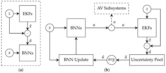
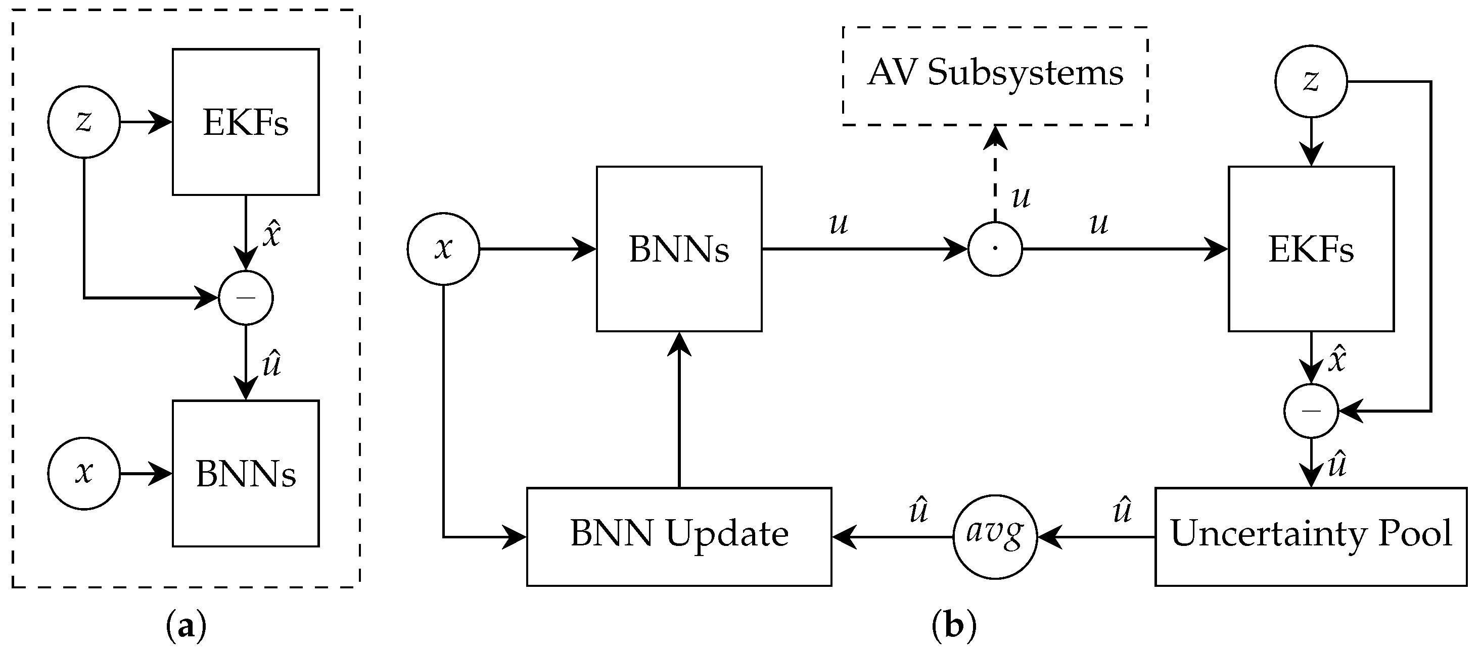
The underlying aim of our approach is to enable cooperation between a Kalman filter and a machine learning model to estimate sensor uncertainty in a particular road segment. There are many possible Kalman filter variants and machine learning models other than those proposed in this paper. However, the results of our experiments demonstrate highly reliable outcomes overall when following the method detailed below. The proposed method includes three primary components: an ensemble-based Kalman filter, a sensor uncertainty estimator, and a BNN model. Figure 1 presents an overview of the proposed method.

3.1. Ensemble-Based Kalman Filter

The Kalman filter is a powerful and practical estimator that is adopted in many AV systems, such as controllers, localization and mapping systems, and object trackers. The basic Kalman filter can generate estimates only for models described in terms of linear relationships. However, the sensor data collected by AVs are nonlinear; therefore, for such a filter to be used, the corresponding models must be decomposed into linear components. To assimilate these complex data, this work employs the EKF, which associates states with a measurement or observation space using nonlinear functions. The EKF consists of two stages: prediction and correction. The filter is first initialized with a state $x_0$ with error covariance $P_0$. In the prediction stage, the state and the error covariance are projected forward as expressed by the following equations:

$${\widehat{x}}_{k+1|k}\approx f({\widehat{x}}_{k+1|k},u_k),$$

(1)

$$P_{k+1|k}=F_k{P}_{k|k}{F}_k^T+Q_k,$$

(2)

where $f(·)$ is a nonlinear model of the state transition dynamics, u is a control variable vector, Q is the process noise covariance matrix, and F is an approximation of $f(·)$ obtained using the first derivative of the Taylor series called the Jacobian matrix, which is defined as

$$F\equiv \left[\begin{array}{cccc}\frac{\partial f_1}{\partial x_1}& \frac{\partial f_1}{\partial x_2}& \cdots & \frac{\partial f_1}{\partial x_n}\\ ⋮& ⋮& \ddots & ⋮\\ \frac{\partial f_n}{\partial x_1}& \frac{\partial f_n}{\partial x_2}& \cdots & \frac{\partial f_n}{\partial x_n}\end{array}\right]$$

(3)

In the correction stage, the filter computes the optimal estimate by updating the initial estimate with a new sensor measurement z using the relative weight or Kalman gain K and also updates the error covariance.

$$K_k=P_{k|k-1}{H}_k{(H_k{P}_{k|k-1}{H}_k^T+R_k)}^{-1}$$

(4)

$${\widehat{x}}_{k|k}\approx {\widehat{x}}_{k|k-1}+K_k[z_k-h\left({\widehat{x}}_{k|k-1}\right)]$$

(5)

$$P_{k|k}=(I-K_k{H}_k)P_{k|k-1}$$

(6)

where $h(·)$ and H are functions that associate the vehicle’s state with the available observation space and its Jacobian, respectively, and R is the sensor noise covariance matrix or measurement error.

In this paper, the Kalman filter is utilized to perform the localization task using only one target sensor and another supporting sensor (i.e., an IMU). The purpose of the EKF is not to localize the vehicle as in standard applications; rather, it is to detect and quantify the variation between the optimal estimated position and the observed position. IMUs as supporting sensors are less susceptible to errors, and the relevant errors can be corrected through filtering. The filtering error for each road segment is stored for use in future uncertainty prediction. Given an estimate of the current position, velocity, and acceleration of the vehicle, the future vehicle motion can be predicted using the laws of motion (or a Newtonian prediction model). Thus, the state vector to be estimated for each movement is defined as:

$$h\left(x\right)={[x_m,y_m,{\omega }_m,s_m]}^T,$$

(7)

where $x_m$ and $y_m$ are the coordinates observed by sensor m, $\omega$ is the angular speed, and s is the speed at which the vehicle moves. The angular speed and the true speed can be calculated via the following equations:

$$\omega =\frac{d}{dt}{tan}^{-1}\left(\frac{\dot{y}}{\dot{x}}\right)=\frac{\dot{x}\ddot{y}-\dot{y}\ddot{x}}{{\dot{x}}^2+{\dot{y}}^2},$$

(8)

$$s=\sqrt{{\dot{x}}^2+{\dot{y}}^2},$$

(9)

where $\dot{x}$ and $\dot{y}$ are the first derivatives (i.e., velocity) of the vehicle’s movement in the x and y coordinates and $\ddot{x}$ and $\ddot{y}$ are the second derivatives (i.e., acceleration). Given the state vector function $h(·)$, the EKF linearizes the state transition matrix H by evaluating the Jacobian (Equation (10)) at the predicted state vector.

$$H_k=\frac{\partial h\left({\widehat{x}}_{k+1|k}\right)}{\partial {\widehat{x}}_{k+1|k}}.$$

(10)

Another adjustment worth mentioning is that in the prediction stage, the process noise covariance matrix, Q, incorporates the third derivatives (i.e., jerk) of the vehicle’s x and y positions (see Equation (11)) as Gaussian random variables with zero mean and variances of ${\sigma }_{\stackrel{⃛}{x}}^2$ and ${\sigma }_{\stackrel{⃛}{y}}^2$. These variances are typically unknown and thus are estimated from the historical data, as shown in Equation (12). Considering the vehicle’s jerk in Q enables the correction of errors caused by rapid acceleration changes, which are inevitable in AVs.

$$\begin{array}{cc}\hfill Q_k& =var\left({\left[\frac{\Delta t^3}{6}\stackrel{⃛}{x},\frac{\Delta t^2}{2}\stackrel{⃛}{x},\Delta t\stackrel{⃛}{x},\frac{\Delta t^3}{6}\stackrel{⃛}{y},\frac{\Delta t^2}{2}\stackrel{⃛}{y},\Delta t\stackrel{⃛}{y}\right]}^T\right)\hfill \\ \hfill & ={\sigma }_{\stackrel{⃛}{x}}^{2}var\left(\stackrel{⃛}{x}{\left[\frac{\Delta t^3}{6},\frac{\Delta t^2}{2},\Delta t,0,0,0\right]}^T\right)+{\sigma }_{\stackrel{⃛}{y}}^{2}var\left(\stackrel{⃛}{y}{\left[\frac{\Delta t^3}{6},\frac{\Delta t^2}{2},\Delta t,0,0,0\right]}^T\right)\hfill \end{array}$$

(11)

$${\sigma }_{\stackrel{⃛}{x}}^2={\sigma }_{\stackrel{⃛}{y}}^2=max\left(var\left({\stackrel{⃛}{x}}_{0:k}\right),var\left({\stackrel{⃛}{y}}_{0:k}\right)\right)$$

(12)

The sensor measurement vector, z, is designed to incorporate the noisy readings (x and y coordinates) that require filtering as measured by the target sensor. Reliable sensor signals such as velocity and acceleration are injected into the filtering process in the form of a control vector. The EKF estimates the optimal positions of the vehicle. These positions are then utilized to infer the sensor uncertainty in the current driving environment.

An ensemble-based filtering approach is adopted in this work for each sensor in the AV to enable the filter to converge quickly. Instead of a single EKF, we utilize several EKFs, each of which is initialized with different random values of the EKF parameters. These EKFs receive the same measurements, and their outcomes are aggregated before proceeding to the next step (i.e., uncertainty estimation).

3.2. Sensor Uncertainty Estimation

The objective is to estimate the sensor uncertainty, which quantifies the expected accuracy when using the target sensor in a specific situation. Therefore, the numerical uncertainty value is an estimate of the error. That is, the uncertainty indicates the quality of the sensor measurements, but it is not a guarantee of accuracy. The focus in this paper is to estimate the error as influenced or controlled by certain challenging conditions (i.e., random errors), which is complex enough that it cannot be filtered using the EKF.

One way to measure modeling errors in Gaussian systems is to use the Mahalanobis distances of the measurement residuals. In some of the literature, this approach is used to improve the filtering outcomes and remove outliers [47,48]. The Mahalanobis distance is adopted in this paper for sensor uncertainty estimation. The measurement residual of the EKF is defined as:

$${\widehat{z}}_k=z_k-{\widehat{x}}_{k+1|k}.$$

(13)

For the nonlinear Gaussian system presented in (1) and (2), the residuals should follow an exact distribution, with the projection of the process uncertainty into the observation space given by

$$P_k=H_k{P}_{k|k-1}{H}_k^T+R_k.$$

(14)

Thus, the Mahalanobis distances $\widehat{u}$ of the measurement residuals should follow the chi-square distribution with the same number of degrees of freedom as the measurement.

$$\widehat{u}\approx \sqrt{{\widehat{z}}_k^T{P}_k^{-1}{\widehat{z}}_k}$$

(15)

Using this approach, we can determine how many standard deviations the current measurement is away from the optimal estimated state. These estimates of sensor uncertainty at every time step are maintained in the uncertainty pool to retrain the predictive model. The uncertainty values vary among different road segments due to changes in the environmental conditions. Therefore, these uncertainty estimates are aggregated by their associated road segments.

3.3. Bayesian Neural Networks

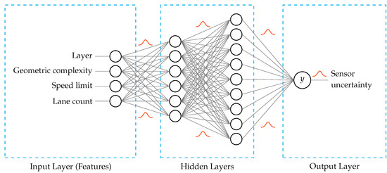
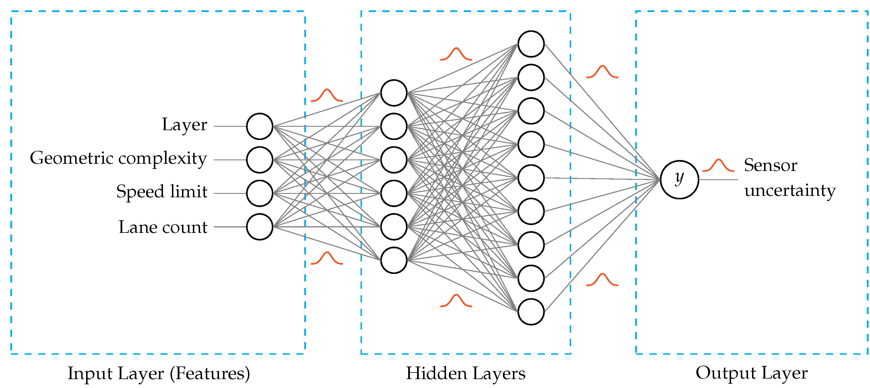
Incorporating a probabilistic approach into deep learning enables the elimination of uncertainty. To achieve the uncertainty elimination, such models assign lower confidence levels to inaccurate predictions. BNNs are utilized in this research to capture the epistemic uncertainty, which is the uncertainty related to the model fitness due to the availability of insufficient data from which to learn effectively. BNNs differ from standard neural networks in that BNNs learn probability distributions over the network weights to encode the uncertainty of the weights, whereas standard neural networks learn certain weight and bias values (see Figure 2). Before observing any data, a prior probability distribution is defined. Once data are observed, the model learns the parameters and transforms the distribution into a posterior distribution. In this work, the prior and posterior distributions are Gaussian in nature since the BNN output y is the expected sensor error indicating the amount of sensor uncertainty, which is a continuous variable. The features considered in the BNN model include road and environmental attributes such as the number of lanes and the weather conditions.

Ideally, high uncertainty in a BNN indicates samples that are far away from the evaluated data, while the uncertainty of close samples is low. Given a training dataset $\mathcal{D}=\left\{x^{\left(i\right)},y^{\left(i\right)}\right\}$, the optimal solution for estimating the posterior distribution of the network parameters is to use full Bayesian inference or Bayes’ theorem, expressed as

$$P\left(w\right|\mathcal{D})=\frac{P\left(\mathcal{D}\right|w\left)P\right(w)}{P\left(\mathcal{D}\right)},$$

(16)

where w denotes the network parameters; $P\left(w\right|\mathcal{D})$ and $P\left(w\right)$ are the posterior and prior parameter distributions, respectively; $P\left(\mathcal{D}\right|w)$ is the likelihood function; and $P\left(\mathcal{D}\right)$ is the probability of the training dataset occurring.

A prediction of a new sample, $P\left(y\right|x)$, can be computed by taking the expected value of the optimized posterior distribution, $P\left(w^{*}\right|\mathcal{D})$, as follows:

$$P\left(\widehat{y}\right|x)=E_{P\left(w^{*}\right|\mathcal{D})}P\left(\widehat{y}\right|x,w^{*}),$$

(17)

This expectation serves as the average prediction of an infinite number of neural networks, weighted by their posterior probabilities. Although this prediction is resistant to noise, an analytical solution for both the posterior distribution and the prediction is computationally intractable. Hence, we resort to approximation. In this work, a deterministic method, i.e., variational inference, is employed. The basic concept of the variational technique is to formulate the inference task as an optimization problem. This optimization problem is tackled by approximating the actual posterior distribution, $P\left(w\right|\mathcal{D})$, by an instance of tractable distributions, $Q\left(w\right|\theta )$; i.e., a $Q\left(w\right|\theta )$ that closely resembles $P\left(w\right|\mathcal{D})$ is determined. Because the variational posterior is Gaussian, it is parameterized by $\theta =\mu ,{\sigma }^2$ with a mean $\mu$ and a variance ${\sigma }^2$. Instead of querying $P\left(w\right|\mathcal{D})$, the BNN queries $Q\left(w\right|\theta )$ to obtain an approximate solution, which is formally accomplished by minimizing the Kullback–Leibler (KL) divergence between the two probability distributions $P\left(w\right|\mathcal{D})$ and $Q\left(w\right|\theta )$. The related optimization objective is called the variational free energy and is expressed as a combination of complexity and error losses:

$$F(\mathcal{D},\theta )=\underset{\mathrm{complexity}}{\underbrace{{\mathcal{D}}_{KL}\left(Q\left(w\right|\theta )\parallel P(w)\right)}}-\underset{\mathrm{error}}{\underbrace{\mathbb{E}{\left[logP\left(\mathcal{D}\right|w)\right]}_{Q\left(w\right|\theta )}}},$$

(18)

where the first term is the KL divergence between $Q\left(w\right|\theta )$ and $P\left(w\right)$, and the second term is the expectation of the likelihood function under the variational distribution $Q\left(w\right|\theta )$. The complexity cost determines the network cost, whereas the error cost determines the prediction accuracy

Rearranging the terms in Equation (18) allows the optimization objective function to be written as

$$F(\mathcal{D},\theta )=\mathbb{E}{\left[logQ\left(w\right|\theta )\right]}_{Q\left(w\right|\theta )}-\mathbb{E}{\left[logP\left(w\right)\right]}_{Q\left(w\right|\theta )}-\mathbb{E}{\left[logP\left(\mathcal{D}\right|w)\right]}_{Q\left(w\right|\theta )}.$$

(19)

Hence, samples $w^{\left(i\right)}$ drawn from $Q\left(w\right|\theta )$ can approximate the objective function as follows:

$$F(\mathcal{D},\theta )\approx \frac{1}{N}\sum _{i=1}^N\left[logQ(w^{\left(i\right)}|\theta )-logP(w^{\left(i\right)})-logQ(\mathcal{D}|w^{\left(i\right)})\right].$$

(20)

Each iteration of the training process involves a forward propagation phase and a backward propagation phase. In the forward propagation phase, a random sample is drawn from the variational distribution and propagated through the network until it reaches the final layer. Then, the approximate objective function (Equation (20)) can be evaluated. The first two terms of Equation (20) can be evaluated in each layer since they are independent of the data, while the third term can be evaluated only at the forward-propagation end due to its data dependence. In the backward propagation phase, the gradients of the parameters of the variational posterior distribution are computed, and their values are adjusted accordingly.

The BNN model produces different estimates for identical inputs during each run as new weights are sampled from the distributions each time to build the network and generate an output. As the model becomes more certain about its weights, the outputs produced for the same inputs reveal less variability. This epistemic uncertainty is reduced when AVs are exposed to increasingly many different scenarios. Moreover, the output of standard BNN models are a point estimate for a given input. In our proposed approach, the output is modeled as normal distribution with learnable parameters. In this case, the BNN model also incorporates the aleatoric uncertainty caused by irreducible noise in sensor data. Due to this merit, the model can be trained with the negative log-likelihood function as the loss function.

3.4. Pretraining Process

The predictive model starts with equal probabilities for the uncertainty in all road segments, resulting in equal predictions. To improve the initial results, our approach assumes that some data samples exist for pretraining purposes. In this stage, the BNN model is fed with estimates of sensor uncertainty as well as the associated road features and environmental conditions. The resultant model can be utilized as an initial pretrained model and refined as the approach continues to operate.

4. Evaluation and Discussion

Extensive experiments were conducted on a real dataset to evaluate the performance of the proposed approach. Python 3.9 was utilized for implementation. All experiments were carried out on a system running macOS 11.5 Big Sur with a 2.9 GHz dual-core Intel Core i5 processor and 8 GB of memory. The implementation of the Kalman filter was developed from scratch, whereas for the BNN implementation, Keras [49] and TensorFlow Probability [50] were used. We evaluated the uncertainty existing in the data and generated by the GNSS.

Our evaluation included two data sources. The first data source was the Ford AV dataset [51], which logs 18 trajectories captured by a fleet of Ford AVs under different environmental and driving conditions, including different weather, traffic, lighting, and construction conditions. With these diverse conditions, these data encompass different sources of uncertainty and thus are perfectly aligned with the objective of our proposed approach.

Table 1. Summary of the Ford AV dataset.

			Route Features
Acquisition Date	Vehicle	Log #	Freeway	Overpass	Tunnel	Cloudy	Sunny	Vegetation	Residential	Airport	University	Construction
4 August 2017	V2	1	✕	✕		✕
		2	✕		✕	✕				✕		✕
		3					✕		✕
		4					✕	✕			✕
		5		✕			✕	✕	✕
		6					✕	✕	✕			✕
	V3	1	✕	✕		✕
		2	✕		✕	✕				✕		✕
		3					✕		✕
		4					✕	✕			✕
		5		✕			✕	✕	✕
		6					✕	✕	✕			✕
26 October 2017	V2	1	✕	✕			✕					✕
		2	✕	✕	✕		✕			✕		✕
		3					✕		✕
		4					✕	✕			✕
		5		✕			✕	✕	✕
		6					✕	✕	✕			✕

summarizes the major features of the routes in the Ford AV dataset. The data were collected while the vehicles were being driven manually in Michigan.

The recorded coordinates were matched to the real-world road network in Open Street Map [52]. Accordingly, the attributes associated with the matched roads could be obtained and processed. To solve the map matching problem, a hidden Markov model approach was exploited [53]. Given the GNSS observations, each observation was matched to the most likely candidate road segment. An open-source routing software called Valhalla was utilized for map matching [54]. The GNSS traces were matched based on time, acceleration, and directional angles to achieve the best matching results.

Since our focus was on predicting GNSS uncertainty, we selected four features (layer, geometry, speed limit, lane count) that could capture degradation in GNSS performance and fed them into the predictive model. The layer feature indicates the existence of occlusions preventing signals from reaching the GNSS receiver. The layer feature could have a positive or negative number, where the former indicates bridges, and the latter indicates tunnels and under-bridge road segments; a layer value of zero indicates normal road segments. The geometric complexity feature indicates the number of points representing a particular road segment (also known as resolution). For instance, the geometric complexity feature for a simple straight road segment (a line) has only two points. The posted speed limit feature indicates the road type, such as a highway or a residential road. The lane count feature indicates the road width. On a large road segment, which typically may have multiple-lanes, there is a lower chance of signals being blocked by trees or buildings.

The architecture of the BNN consisted of four layers: an input layer, two hidden layers, and an output layer (see Figure 2). The input layer included four nodes representing the features mentioned earlier. The first and second hidden layers consisted of six and nine nodes, respectively. The output layer included only one node representing the sensor uncertainty. The sigmoid activation function was applied for each node in the BNN hidden layers. The optimizer utilized to train the model was the RMSprop algorithm. The BNN was designed to produce a normal distribution so that we could calculate how probable was it that the actual data would be seen in the model’s predicted distribution. Therefore, the model was trained with the negative log-likelihood as the loss function. We also evaluated the accuracy in terms of the root mean square error (RMSE) and the mean absolute error (MAE).

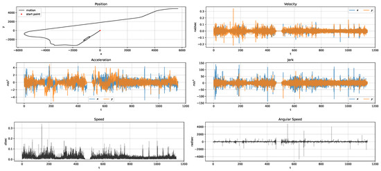
The EKF received sensory and derived measurements, including position, velocity, acceleration, jerk, speed, and angular speed. An instance of sensory measurements fed into the EKF is presented in Figure 3. Once the EKF had processed these measurements, the sensor uncertainty estimates were stored in the uncertainty pool. The stored estimates were aggregated by their associated road segments, and the average was computed. The resultant data consisted of 971 road segments for analysis. For evaluation purposes, we randomly selected 13 logs for training and 5 logs for testing. The selected test logs were Aug V2—Log 2, Aug V3—Log 1, Aug V3—Log 2, Aug V3—Log 6, and Oct V2—Log 3. The training set was shuffled and split into training and evaluation sets, corresponding to 82% and 18% of the samples, respectively. The entire approach was evaluated with earlier configurations on 13 out of the 18 logs. When testing the BNN outcomes, we predicted the GNSS uncertainties produced for the five different test logs and then compared those results with those estimated by the EKF. The findings revealed promising sensor uncertainty estimation performance.

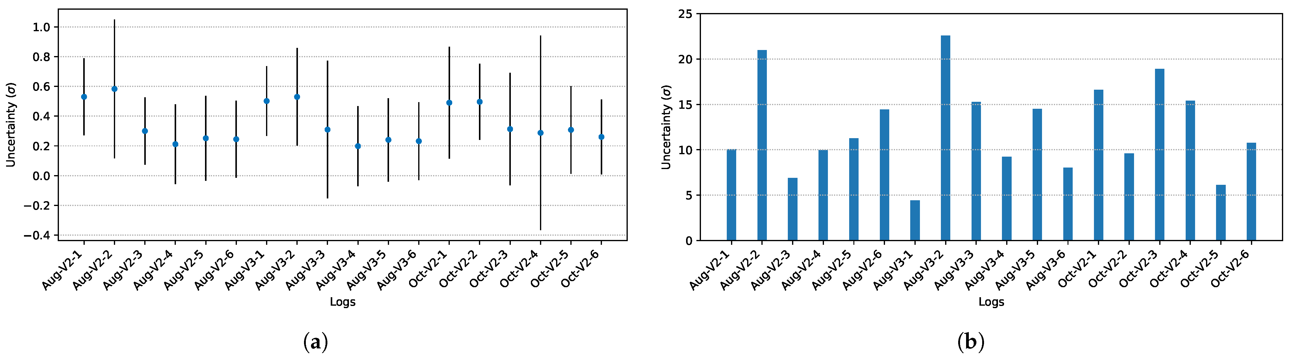
Figure 4a depicts considerable differences between the GNSS uncertainties on different routes. These discrepancies are anticipated due to varying environmental conditions. However, routes with the same features demonstrate similar trends. For instance, Vehicles 2 and 3 exhibit similar trends on their August routes. Nevertheless, at the micro level, these identical routes have different GNSS uncertainties on individual road segments. In other words, the uncertainties differ within the same road segments. Figure 4b illustrates the maximum GNSS uncertainties estimated for each route. It is apparent that in this case, the trends between Vehicles 2 and 3 disappear, and the differences between the maximum values can be large, such as the difference between the first logs in August for Vehicles 2 and 3, although they have identical route attributes but not environmental attributes. The fact that these vehicles run under different conditions is confirmed by examining the standard deviations of the GNSS uncertainties for the associated routes in Figure 4a.

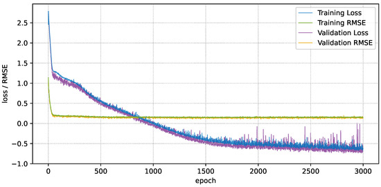
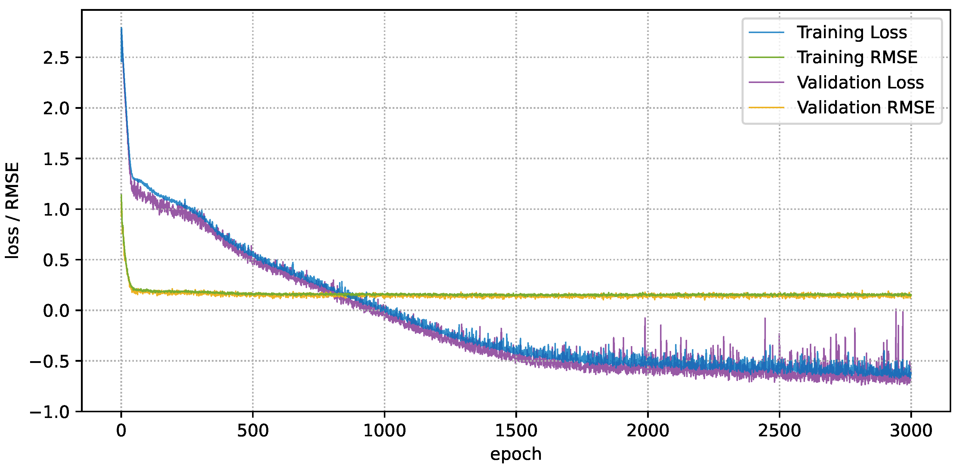
Figure 5 shows how the negative log-likelihood loss changes over the epochs along with the RMSE values for both the training and evaluation datasets. As can be observed, the learning curve converges very quickly during training, after approximately 1800 epochs, while the validation set average loss exhibits fluctuations across the finally epochs. Since the proposed approach is designed to handle thousands of samples, this rapid convergence could be related to the relatively low number of samples used for training. Nevertheless, the difference between the prediction accuracies on the training and evaluation sets is not significant, with training RMSE = 0.15 and evaluation RMSE = 0.155. Moreover, the training losses are higher during some epochs because relatively few samples were used for validation. An evaluation of the trained model on unseen data demonstrates an accuracy very close to the training accuracy (i.e., RMSE = 0.157), which implies that the model is not overfitted.

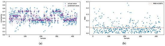
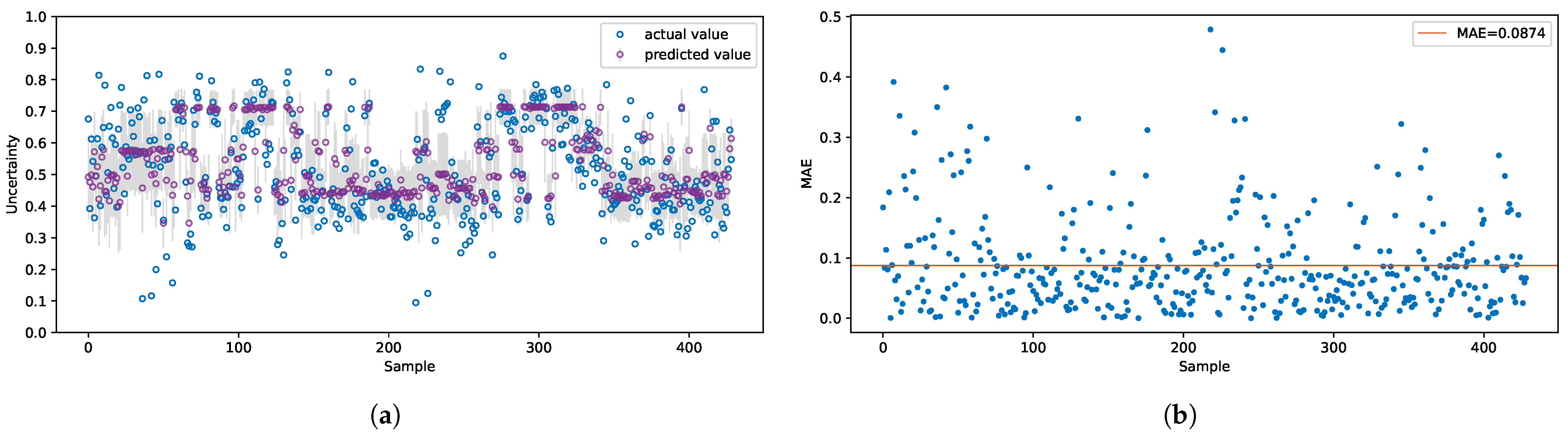
Each time being called the model produces different outputs because the weights are sampled from the given distributions. Figure 6a shows an instance of BNN prediction results for the test datasets. The grey vertical bars depict the 95% confidence intervals of the associated predictions. The less certain the model predictions are, the wider the intervals are seen in the output. It can be seen in Figure 6a that very few points are not predicted accurately. We ascribe mispredictions to the lack of similar examples in the training dataset. For these particular predictions, the RMSE and MAE are 0.119 and 0.087, respectively, (Figure 6b). It is apparent from Figure 6b that most of GNSS uncertainties are predicted with errors of less than 0.1 meters.

If provided with a model with a high level of confidence in its estimates of sensor uncertainty, the decision-making and planning for AVs could potentially be improved. Armed with the knowledge of the uncertainty of each sensor on every road segment, an AV could avoid or better maneuver through road segments with high uncertainty. Moreover, the AV might be able to set sensor preferences or prioritize road segments based on their high associated sensing accuracy. In this way, better decisions regarding challenging situations could certainly lead to safer navigation.

5. Conclusions and Future Research

This paper presents an end-to-end approach for exploiting the EKF and a BNN model with contextual information to predict the sensor uncertainties arising in challenging situations. The approach incorporates the EKF to measure the error encountered in the current situation. Using this error, the sensor uncertainty is estimated and associated with the context or environmental information for use in predicting future uncertainties. The proposed approach considers epistemic uncertainties, which are related to the lack of knowledge, and aleatoric uncertainties, which are related to stochastic nature of the data acquisition process. The results show that our learning approach performs very well in predicting GNSS uncertainties in real data. This approach has the potential to improve navigation safety for passengers and road users. With advance knowledge of possible sensor failures, AVs can better maneuver through challenging road segments that present risky conditions. Applications of our proposed approach are not limited to path planning; rather, all AV modules, such as localization, lane-keeping assistance, blind-spot detection, and object detection, can benefit from sensor uncertainty estimates. For instance, upon determination that a navigation-related sensor provides estimates with high uncertainty, the localization module can disregard its readings, avoiding localization with large errors.

However, given that neural networks are data intensive, through sharing data among AVs, the proposed approach can alleviate possible uncertain situations. Since sensors are fabricated by varying vendors and have different configurations, future research should consider modeling features of sensor configurations and qualities along with the environmental features. Moreover, a new decision-making module should be developed to analyze the sensor uncertainty estimates and support AVs in making the proper decision for each task.

References

- Panzieri, S.; Pascucci, F.; Ulivi, G. An outdoor navigation system using GPS and inertial platform. IEEE/ASME Trans. Mechatron. 2002, 7, 134–142. [Google Scholar] [CrossRef]
- Kaelbling, L.P.; Littman, M.L.; Cassandra, A.R. Planning and acting in partially observable stochastic domains. Artif. Intell. 1998, 101, 99–134. [Google Scholar] [CrossRef] [Green Version]
- Platt, R.; Tedrake, R.; Kaelbling, L.; Lozano-Pérez, T. Belief space planning assuming maximum likelihood observations. In Proceedings of the 6th Robotics: Science and Systems Conference, Zaragoza, Spain, 27–30 June 2010. [Google Scholar] [CrossRef]
- Urmson, C.; Anhalt, J.; Bagnell, D.; Baker, C.; Bittner, R.; Clark, M.N.; Dolan, J.; Duggins, D.; Galatali, T.; Geyer, C.; et al. Autonomous driving in urban environments: Boss and the Urban Challenge. J. Field Robot. 2008, 25, 425–466. [Google Scholar] [CrossRef] [Green Version]
- Zhang, J.; Singh, S. Visual-lidar odometry and mapping: Low-drift, robust, and fast. In Proceedings of the 2015 IEEE International Conference on Robotics and Automation (ICRA), Seattle, WA, USA, 26–30 May 2015; pp. 2174–2181. [Google Scholar] [CrossRef]
- Yan, M.; Wang, J.; Li, J.; Zhang, C. Loose coupling visual-lidar odometry by combining VISO2 and LOAM. In Proceedings of the 2017 36th Chinese Control Conference (CCC), Dalian, China, 26–28 July 2017; pp. 6841–6846. [Google Scholar] [CrossRef]
- Xiang, Z.; Yu, J.; Li, J.; Su, J. ViLiVO: Virtual LiDAR-Visual Odometry for an Autonomous Vehicle with a Multi-Camera System. In Proceedings of the 2019 IEEE/RSJ International Conference on Intelligent Robots and Systems (IROS), Macau, China, 3–8 November 2019; pp. 2486–2492. [Google Scholar] [CrossRef] [Green Version]
- Yang, Y.; Tang, D.; Wang, D.; Song, W.; Wang, J.; Fu, M. Multi-camera visual SLAM for off-road navigation. Robot. Auton. Syst. 2020, 128, 103505. [Google Scholar] [CrossRef]
- Wahyudi; Listiyana, M.S.; Sudjadi; Ngatelan. Tracking Object based on GPS and IMU Sensor. In Proceedings of the 2018 5th International Conference on Information Technology, Computer, and Electrical Engineering (ICITACEE), Semarang, Indonesia, 27–28 September 2018. [Google Scholar] [CrossRef]
- Melotti, G.; Premebida, C.; Gonçalves, N. Multimodal Deep-Learning for Object Recognition Combining Camera and LIDAR Data. In Proceedings of the 2020 IEEE International Conference on Autonomous Robot Systems and Competitions (ICARSC), Ponta Delgada, Portugal, 15–17 April 2020; pp. 177–182. [Google Scholar] [CrossRef]
- Nobis, F.; Geisslinger, M.; Weber, M.; Betz, J.; Lienkamp, M. A Deep Learning-based Radar and Camera Sensor Fusion Architecture for Object Detection. In Proceedings of the 2019 Sensor Data Fusion: Trends, Solutions, Applications (SDF), Bonn, Germany, 15–17 October 2019; pp. 1–7. [Google Scholar] [CrossRef]
- Li, Z.; Yan, M.; Jiang, W.; Xu, P. Vehicle Object Detection Based on RGB-Camera and Radar Sensor Fusion. In Proceedings of the 2019 International Joint Conference on Information, Media and Engineering (IJCIME), Osaka, Japan, 17–19 December 2019; pp. 164–169. [Google Scholar] [CrossRef]
- Asvadi, A.; Girão, P.; Peixoto, P.; Nunes, U. 3D object tracking using RGB and LIDAR data. In Proceedings of the 2016 IEEE 19th International Conference on Intelligent Transportation Systems (ITSC), Rio de Janeiro, Brazil, 1–4 November 2016; pp. 1255–1260. [Google Scholar] [CrossRef]
- Pfeuffer, A.; Dietmayer, K. Optimal Sensor Data Fusion Architecture for Object Detection in Adverse Weather Conditions. In Proceedings of the 2018 21st International Conference on Information Fusion (FUSION), Cambridge, UK, 10–13 July 2018; pp. 1–8. [Google Scholar] [CrossRef] [Green Version]
- Pfeuffer, A.; Dietmayer, K. Robust semantic segmentation in adverse weather conditions by means of sensor data fusion. In Proceedings of the 2019 22th International Conference on Information Fusion (FUSION), Ottawa, ON, Canada, 2–5 July 2019; pp. 1–8. [Google Scholar]
- Porav, H.; Bruls, T.; Newman, P. I Can See Clearly Now: Image Restoration via De-Raining. In Proceedings of the 2019 International Conference on Robotics and Automation (ICRA), Montreal, QC, Canada, 20–24 May 2019; pp. 7087–7093. [Google Scholar] [CrossRef] [Green Version]
- Sakaridis, C.; Dai, D.; Van Gool, L. Semantic Foggy Scene Understanding with Synthetic Data. Int. J. Comput. Vis. 2018, 126, 973–992. [Google Scholar] [CrossRef] [Green Version]
- Piewak, F.; Pinggera, P.; Schafer, M.; Peter, D.; Schwarz, B.; Schneider, N.; Enzweiler, M.; Pfeiffer, D.; Zollner, M. Boosting LiDAR-based Semantic Labeling by Cross-Modal Training Data Generation. In Proceedings of the European Conference on Computer Vision (ECCV) Workshops, Munich, Germany, 8–14 September 2018. [Google Scholar]
- Park, S.J.; Hong, K.S.; Lee, S. RDFNet: RGB-D Multi-Level Residual Feature Fusion for Indoor Semantic Segmentation. In Proceedings of the IEEE International Conference on Computer Vision (ICCV), Venice, Italy, 22–29 October 2017. [Google Scholar]
- Hazirbas, C.; Ma, L.; Domokos, C.; Cremers, D. FuseNet: Incorporating Depth into Semantic Segmentation via Fusion-Based CNN Architecture. In Computer Vision—ACCV 2016; Lai, S.H., Lepetit, V., Nishino, K., Sato, Y., Eds.; Springer International Publishing: Cham, Switzerland, 2017; pp. 213–228. [Google Scholar]
- Caltagirone, L.; Scheidegger, S.; Svensson, L.; Wahde, M. Fast LIDAR-based road detection using fully convolutional neural networks. In Proceedings of the 2017 IEEE Intelligent Vehicles Symposium (IV), Los Angeles, CA, USA, 11–14 June 2017; pp. 1019–1024. [Google Scholar] [CrossRef] [Green Version]
- Fu, C.; Sarabakha, A.; Kayacan, E.; Wagner, C.; John, R.; Garibaldi, J.M. Input uncertainty sensitivity enhanced nonsingleton fuzzy logic controllers for long-term navigation of quadrotor UAVs. IEEE/ASME Trans. Mechatron. 2018, 23, 725–734. [Google Scholar] [CrossRef]
- Foresti, G.L.; Regazzoni, C.S. Multisensor data fusion for autonomous vehicle navigation in risky environments. IEEE Trans. Veh. Technol. 2002, 51, 1165–1185. [Google Scholar] [CrossRef]
- Hossein, T.N.N.; Mita, S.; Long, H. Multi-sensor data fusion for autonomous vehicle navigation through adaptive particle filter. In Proceedings of the 2010 IEEE Intelligent Vehicles Symposium, La Jolla, CA, USA, 21–24 June 2010; pp. 752–759. [Google Scholar] [CrossRef]
- Smallwood, R.D.; Sondik, E.J. The optimal control of partially observable Markov processes over a finite horizon. Oper. Res. 1973, 21, 1071–1088. [Google Scholar] [CrossRef]
- Sondik, E.J. The optimal control of partially observable Markov processes over the infinite horizon: Discounted costs. Oper. Res. 1978, 26, 282–304. [Google Scholar] [CrossRef]
- Kavraki, L.E.; Švestka, P.; Latombe, J.C.; Overmars, M.H. Probabilistic roadmaps for path planning in high-dimensional configuration spaces. IEEE Trans. Robot. Autom. 1996, 12, 566–580. [Google Scholar] [CrossRef] [Green Version]
- LaValle, S.M.; Kuffner, J.J. Randomized kinodynamic planning. Int. J. Robot. Res. 2001, 20, 378–400. [Google Scholar] [CrossRef]
- Prentice, S.; Roy, N. The belief roadmap: Efficient planning in belief space by factoring the covariance. Int. J. Robot. Res. 2009, 28, 1448–1465. [Google Scholar] [CrossRef]
- Stilman, M.; Schamburek, J.U.; Kuffner, J.; Asfour, T. Manipulation Planning Among Movable Obstacles. In Proceedings of the 2007 IEEE International Conference on Robotics and Automation, Rome, Italy, 10–14 April 2007; pp. 3327–3332. [Google Scholar] [CrossRef]
- Berenson, D.; Kuffner, J.; Choset, H. An optimization approach to planning for mobile manipulation. In Proceedings of the 2008 IEEE International Conference on Robotics and Automation, Pasadena, CA, USA, 19–23 May 2008; pp. 1187–1192. [Google Scholar] [CrossRef]
- Yershova, A.; LaValle, S.M. Improving Motion-Planning Algorithms by Efficient Nearest-Neighbor Searching. IEEE Trans. Robot. 2007, 23, 151–157. [Google Scholar] [CrossRef]
- Koyuncu, E.; Ure, N.K.; Inalhan, G. Integration of Path/Maneuver Planning in Complex Environments for Agile Maneuvering UCAVs. J. Intell. Robot. Syst. 2009, 57, 143. [Google Scholar] [CrossRef]
- Luders, B.D.; Karaman, S.; Frazzoli, E.; How, J.P. Bounds on tracking error using closed-loop rapidly-exploring random trees. In Proceedings of the 2010 American Control Conference, Baltimore, MD, USA, 30 June–2 July 2010; pp. 5406–5412. [Google Scholar] [CrossRef]
- Tedrake, R.; Manchester, I.R.; Tobenkin, M.; Roberts, J.W. LQR-trees: Feedback Motion Planning via Sums-of-Squares Verification. Int. J. Robot. Res. 2010, 29, 1038–1052. [Google Scholar] [CrossRef] [Green Version]
- Van Den Berg, J.; Abbeel, P.; Goldberg, K. LQG-MP: Optimized path planning for robots with motion uncertainty and imperfect state information. Int. J. Robot. Res. 2011, 30, 895–913. [Google Scholar] [CrossRef]
- Bry, A.; Roy, N. Rapidly-exploring random belief trees for motion planning under uncertainty. In Proceedings of the 2011 IEEE International Conference on Robotics and Automation, Shanghai, China, 9–13 May 2011; pp. 723–730. [Google Scholar]
- Van Den Berg, J.; Patil, S.; Alterovitz, R. Motion planning under uncertainty using iterative local optimization in belief space. Int. J. Robot. Res. 2012, 31, 1263–1278. [Google Scholar] [CrossRef]
- Sun, W.; van den Berg, J.; Alterovitz, R. Stochastic extended LQR for optimization-based motion planning under uncertainty. IEEE Trans. Autom. Sci. Eng. 2016, 13, 437–447. [Google Scholar] [CrossRef] [Green Version]
- Alharbi, M.; Karimi, H.A. A global path planner for safe navigation of autonomous vehicles in uncertain environments. Sensors 2020, 20, 6103. [Google Scholar] [CrossRef] [PubMed]
- Kiureghian, A.D.; Ditlevsen, O. Aleatory or epistemic? Does it matter? Struct. Saf. 2009, 31, 105–112. [Google Scholar] [CrossRef]
- Neal, R.M. Bayesian Learning for Neural Networks; Springer Science & Business Media: New York, NY, USA, 2012; ISBN 978-1-4612-0745-0. [Google Scholar]
- MacKay, D.J.C. A Practical Bayesian Framework for Backpropagation Networks. Neural Comput. 1992, 4, 448–472. [Google Scholar] [CrossRef]
- Bishop, C.M. Bayesian Neural Networks. J. Braz. Comput. Soc. 1997, 4, 61–68. [Google Scholar] [CrossRef]
- Blei, D.M.; Kucukelbir, A.; McAuliffe, J.D. Variational Inference: A Review for Statisticians. J. Am. Stat. Assoc. 2017, 112, 859–877. [Google Scholar] [CrossRef] [Green Version]
- Graves, A. Practical variational inference for neural networks. In Proceedings of the 25th Annual Conference on Neural Information Processing Systems, Granada, Spain, 12–17 December 2011; pp. 2348–2356. [Google Scholar]
- Chang, G. Robust Kalman filtering based on Mahalanobis distance as outlier judging criterion. J. Geod. 2014, 88, 391–401. [Google Scholar] [CrossRef]
- Chang, G.; Liu, M. An adaptive fading Kalman filter based on Mahalanobis distance. Proc. Inst. Mech. Eng. Part G J. Aerosp. Eng. 2015, 229, 1114–1123. [Google Scholar] [CrossRef]
- Chollet, F. Keras. Available online: https://keras.io (accessed on 20 June 2021).
- Dillon, J.V.; Langmore, I.; Tran, D.; Brevdo, E.; Vasudevan, S.; Moore, D.; Patton, B.; Alemi, A.; Hoffman, M.; Saurous, R.A. TensorFlow Distributions. arXiv 2017, arXiv:cs.LG/1711.10604. [Google Scholar]
- Agarwal, S.; Vora, A.; Pandey, G.; Williams, W.; Kourous, H.; McBride, J. Ford Multi-AV Seasonal Dataset. Int. J. Robot. Res. 2020, 39, 1367–1376. [Google Scholar] [CrossRef]
- OpenStreetMap Contributors. Planet Dump. Available online: https://www.openstreetmap.org (accessed on 18 June 2021).
- Newson, P.; Krumm, J. Hidden Markov Map Matching Through Noise and Sparseness. In Proceedings of the 17th ACM SIGSPATIAL International Conference on Advances in Geographic Information Systems (ACM SIGSPATIAL GIS 2009), Seattle, WA, USA, 4–6 November 2009; pp. 336–343. [Google Scholar]
- Valhalla Contributors. Valhalla: Open Source Routing Engine for OpenStreetMap. Available online: https://valhalla.readthedocs.io (accessed on 18 June 2021).
Publisher’s Note: MDPI stays neutral with regard to jurisdictional claims in published maps and institutional affiliations. |
© 2021 by the authors. Licensee MDPI, Basel, Switzerland. This article is an open access article distributed under the terms and conditions of the Creative Commons Attribution (CC BY) license (https://creativecommons.org/licenses/by/4.0/).