Physics-Based and Data-Enhanced Model for Electric Drive Sizing during System Design of Electrified Powertrains

Abstract

In multi-drive electrified powertrains, the control strategy strongly influences the component load collectives. Due to this interdependency, the component sizing becomes a difficult task. This paper comprehensively analyses different electric drive system sizing methods for multi-drive systems in the literature. Based on this analysis, a new data-enhanced sizing approach is proposed. While the characteristic is depicted with a physics-based polynomial model, a data-enhanced limiting function ensures the parameter variation stays within a physically feasible range. Its beneficial value is demonstrated by applying the new model to a powertrain system optimization. The new approach enables a detailed investigation of the correlations between the characteristic of electric drive systems and the overall vehicle energy consumption for varying topologies. The application results demonstrate the accuracy and benefit of the proposed model.

1. Introduction

A growing environmental awareness and increasingly stringent $C{O}_2$ limitations in worldwide markets have resulted in an accelerated electrification of modern passenger vehicles. In recent years, most car manufacturers have developed or announced new all-electric platforms. In addition to battery electric vehicles (BEV), the hybridization of conventional powertrains is also an important factor in order to meet the consumption reduction targets. Hybridized powertrains are about to supersede conventional powertrains within the next years [1,2].

Hybrid electric vehicles (HEV) range from 48 V-Systems with 15–30 kW of electric system power to plug-in HEVs with 60–100 kW of electric system power able to traverse up to a 100 km range in all-electric mode.

In contrast to conventional powertrains, all HEV- and several BEV-powertrains consist of more than one drive unit. As a result, the torque and speed requirements of each drive unit are no longer solely dependent on the driving task but are influenced by the operating strategy. This fact makes the sizing procedure of the electric traction motors more complicated [3,4], and it should be carried out on the system-level [5]. The resulting combined plant and controller optimization problem necessitates computationally efficient yet accurate models for the electric drive system (EDS) [6]. Such models should also allow a continuous variation of all important parameters.

In the recent literature, many authors have focused on the system-level EDS design. However, in most cases, the EDS models are too simple, especially for efficiency. In contrast to industry machines, the EDS design is no longer an optimization of the rated point. For traction machines, the system efficiency highly depends on the shape and location of the EDS efficiency characteristic [7]. Many papers only focus on a variation of the main EDS parameters, such as power or torque. Only a few publications consider a variation of the efficiency characteristic shape [8,9,10].

The utilized methods can be classified into two categories depending on the level the parameter variation is conducted on: (1) a variation on the component level and (2) a variation on the system level. An illustration is given in Figure 1. If the parameters on the component level are varied (e.g., geometry, winding, material), the parameters on the system level (e.g., torque, power, efficiency) are the output of the EDS model. A high number of variation parameters is necessary to cover the entire valid design space. Since such a large number of variation parameters is computationally inefficient, parts of the valid design space will be ignored. If, in contrast, the parameters are directly varied on the system level, only a few variation parameters are necessary to cover the valid design space. A variation on the system level, however, imposes a risk of permitting an investigation outside of the valid design space. In some cases, parts of the valid design space may be ignored due to simplifications in the utilized models. For a better distinction, parameters on the component level are denoted as design variables, whereas parameters on the system level are simply identified as parameters.

This paper proposes a new data-enhanced EDS model. The model is able to continuously vary all relevant parameters directly on the system level (e.g., torque, power, maximum speed, efficiency characteristic) while limiting the variation parameters to the valid design space. The electro-mechanical performance of the permanent magnet synchronous machine and the inverter is modelled using a physics-based polynomial model. Based on a database of FE-calculated designs, a limiting function to restrict the variation range is conceived. The great advantage of the new approach is that once this limiting function is constructed, no further detailed knowledge on electric machines is necessary to investigate the influences of the EDS design on global optimization targets, such as the energy consumption of multi-drive systems.

Section 2 reviews different methods used to model electric drive systems during powertrain system design. The methods are classified depending on the variation parameters, and the advantages and disadvantages are discussed. In Section 3, the new data-enhanced model is presented before it is applied to a powertrain system optimization in Section 4. The results in Section 5 demonstrate the accuracy and robustness of the EDS model and illustrate its beneficial value at the system-level design phase.

2. Methods for Modelling Electric Drive Systems

Nicoletti et al. [11] performed a literature review on the design parameters necessary for the high-level powertrain definition for an electric vehicle. In the case of the electric machine sizing, the authors found six parameters as particularly relevant: rotational speed, machine torque and power, gear ratio, geometric dimensions, and weight. Li et al. [7] emphasize the importance of EDS efficiency as an additional parameter which is often neglected, especially in multi-machine systems.

Given the design parameters, several methods are possible for determining the optimal values. This process is often referred to as component sizing. Huang et al. [12] distinguish between traditional sizing methods and optimization-based component sizing. The traditional sizing methods are often based on experience or databases and usually are not able to find the optimal solution. In the recent literature, the optimization-based methods usually couple the component sizing problem with the operating strategy optimization, thus becoming a combined optimization problem. The operating strategy manages the power-flow between the different traction components (i.e., engine and electric machine) with the aim to minimize the overall energy consumption. In [12], the optimization-based component sizing is further divided into sequential, iterative, nested, and simultaneous optimization procedures.

The sequential approach is the state-of-the-art method for detailed investigations on the component level. Thereby, an optimization incorporating FE analysis of the electric machine is often performed [13]. For example, [14,15,16,17] undertake a detailed optimization of the electric machine, where the electric machine’s cycle efficiency is one objective. However, if more than one drive unit is installed, the operating points of each drive component depend highly on the specific optimal operating strategy and are no more directly dependent on the driving cycle. The EDS operating points are a priori unknown. Hence, for powertrains with more than one drive unit (e.g., HEV), the sequential approach is inappropriate for component sizing on the system level.

A simultaneous optimization leads to a more complex mathematical problem formulation with a very large number of variables in the problem (easily tens of thousands [18]) and is only possible if the model is heavily simplified. Pourabdollah et al. [18] introduced a novel method to simultaneously optimize the size of powertrain components and the operating strategy in a plug-in HEV. The authors apply a convex programming-based operating strategy, and the components are modelled with quadratic loss functions. A similar approach is used by Hu et al. [3] to simultaneously optimize the components and the operating strategy layer for a BEV with simultaneous front and rear axle drives.

In a nested approach, all layers are optimized top down. During each iteration in one layer, all sub-layers are optimized. In the case of nested sizing and control schemes, the component sizing is optimized in an outer loop, whereas the control optimization is conducted in an inner loop. The nested optimization method leads to a higher number of total function evaluations but is able to find the global optimum [12,19]. A comparison of different nested optimization procedure frameworks is given in [5,20]. In contrast to the simultaneous approach, ordinary component models can be used for a nested optimization method. Due to the higher number of total function evaluations, however, simplifications are helpful to reduce the computational effort.

To perform the optimization, the parameters have to be varied. A parameter variation can be conducted either discretely, e.g., by varying loss maps stored in a database [21], or continuously, e.g., by scaling a base machine using scaling laws [22]. Whereas a discrete parameter variation imposes additional requirements on the optimization algorithm, a continuous parameter variation simplifies the optimization process and ensures that the global optimum will be determined.

Several methods for generating EDS models with varying parameters exist.

Table 1. Classification of EDS modelling methods for component sizing found in literature.

Parameter Variation	Method	Literature
Component level	Analytical calculation	[7,23,24,25,26]
	Equivalent circuit models	[27,28]
	Scaling laws	[6,22,29,30,31,32]
	Neuronal networks	[13,33]
System level	Deforming loss maps	[19,20,34,35,36,37,38,39]
	Classified database	[9,10]
	Mathematical models	[3,4,8,40,41]

gives a summary of different methods found in the literature. The methods can be divided into two categories depending on the level on which the parameters are varied. Those two categories along with the related methods will be described in the following.

2.1. Component Level

A parameter variation on the component level varies the component design variables. Such design variables can be geometry parameters such as machine diameter and length, winding parameters such as number of turns or slots per pole per phase, electric parameters such as current and voltage, or material parameters such as magnet force and grade. This approach leads to a higher modelling depth of the investigated component. A deep knowledge of each specific component is necessary, leading to a multidisciplinary character of the problem. These methods include a large number of possible design parameters to be varied. The effect of a variation on the characteristic output of the component, and therefore the input to the inner optimization loop, is unknown. Such methods inherently allow conclusions identifying the influence of a parameter variation on the resulting installation space, weight, inertia, and cost.

By using analytical calculation methods, the entire EDS design process including stator and rotor design, winding design, and material selection is conducted at each function evaluation. The used models highly depend on the considered machine type and topology. Analytical calculations are considered as computationally efficient. To take into account the nonlinear properties of the materials, however, several iterations are necessary to obtain a valid saturation state. In addition, the calculation of loss maps during post-processing requires an additional optimization procedure. Furthermore, the achievable accuracy is limited, especially for the core losses of highly utilized synchronous machines with embedded magnets. Kalt et al. [42] published an electric machine design tool for the automated design and calculation of efficiency maps based on an analytical calculation using few input parameters. This model was applied in [24] to investigate the influence of the design parameters on the cycle efficiency. A similar tool is used in [25]. In order to simplify and accelerate the process, LeBerr et al. [25] neglect the saturation effects. Li et al. [7] proposed a method to directly derive loss maps of an induction machine based on design parameters, avoiding the aforementioned additional optimization during post-processing.

Another method can be the usage of equivalent circuit modelling. The electric machine’s characteristic is then described by a few parameters of a linear network such as resistances and inductance. Such models are able to predict the performance and loss characteristics at any specific operating point. They are, however, dependent on the considered machine type. After having estimated the parameters of the linear network by FE simulation, they can be varied in order to investigate different machines. Grunditz [27] adapted the parameters for a change in the machine’s active length. A difficulty, however, consists in the dependence of those parameters on the phase current and current advance angle due to magnetic saturation in the steel material. Eroglu et al. [28] neglect the effect of saturation by considering the inductance to be constant.

The most commonly used method to vary parameters on the component level are so-called scaling laws of electric machines. They take advantage of the separation of the FE-based calculation process into the parts FE analysis and post-processing. After solving Maxwell’s equations, the nonlinear relation between current (magnetomotive force) and magnetic flux is known. Without further increasing the maximum magnetomotive force, the machine’s length and the number of turns in the winding can be varied before calculating the characteristic loss map in the post-processing. Even a variation of the machine’s outer diameter is possible if all dimensions in the cross-sectional area are scaled by the same factor. A very high accuracy of the results over a broad variation range is achieved. This method was described by Stipetic et al. [29] for permanent magnet synchronous machines and was extended to induction machines by Nell et al. [31].

The former restriction, to be able to only vary the three parameters of length, diameter, and number of turns, can be improved by using artificial neuronal networks (ANN). This method includes the training of an ANN to a previously calculated database. The input of the model can be any machine parameter, whereas the output is a loss map. This approach was demonstrated by Gletter et al. [33], where the model was trained for the input parameters length, diameter, and number of turns. Zăvoianu et al. [13] trained their model to predict several scalar optimization objectives such as efficiency and cogging torque in a specific operating point instead of the prediction of entire loss maps.

2.2. System Level

Using a parameter variation on system level, the output of the component model is varied. The varied parameters become, for example, maximum torque, rated speed, maximum speed, or efficiency. Such a variation on the system level reduces the necessary modelling depth in the components. The computational effort is reduced, and a more flexible and easy-to-understand component model is possible. These models allow the system developer to investigate component variations without having deeper knowledge of the component itself. This is why such modelling methods are widespread in the literature (cf. Table 1). However, models in this second category usually incorporate assumptions and simplifications, leading to a reduced accuracy. In addition, it is difficult to find an inference back to the component design variables. This makes it hard to restrict the parameter range to a valid area. As a result, such methods can very well describe the influence of a variation in the component’s characteristics on the system output, but it may be that the investigated component is physically not feasible (cf. Figure 1).

If the variation of the parameters is conducted on system level, the most common method is the deformation of a predefined loss map, as used in [19,20,35,37,38,39]. This base characteristic can be the result of a preliminary calculation or a measurement. By varying the machine’s maximum torque and nominal speed, the loss map is stretched and compressed. Such a variation is similar to the variation of the machine’s length and number of turns when using the scaling laws previously described, even though much faster. Several simplifications are met to scale the EDS by deforming the loss map [19]. These simplifications lead to a restricted applicable variation range, and the influence of such a variation on the power electronics losses cannot be considered. Another disadvantage of this method is the lack of varying the efficiency characteristic in terms of shifting the efficiency optimum to other regions.

If a variation method based on databases is used, a variation of the efficiency characteristic is also possible. The database in these methods consists of several tens or hundreds of FE-calculated or measured loss maps which are classified by characteristic parameters. Domingues et al. [9] classifies 20 designs in categories according to their outer diameter and constant power speed range. The 20 designs can further be scaled in machine length to achieve the torque and power requirements. The presented approach allows for the investigation of different efficiency characteristics. A variation between different characteristics occurs in discrete steps. Vaillant [10] avoids this problem by interpolating between the stored characteristic loss maps to generate a new characteristic. However, there is no guarantee that the outcome is feasible in a physical sense, which is a major drawback of such an interpolation.

In contrast to the physics-based models described before, some studies use mathematical models to depict and vary loss maps of electric drive systems. Hellberg et al. [8] use elliptic paraboloids to model the efficiency map of electric machines. In the first step, the model is fitted to a measured efficiency using a least-min-square optimization. To generate new characteristic maps, additional parameters for shifting and rotating the paraboloid are introduced. A radial green function was used by Boehme et al. [41] to find a smooth power loss representation, which is later scaled linearly only in the torque direction. The scaling approach used ignores a variation of the efficiency characteristic. In convex programming optimization frames, typically the electric machine’s losses are modelled with a second order polynomial and are scaled linearly with torque [3,4]. Again, the variation of the efficiency characteristic is ignored for the sake of obtaining strongly simplified component models. In conclusion, those mathematical models are easy to implement, fast to evaluate, and allow a continuous exploration of the entire design space—including a variation of the efficiency characteristic—if applied correctly. However, they show limited accuracy and have no or little physical context.

To avoid the latter problem, a polynomial model for the losses in electric machines based on physical considerations is proposed in [43]. As the model is mainly intended for machines in industry applications, it is only valid in the base-speed region in motoring mode. Decker et al. [40] recently proposed a similar physics-based polynomial model which is extended to the field-weakening region and the generating mode and is capable of modelling all major EDS losses (i.e., electric machine and inverter). This model is also able to predict the DC-bus voltage dependency of the losses and therefore is applicable to automobile applications.

None of the above discussed methods allows a computationally efficient systematic variation of the entire EDS characteristics while ensuring an application-specific feasible design. Only the loss model in [40] allows a systematic variation of the loss map, but further extensions are necessary to model the limiting curves and to ensure that the modelled EDS is feasible.

3. Data-Enhanced Electric Drive System Model

In the previous section, different methods found in the literature to model and vary the characteristics of EDS within a system optimization process were summarized and discussed. Two levels for parameter variations have been introduced. This study proposes a new data-enhanced EDS model to vary parameters on the system level by combining the advantages of mathematical models and database-oriented approaches (cf. Table 1). This work models the EDS loss maps using the physics-based polynomial model developed in [40] and extends the model to predict the maximum torque curves. The proposed approach allows a continuous variation of the EDS characteristics. To ensure that the variation only takes place within a feasible range, a limiting function is employed. This limiting function consists of a random forest algorithm which is trained to a database of prior FE-calculated EDS. Prior to the training process, the database can be filtered for freely selectable design variables such as installation space, inverter phase current, or usable materials. The limiting function will then restrict the parameter range used for the EDS model. Once the limiting function is implemented, the proposed method allows the inclusion of the EDS model into a powertrain system optimization procedure. One possible objective would be to maximize the consumption savings while minimizing the electric system power. The overall process is presented in Figure 2.

The contributions of this work are twofold. First, the existing methods in the literature to describe and vary the EDS characteristics’ behaviour are summarized and compared. The results have been given in the previous section. Second, this work proposes a new data-enhanced model allowing a continuous variation of the EDS characteristics restricted to freely selectable physical boundaries such as installation space, inverter phase current, or usable materials. The new approach allows a detailed investigation of the correlation between EDS characteristics and overall vehicle efficiency for different topologies and driving environments. The polynomial model is limited to permanent magnet synchronous machines (PMSM), though an adaption to other machine types may be possible.

3.1. Polynomial Model

The polynomial model consists of two individual sub-models completely characterizing the EDS under test. The two sub-models are a loss model describing the occurring losses at a specific operating point and a maximum torque model describing the maximum torque ability of the EDS for a given speed and DC-bus voltage.

3.1.1. Loss Model

The loss model used in this work was recently published in [40]. It allows the losses of electric drive systems (electric machine plus inverter) to be predicted as a function of speed n, torque T, and DC-bus voltage $V_{\mathrm{DC}}$. The model consists of nine loss terms, characterized by nine coefficients $c_1$ to $c_9$ and a transition speed between the base-speed and the field-weakening region $n_{\mathrm{FW}}$. For speeds higher than the transition speed, the loss terms $c_7$ to $c_9$ are activated due to a Heaviside step function $H(n-n_{\mathrm{FW}})$. The applied loss terms are motivated by physical considerations, and therefore each term can be assigned to one or several loss mechanisms. Equation (1) presents the polynomial loss model. A derivation of this formula can be found in [40].

$$\begin{array}{ccc}\hfill P_{\mathrm{loss}}(n,T,V_{\mathrm{DC}})& \approx & c_{1}n+c_2{n}^2+c_3\left|T\right|+c_4{T}^2+c_5{T}^2{n}^2+c_{6}T{n}^2\hfill \\ & & +\left[c_7(n-n_{\mathrm{FW}})+c_8{T}^2(n-n_{\mathrm{FW}})+c_9{T}^2{(n-n_{\mathrm{FW}})}^2\right]H\left(n-n_{\mathrm{FW}}\right)\hfill \end{array}$$

(1)

The transition speed $n_{\mathrm{FW}}$ can be approximated with

$$n_{\mathrm{FW}}(T,V_{\mathrm{DC}})\approx n_{\mathrm{N}}\left(V_{\mathrm{DC}}\right){\left({\mathsf{\Psi }}_{\mathrm{PM},\mathrm{pu}}+\left(1-{\mathsf{\Psi }}_{\mathrm{PM},\mathrm{pu}}\right)\frac{T}{T_{\max }}\right)}^{-1}.$$

(2)

In Equation (2), $n_{\mathrm{N}}$ denotes the nominal speed, $T_{\max }$ the maximum torque, and ${\mathsf{\Psi }}_{\mathrm{PM},\mathrm{pu}}$ the normalized (per unit) magnet flux linkage, as was defined by Adnanes et al. [44]

$${\mathsf{\Psi }}_{\mathrm{PM},\mathrm{pu}}=\frac{{\mathsf{\Psi }}_{\mathrm{PM}}\left(OC\right)}{{\mathsf{\Psi }}_{\mathrm{tot}}(n_{\mathrm{N}},T_{\max })}.$$

(3)

In this work, the influence of the efficiency characteristic is investigated independent of the machine’s torque and power capability. The idea is to vary the efficiency characteristic described by the coefficients $c_1$ to $c_9$ separately. To be able to do so, the model in Equation (1) is normalized as was proposed in [40]. As customary in electric machine theory, the torque is referred to as the maximum torque $T_{\max }$ and thus takes values in the range $[-1;1]$. The speed is related to the nominal speed $n_{\mathrm{N}}$, and the maximum speed becomes a multiple of the nominal speed. In order to dissolve the relation between mechanical power and losses, the coefficients $c_1$ to $c_9$ are referred to as the nominal mechanical output power $P_{\mathrm{mech},\mathrm{N}}$ at nominal speed, maximum torque, and nominal voltage. As a result, coming from the normalized (per unit) losses, the losses can be calculated with

$$P_{\mathrm{loss}}(n,T,V_{\mathrm{DC}})=P_{\mathrm{loss},\mathrm{pu}}(n_{\mathrm{pu}}·n_{\mathrm{N}}\left(V_{\mathrm{DC}}\right),T_{\mathrm{pu}}·T_{\max })P_{\mathrm{mech},\mathrm{N}}.$$

(4)

3.1.2. Maximum Torque Model

By using a new normalized (per unit) parameter plane, in the 1990s, Soong et al. [45] demonstrated that the maximum torque characteristic of brushless synchronous AC machines can be described by only two parameters: the normalized magnet flux ${\mathsf{\Psi }}_{\mathrm{PM},\mathrm{pu}}$ and the saliency ratio $\zeta =L_{\mathrm{q}}/L_{\mathrm{d}}$. To reduce the number of necessary parameters to only two parameters, the machine is simplistically assumed to be ideal, i.e., no saturation is accounted for, and zero armature winding resistance and zero losses are assumed. Winzer et al. [46] extended the theory to electrically excited synchronous machines.

According to [45], the normalized torque $T_{\mathrm{pu}}$ can be calculated with

$$T_{\mathrm{pu}}={\mathsf{\Psi }}_{\mathrm{PM},\mathrm{pu}}{I}_{\mathrm{pu}}cos\left({\alpha }_{\mathrm{I}}\right)+\frac{1}{2}(\zeta -1)L_{\mathrm{d},\mathrm{pu}}{I}_{\mathrm{pu}}^{2}sin\left(2{\alpha }_{\mathrm{I}}\right),$$

(5)

where ${\alpha }_{\mathrm{I}}$ denotes the current advance angle with respect to the q-axis, and the normalized d-axis inductance $L_{\mathrm{d},\mathrm{pu}}$ is a function of ${\mathsf{\Psi }}_{\mathrm{PM},\mathrm{pu}}$ and $\zeta$.

$$L_{\mathrm{d},\mathrm{pu}}=\frac{\sqrt{{sin}^2\left({\alpha }_{\mathrm{I}}\right)-\left({\mathsf{\Psi }}_{\mathrm{PM},\mathrm{pu}}^2-1\right)\zeta {cos}^2\left({\alpha }_{\mathrm{I}}\right)}+sin\left({\alpha }_{\mathrm{I}}\right){\mathsf{\Psi }}_{\mathrm{PM},\mathrm{pu}}}{{sin}^2\left({\alpha }_{\mathrm{I}}\right)+\zeta {cos}^2\left({\alpha }_{\mathrm{I}}\right)}.$$

(6)

The normalized current $I_{\mathrm{pu}}$ is limited to

$$I_{\mathrm{pu}}=\sqrt{I_{\mathrm{d},\mathrm{pu}}^2+I_{\mathrm{q},\mathrm{pu}}^2}\le 1$$

(7)

and the current phase advance angle ${\alpha }_{\mathrm{I}}$ is chosen to maximize the normalized torque in Equation (5). In the field-weakening region, the voltage constraint

$$V_{\mathrm{pu}}=\sqrt{V_{\mathrm{d},\mathrm{pu}}^2+V_{\mathrm{q},\mathrm{pu}}^2}\le 1$$

(8)

also has to be met. With f being the electric frequency, the d- and q-axis contributions are calculated by

$$V_{\mathrm{d},\mathrm{pu}}=-2\pi f{L}_{\mathrm{q},\mathrm{pu}}{I}_{\mathrm{pu}}cos\left({\alpha }_{\mathrm{I}}\right)$$

(9)

and

$$V_{\mathrm{q},\mathrm{pu}}=2\pi f\left({\mathsf{\Psi }}_{\mathrm{PM},\mathrm{pu}}-L_{\mathrm{d},\mathrm{pu}}{I}_{\mathrm{pu}}sin\left({\alpha }_{\mathrm{I}}\right)\right).$$

(10)

Equations (8)–(10) lead to a restricted choice of possible values for ${\alpha }_{\mathrm{I}}$, and for higher speeds, $I_{\mathrm{pu}}$ may be forced to take values smaller than unity. The per unit maximum torque characteristic over speed $T_{\mathrm{pu}}\left(n_{\mathrm{pu}}\right)$ can further be calculated by searching the combination of current and current phase advance pairs fulfilling the current and voltage constraints in Equations (7) and (8) while maximizing the torque in Equation (5).

In order to approximate the influences of saturation, resistive voltage drop, and losses, this work introduces two additional parameters. The first is a correction factor $k_{\mathrm{sat}}$ to take into account the effect of saturation. With increasing load, the magnetomotive force introduced by the armature current rises, while the magnetomotive force introduced by the permanent magnets remains constant. Due to the nonlinear characteristic of the iron material, the magnetic permeability is reduced, leading to a falling contribution of the permanent magnet on the total flux at maximum torque. By multiplying ${\mathsf{\Psi }}_{\mathrm{PM},\mathrm{pu}}$ in Equations (5), (6), and (10) with the reciprocal correction factor $1/k_{\mathrm{sat}}$, this effect can be considered. The correction still assumes a constant saturation over speed. In contrast to the loss model, however, where ${\mathsf{\Psi }}_{\mathrm{PM},\mathrm{pu}}$ is a characteristic parameter at open circuit (cf. Equation (3)), the normalized permanent magnet flux is thus assigned a slightly smaller contribution at maximum load.

The second additional parameter is the normalized voltage drop $\Delta V_{\mathrm{pu}}$ over the armature winding and semi-conductors at maximum current. It characterizes the different transition speed from constant torque to constant power region in motoring and generating mode. While the machine is operating in motoring mode, $0\le {\alpha }_{\mathrm{I}}\le \pi /2$ yields $\Delta V_{\mathrm{pu}}>0$, whereas in generating mode, $\pi /2\le {\alpha }_{\mathrm{I}}\le \pi$ yields $\Delta V_{\mathrm{pu}}<0$. Given this correction, the voltage constraint in Equation (8) becomes

$$V_{\mathrm{pu}}=\sqrt{V_{\mathrm{d},\mathrm{pu}}^2+V_{\mathrm{q},\mathrm{pu}}^2}\le 1-\Delta V_{\mathrm{pu}}.$$

(11)

The effect of the resistive voltage drop on the per unit d-axis inductance $L_{\mathrm{d}},\mathrm{pu}$ is neglected.

To obtain the maximum airgap torque characteristic $T_{\delta }\left(n\right)$, the normalized base torque $T_{\mathrm{b}},\mathrm{pu}$ has to be set to the maximum torque $T_{\max }$, and the normalized speed vector $n_{\mathrm{pu}}$ is multiplied by the nominal speed $n_{\mathrm{N}}$. The influence of a varying DC-bus voltage is considered by a change in the nominal speed $n_{\mathrm{N}}=f\left(V_{\mathrm{DC}}\right)$.

$$T_{\delta }(n,V_{\mathrm{DC}})=T_{\mathrm{pu}}(n_{\mathrm{pu}}·n_{\mathrm{N}}\left(V_{\mathrm{DC}}\right))\frac{T_{\max }}{T_{\mathrm{b},\mathrm{pu}}}$$

(12)

Lastly, the obtained airgap torque is further reduced by occurring mechanical losses and rotor losses, leading to a smaller motoring torque and a higher negative generating torque. This work uses an approximation based on the loss model in Equation (1). The rotor losses can not be separated and are neglected. This is a valid assumption, since rotor losses in PMSMs are usually small compared to the total losses. The mechanical losses are approximated by

$$P_{\mathrm{loss},\mathrm{mech}}\left(n\right)\approx \left(c_1{n}_{\mathrm{pu}}+c_2{n}_{\mathrm{pu}}^2\right)P_{\mathrm{mech},\mathrm{N}}.$$

(13)

Besides a contribution of the windage losses, the loss term $c_2{n}^2$ also includes the eddy current iron loss contribution evoked from the permanent magnet field. These two effects can not be separated. This will lead to a small discrepancy; however, the effects can be shifted into the parameters $k_{\mathrm{sat}}$ and $\zeta$, resulting in a good overall accuracy. The resulting maximum torque characteristic is calculated by

$$T(n,V_{\mathrm{DC}})=T_{\delta }(n,V_{\mathrm{DC}})-\frac{P_{\mathrm{loss},\mathrm{mech}}\left(n\right)}{2\pi n/60}.$$

(14)

A possible influence of the iron losses on the power factor is neglected.

3.1.3. Combined Model

By combining the maximum torque model and the loss model, a description of the entire EDS characteristic is possible with 16 parameters:

• Maximum torque $T_{\max }$;
• Nominal speed $n_{\mathrm{N}}$;
• Maximum speed $n_{\max }$;
• Loss coefficients $c_1$ to $c_9$;
• Ideal machine parameters ${\mathsf{\Psi }}_{\mathrm{PM},\mathrm{pu}}$ and $\zeta$;
• Saturation correction factor $k_{\mathrm{sat}}$;
• Normalized resistive voltage drop $\Delta V_{\mathrm{pu}}$.

The first three parameters define the classical torque, power, and speed limits, whereas the latter 13 parameters describe the normalized characteristic.

In contrast to existing models in the literature, the new polynomial model allows a computationally efficient systematic variation of the EDS characteristic, including location and shape of the maximum efficiency area as well as the shape of the limiting curves over speed. In addition the DC-bus voltage is a parameterizable input. Furthermore, every one of the 16 parameters is related to a physical mechanism. This may also allow conclusions on the resulting necessary changes in the electromagnetic design based on expert knowledge.

3.2. Limiting Function

Those 16 parameters can now be freely varied to investigate the influence of each parameter—and the related physical mechanism—on the overall vehicle fuel economy. However, it is important to limit the variation of each parameter to a feasible range. This work proposes a data-enhanced method to bound the 16 parameters to a trusted region. The trusted region is obtained from the values found in a database of FE-calculated electric drive systems. The considered database is obtained by numerical optimization and contains several hundred different designs.

Table 2. Variation range of some typical design variables in the considered database.

Design Variable	Minimum Value	Maximum Value
Outer diameter in mm	140	170
Active length in mm	40	140
Slot number	24	54
Pole number	6	12
Shaft power in kW	10	40
Shaft torque in Nm	40	100
Maximum speed in ${\min }^{-1}$	9000	22,000

presents the variation range of some typical design variables. The database can be filtered based on the design variables in order to meet the project specific requirements (e.g., maximum installation space).

For each design in the (filtered) database, the 16 design parameters are determined. The maximum torque $T_{\max }$, the nominal speed $n_{\mathrm{N}}$—defined as the speed where the torque falls below $97\%$ of the base torque—and the maximum speed $n_{\max }$ are extracted from the maximum torque over speed curves. Additionally, the normalized resistive voltage drop $\Delta V_{\mathrm{pu}}$ is calculated using the difference in nominal speed in motoring and generating mode

$$\Delta V_{\mathrm{pu}}=\frac{\left|n_{\mathrm{N},\mathrm{gen}}-n_{\mathrm{N},\mathrm{mot}}\right|}{n_{\mathrm{N},\mathrm{gen}}+n_{\mathrm{N},\mathrm{mot}}},$$

(15)

based on the maximum torque characteristics. The normalized magnet flux linkage ${\mathsf{\Psi }}_{\mathrm{PM},\mathrm{pu}}$ is obtained by FE simulation using Equation (3). The characteristic loss maps of every design in the database are fitted to the loss model to obtain the nine loss coefficients. For the fitting process, a secant version of the Levenberg–Marquardt method (smarquardt) implemented in [47] is used. Details on the loss maps fitting process are given in [40]. A similar fitting procedure is used to assign the values for the saliency and the saturation correction factor in the maximum torque model. In this case, the maximum mechanical power over speed curves is fitted to the maximum torque model.

After having removed possible existing outliers, the trusted region is constructed as a convex surface containing the parameter values found in the database. For this, the MATLAB integrated function convhulln is used. Since it is computationally not efficient to calculate a convex hull in 16 dimensions, a simplification is made by comparing each dimension with any other. Figure 3 schematically illustrates the process.

The convex hull can be used to identify if a design with arbitrary design parameters is valid or invalid. If the arbitrary design lies inside the hull, it is considered to be valid; if the design lies outside, it is considered to be invalid. This test is conducted using the Inhull-function implemented in [48].

The Inhull-function is a convenient way to decide whether a design lies inside or outside the hull. However, the computational effort is relatively high and depends on the number of testpoints as well as the number of surfaces of the convex hull. For the usage in the hybrid system optimization procedure (cf. Figure 2), where the limiting function is frequently executed, a faster method is necessary. In this work, a random forest approach implemented in [49] is used. Therefore, a Latin hypercube of several hundreds of thousands test points is set up, and, using the Inhull-function, every test point is classified into the categories inside or outside the convex hull. Based on this data, the random forest is trained. The quality of the model is verified using a k-fold cross-validation.

4. Powertrain System Optimization

To demonstrate its capability, the developed EDS model is applied to a conventional HEV system optimization process of a 48 V mild-hybrid system. The overall process is schematically visualized in Figure 2 and consists of the objective function and a multi-objective optimization. The conventional manipulation of a stored loss map is replaced with the new EDS model, which generates new loss maps and limiting curves based on the varying 16 EDS parameters. The objective function includes a consumption simulation with a nested optimization approach for the component sizing and the operating strategy. An equivalent consumption minimization strategy (ECMS) is used as it was implemented and described in [19]. The assumed exemplary D-segment vehicle has a 1.5 L gasoline engine, and its main parameters are presented in

Table 3. Main parameters of the considered D-segment vehicle.

Vehicle Parameter	Value
Frontal area in ${\mathrm{m}}^2$	2.2
Air drag coefficient in -	0.26
Rolling coefficient in -	0.007
Vehicle mass in kg	1580
Wheel radius in m	0.32

. A parallel hybrid topology is chosen, where a variation of the 16 EDS parameters is conducted for the P2 and P4 positions, respectively. The mechanical connection between the EDS and crank shaft is defined with a gear ratio to deliver $6500{\min }^{-1}$ at $n_{\max }$ in the P2 position. In the case of the P4 position, the gear ratio is chosen to obtain 1500 Nm peak torque at the wheels, and a small 5 kW starter generator is added in the P1 position to meet the power net energy demand at stand-still. The consumption is evaluated for the three Artemis driving cycles Urban, Road, and Motorway 150 [50]. The resulting consumptions are then combined in a weighted sum to give an average value.

The battery is modelled with a simplified electrical circuit for each cell. It consists of an ideal voltage source $V_{\mathrm{OCV}}$ and an inner resistance $R_{\mathrm{i}}$. The values of the open circuit voltage and the inner resistance are stored in lookup tables and depend on the state-of-charge $SOC$, the temperature $\vartheta$, the pulse length $t_{\mathrm{pulse}}$, and the direction of power flow (i.e., charge or discharge direction).

The temperature is set to a fixed value. The maximum power the battery is able to provide, $P_{\mathrm{BAT},\max }$, in the charge and discharge direction with $N_{\mathrm{s}}$ cells connected in series and $N_{\mathrm{p}}$ parallel branches is calculated with

$$P_{\mathrm{BAT},\max ,\mathrm{ch}/\mathrm{disch}}(SOC,\vartheta ,t_{\mathrm{pulse}})=\left(V_{\mathrm{OCV}}{I}_{\mathrm{cell}}+R_{\mathrm{i}}{I}_{\mathrm{cell}}^2\right)N_{\mathrm{s}}{N}_{\mathrm{p}},$$

(16)

where the current in each cell $I_{\mathrm{cell}}$ is limited to a maximum value, depending on the temperature and the power flow direction. The voltage

$$V_{\mathrm{BAT}}=\left(V_{\mathrm{OCV}}+R_{\mathrm{i}}{I}_{\mathrm{cell}}\right)N_{\mathrm{s}}$$

(17)

is limited to an upper and a lower bound. In this work, a voltage level between 36 V and 52 V is targeted, determining the necessary number of serial connected cells. The battery is dimensioned such that it is able to provide the nominal EDS power over a usable energy window of 600 Wh in both charge and discharge directions. The active surface of each cell is then scaled in order to vary the cell capacity and inner resistance to achieve this goal. The necessary energy content to be installed is an output of this process.

In the outer loop, a genetic optimizer (NSGA2) implemented in [51] is used. As objectives, the $C{O}_2$ savings and the nominal EDS power are chosen. The variation parameters are set to the 16 EDS parameters defined in Section 3.1.3. In the case of the P4 topology, a reduction factor for the disconnect speed $k_{{\mathit{v}}_{\max },\mathrm{P}4}$ is introduced as an additional variation parameter. This enables the electric machine to be disconnected at the second axle for a revolutionary speed lower than the maximum speed $n_{\max }$. Prior to the optimization, the random forest describing the limiting function of the EDS parameters is built. During each iteration of the optimizer, the limiting function verifies if the chosen new parameters are valid. Invalid individuals are replaced with newly generated children until all individuals in the population are considered to be valid. Every design is then evaluated regarding its $C{O}_2$ savings by conducting a consumption simulation. In order to further accelerate the optimization procedure, the consumption simulation within the objective function is replaced by an artificial neural network (ANN) model. This model describes the functional interrelationship between the variation parameters and the $C{O}_2$ emissions. To build this model, the code implemented in [52] is used. The model quality is verified using a k-fold cross-validation.

5. Results and Discussion

This section presents the achieved results and is divided into two parts. First, the achievable accuracy and robustness of the EDS model presented in Section 3 is shown. Second, the results of the exemplary HEV system optimization described in Section 4 are demonstrated, and the beneficial value of the proposed approach is discussed.

5.1. Validation of Proposed EDS Model

In order to demonstrate the accuracy of the EDS model, for each design in the database (cf. Table 2), the model is parameterized. The results of each parameterized model are then compared to the respective values in the database. As it was done in [40], for each design, the quality of the model is evaluated using the interpolation stability index

$$Q_{\mathrm{ISI}}=\sqrt{\frac{1}{N_{\mathrm{tp}}}\sum {\left(\frac{z-\widehat{z}}{z}\right)}^2}·100$$

(18)

and the coefficient of determination

$$r^2=1-\frac{\sum {\left(z-\widehat{z}\right)}^2}{\sum {\left(z-\overline{z}\right)}^2}.$$

(19)

Both criteria are evaluated for the loss model as well as for the maximum torque model. The variable z in Equations (18) and (19) denotes the FE-calculated power loss in the case of the loss model and the FE-calculated maximum shaft power in the case of the maximum torque model. The variable $\widehat{z}$ denotes the respective modelled values, $\overline{z}$ is the mean of the FE-calculated values, and $N_{\mathrm{tp}}$ denotes the number of test points. All valid test points are used for the evaluation, including those at zero load. The investigated designs correspond to the database, and the main design variables are varied within the range presented in Table 2. 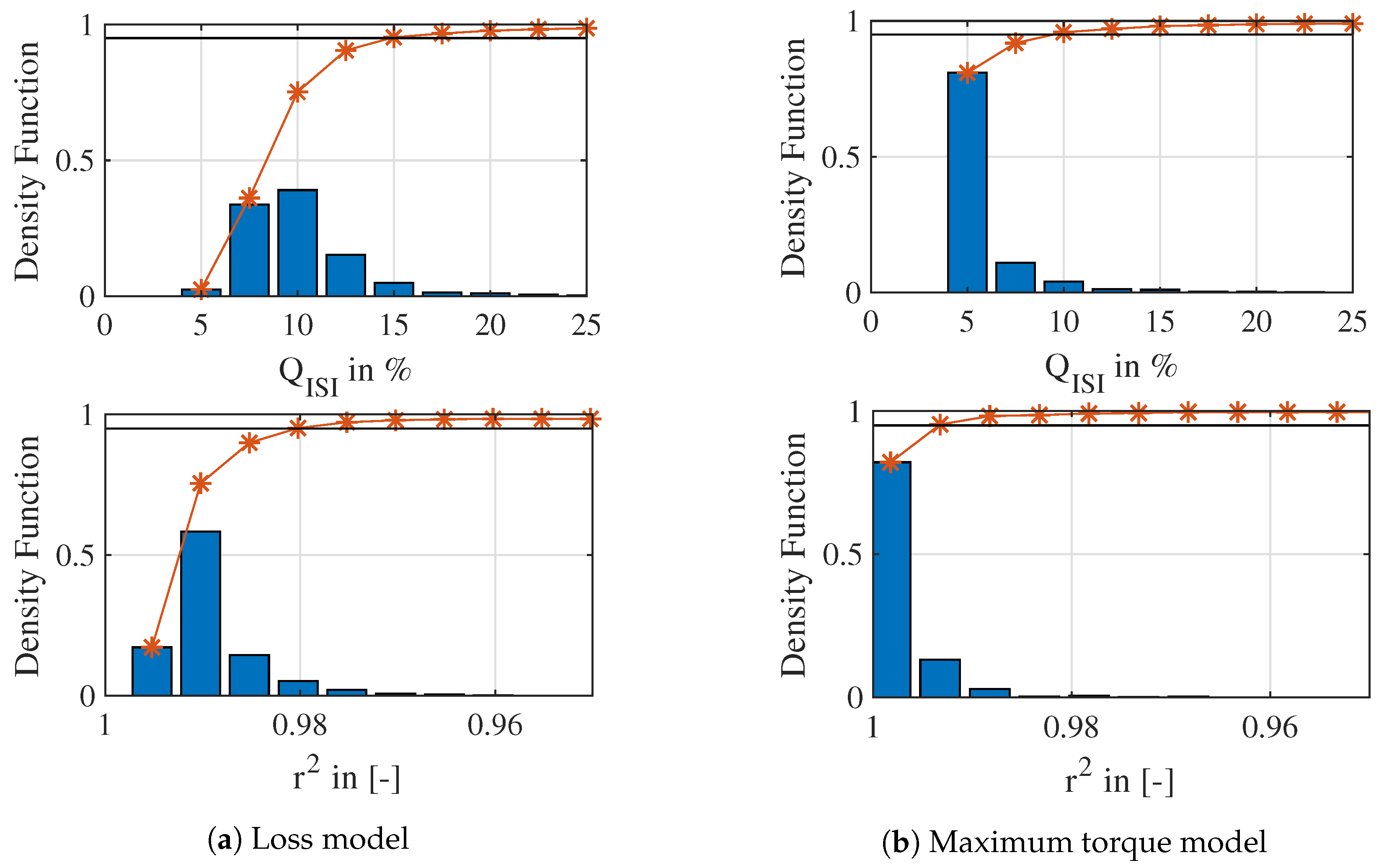The resulting statistical distributions for both criterion are given in Figure 4.

Regarding the loss model, most of the investigated designs achieve a $Q_{\mathrm{ISI}}$ between 7% and 12% as can be seen in Figure 4a. As indicated by the intersection between the cumulative density and the horizontal black line, 95% show values better than 15%. Figure 4a also presents the coefficient of determination achieved with the loss model. Most designs are found to predict the losses with an accuracy around 0.99. A value better than 0.98 is observed for 95% of the investigated designs.

The interpolation stability index of the maximum torque model can be found around 5% for most of the investigated designs, as Figure 4b demonstrates. A $Q_{\mathrm{ISI}}\le 10\%$ is observed for 95% of the designs. The achievable coefficient of determination is also plotted in Figure 4b. More than 80% show an $r^2$ around 0.998, and 95% of the designs are better than 0.993.

The results demonstrate the good accuracy of the polynomial model. Even for a variation of many design variables—such as geometry, winding, electric, and material parameters—the model shows a good robustness. The results allow the usage of the model within a system-level design optimization. In order to further investigate the influence of the occurring modelling error on the $C{O}_2$ emissions, a consumption simulation is conducted, and the results of the polynomial model are compared to those with the FE-calculated loss map and maximum torque curve. To investigate the worst case scenario, a design with greater modelling error is chosen. During the fitting process, this design shows for the loss model $Q_{\mathrm{ISI}}=13.6\%$/$r^2=0.9878$ and for the maximum torque model $Q_{\mathrm{ISI}}=7.1\%$/$r^2=0.9968$. The resulting relative deviation in $C{O}_2$ emissions is calculated with

$$\Delta C{O}_2=\frac{∥C{O}_{2,\mathrm{FEM}}-C{O}_{2,\mathrm{Model}}∥}{C{O}_{2,\mathrm{FEM}}}·100.$$

(20)

In Figure 5, the results are plotted for different driving cycles. In all cases, the modelling error in the EDS model leads to only small deviations in $C{O}_2$ emissions, far below 1%.

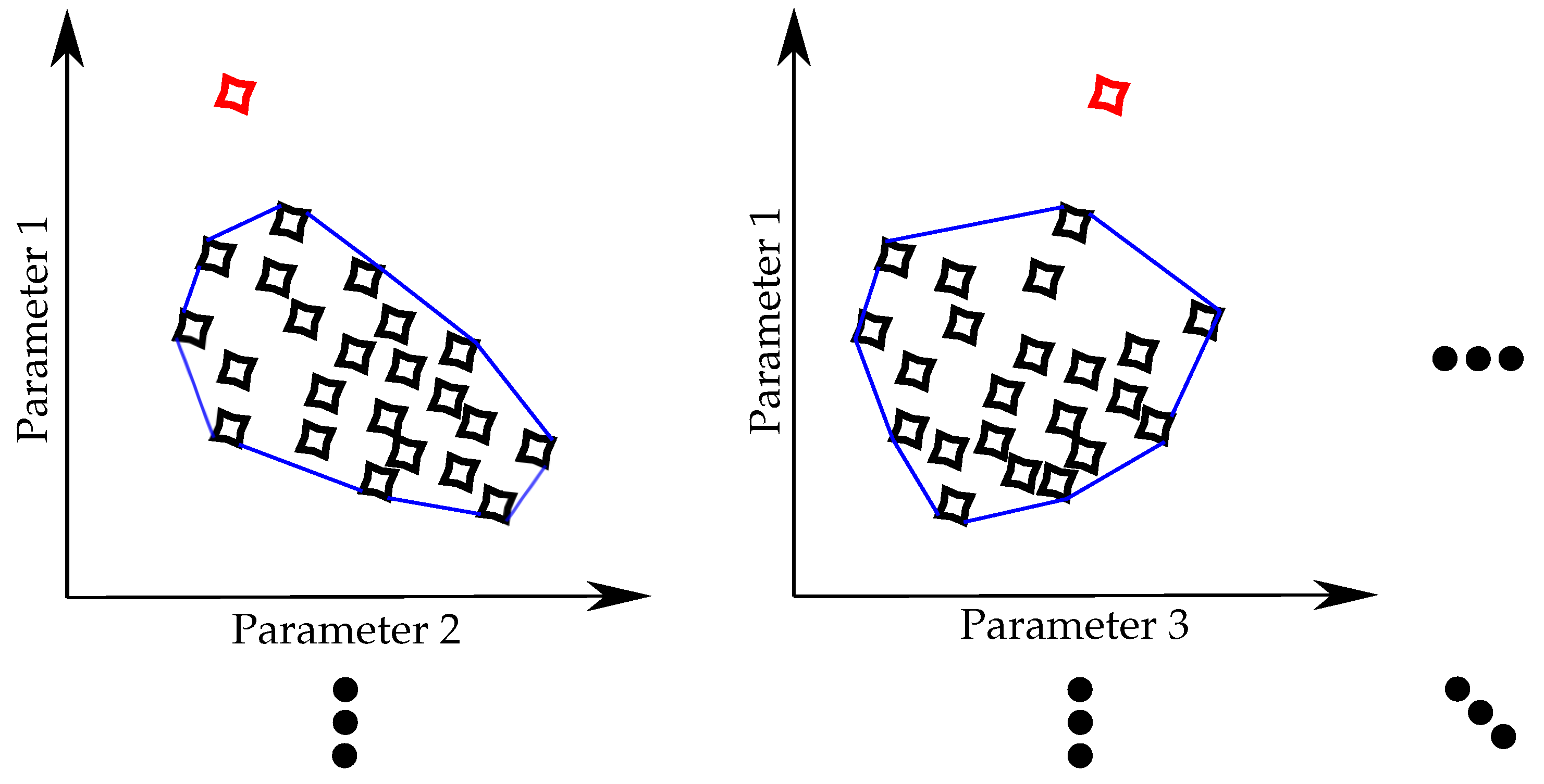
In the following, the limiting function is constructed based on the obtained 16 parameters of the polynomial model. Designs showing a bad fit are eliminated in order to guarantee a good quality of the model. The maximum allowable error is chosen as to allow most of the designs to contribute to the models and is presented in

Table 4. Maximum allowed modelling error to contribute to the limiting function.

Statistic	Loss Model		Maximum Torque Model
	${\mathit{Q}}_{\mathrm{ISI}}$	${\mathit{r}}^{\mathbf{2}}$	${\mathit{Q}}_{\mathrm{ISI}}$	${\mathit{r}}^{\mathbf{2}}$
Worst allowed value	15%	0.98	10%	0.99

. Furthermore, outliers are eliminated to prevent large white spaces within the convex hull limiting function (cf. Figure 3).

5.2. HEV System Optimization

In the first step, the ANN predicting the $C{O}_2$ emissions is validated. To do so, the predicted values $\widehat{z}$ are compared to the calculated values z by applying the statistics $Q_{\mathrm{ISI}}$ and $r^2$ in Equations (18) and (19). This time, the variable z denotes the $C{O}_2$ emission obtained by the consumption simulation, and $\widehat{z}$ the emissions obtained with the ANN model. For both investigated topologies, the achieved accuracy of the $C{O}_2$ models is shown in

Table 5. Validation statistics of the $C{O}_2$ model.

Statistic	Urban		Road		Motorway 150
	P2	P4	P2	P4	P2	P4
$Q_{\mathrm{ISI}}$	1.33%	1.61%	0.70%	0.93%	0.33%	0.55%
$r^2$	0.9799	0.9554	0.9643	0.9852	0.9430	0.9259

. It allows the consumption simulation to be replaced within the global optimization.

Finally, the optimization scheme in Figure 2 is run two times for different topologies. During the first optimization, the EDS parameters are varied in the P2 position. The second one optimizes a P14 topology, where the parameters in the P4 position are varied. Both procedures are started with an identical start population. Figure 6 presents the resulting Pareto charts. The $C{O}_2$ reduction potential is defined as a percentage of the conventional vehicle’s emission

$$\Delta C{O}_2=\frac{C{O}_2-C{O}_{2,\mathrm{conv}}}{C{O}_{2,\mathrm{conv}}}·100,$$

(21)

and represents the weighted average of the three investigated driving cycles. For this study, an equal weight for all cycles is chosen.

A weighted reduction potential of up to 28% can be achieved with a P2 hybrid. Most of this potential can already be covered with an installed mechanical EDS power of 20–25 kW. In contrast, the P4 hybrid further increases this potential with up to a 34% $C{O}_2$ savings. Again, an installed mechanical EDS power of 20–25 kW is necessary to cover most of the reduction potential. The large variance in the $C{O}_2$ savings of up to 15% for a constant EDS power results from the varying EDS characteristic. This underlines the importance of investigating not only the EDS power but also the entire EDS characteristic.

The developed approach in this paper further allows conclusions on the optimal EDS characteristics for a specific application. The sensitivity between the 16 EDS parameters and the fuel consumption can be investigated by taking a closer look at the evolution of the parameter range during optimization. Based on expert knowledge, conclusions on the application-specific optimal electromagnetic design can be extracted. 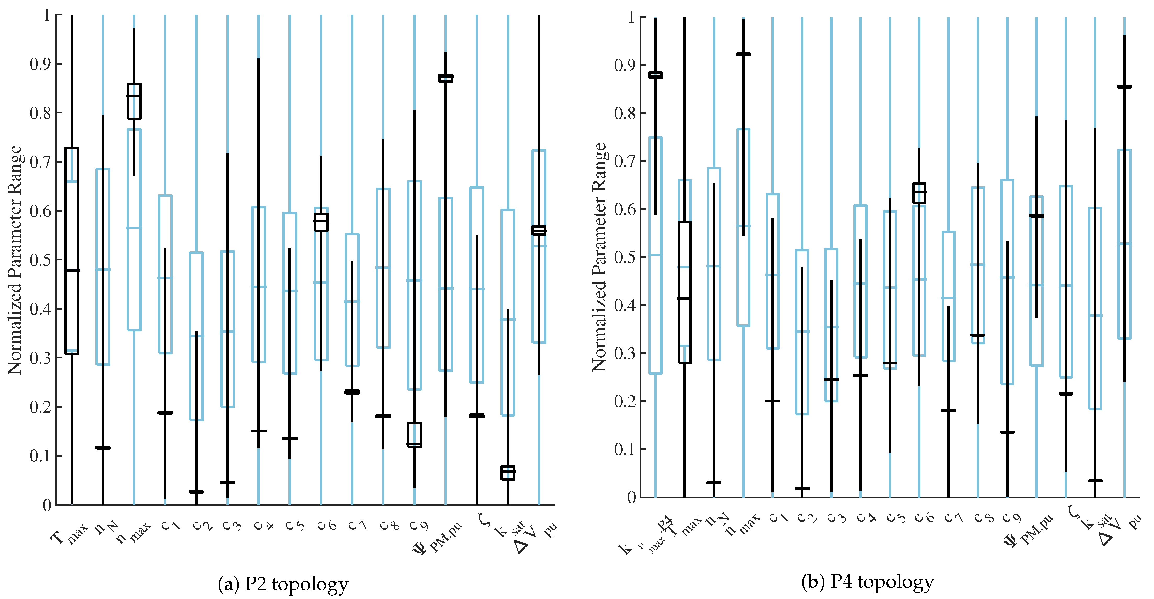Figure 7 presents the parameter range of the variation parameters and compares the optimal last generation against the random start population. The values are normalized with regard to the maximum and minimum values. The statistic boxplot representation is chosen to visualize the optimizer’s path. The box includes the 25th to 75th percentile. By comparing the start population against the last generation, a contraction of the boxes can be observed, and the parameter range is concentrated to a specific optimal region. The optimal parameter ranges, eventual interdependencies between several parameters, and their impact on the electromagnetic design are discussed in the following.

For both topologies, the nominal speed $n_{\mathrm{N}}$ shows minimal values. Especially in the P4 position, a minimal nominal speed seems to be optimal. A low nominal speed enables the maximum power at low speed, which explains this behaviour. The missing multi-gear transmission in the P4 position further increases the need for a small nominal speed. This allows one to conclude that an optimal drive in the P4 position will require a higher torque capability and therefore more active volume compared to an equally powered optimal drive in the P2 position. Having a minimal nominal speed, the maximum torque $T_{\max }$ ensures the variation in mechanical EDS power. Therefore, the torque shows a broad variation range. In contrast to the nominal speed, the maximum EDS speed $n_{\max }$ is optimally maximized. In the case of the P4 position, the additional parameter $k_{\mathrm{v},\max ,\mathrm{P}4}$ has been introduced. Comparable to the maximum speed, this decoupling coefficient also tends to higher values, although it is not at its maximum for most designs on the final Pareto front. The maximum engaged speed is proportional to the product of maximum speed and decoupling coefficient and should be large enough to gather most of the recuperation energy at high vehicle velocity. For higher speeds, it is more efficient to decouple the electric machine due to the increasing EDS losses at higher speed.

As could be expected, the optimizer tries to minimize the loss coefficients $c_1$–$c_9$ to increase the $C{O}_2$ savings. The only loss coefficient which is not minimized is the coefficient $c_6$ responsible for the asymmetric behaviour in motoring and generating mode. However, decreasing loss coefficients will require an increase in active volume, which will imply an increase in cost and installation space. Whereas the speed dependent coefficients $c_1$ and $c_2$ are minimized for both topologies, the torque dependent coefficients $c_3$ and $c_4$ seem to be more important in the P2 position. While a decreasing coefficient $c_3$ can be achieved by a higher power factor and therefore an increasing magnet flux contribution ${\mathsf{\Psi }}_{\mathrm{PM},\mathrm{pu}}$, a higher amount of copper will lead to a decreasing coefficient $c_4$. The loss coefficient $c_7$ highly influencing the no-load losses in the field-weakening region is more important in the P4 position. Since the physical meaning of this coefficient is coupled to the field-weakening effort, the smaller values for $c_7$ require a smaller magnet flux contribution ${\mathsf{\Psi }}_{\mathrm{PM},\mathrm{pu}}$. Such coupling effects between the different EDS parameters are achieved due to the limiting function. In contrast, the optimal magnet flux contribution in the P2 position is relatively high, leading to less magnetizing current and therefore smaller coefficients $c_3$ and $c_4$. The general minimization of the loss coefficients leads to less utilized machines and therefore to low saturation values $k_{\mathrm{sat}}$.

From the Pareto front in Figure 6, one optimal design is chosen by weighting the objectives $\Delta C{O}_2$ and $P_{\mathrm{eds},\max }$ at the ratio of 2 to 1. The related EDS characteristics are plotted in Figure 8. By comparing the efficiency maps, the same correlations as before can be observed. A good efficiency around zero torque seems to be optimal for both investigated parallel hybrid topologies. In a P2 position, a good efficiency at low speed and higher torque is beneficial, since the gear box maintains the operating speed within a restricted area. In a P4 position, the EDS speed is coupled to the vehicle’s velocity. Good efficiencies are then required at a higher speed and low torque.

As the previous results demonstrated, the newly developed data-enhanced EDS model allows a detailed and comprehensive investigation on the optimal EDS characteristics for different specific applications. One minor weakness of the polynomial loss model can be observed in Figure 8. The optimizer tends to choose relatively high values for the loss coefficient $c_6$ responsible for the asymmetric behaviour between motoring and generating mode. This leads to a slightly stronger asymmetry than expected. In order to keep the coefficient $c_6$ in check, some caution has to be paid to the limiting function and the database it is constructed from. The size of the database is especially an important factor and should be chosen with care.

6. Conclusions

This paper discusses the open research issue of considering the EDS characteristic during system-level component sizing in multi-drive systems. Different methods for sizing are reviewed and discussed. A new data-enhanced EDS model is proposed. The new model is capable of varying all relevant parameters including torque, nominal speed, and level and shape of the EDS efficiency. Once a database is available, the model has good properties regarding accuracy, scalability, and computational effort. However, a robust and valid limiting function is crucial, since the optimizer will enter every possible gap.

The new approach is applied to an HEV system optimization of a parallel hybrid in the P2 and P4 positions. A large influence (up to 15%) of the EDS characteristic on the $C{O}_2$ reduction potential is observed. This allows for the conclusion that the EDS characteristic should be considered during system-level component sizing. Furthermore, a dependency of the optimal EDS characteristic on the considered topology is found. In the case of multi-drive systems, the usage of identical electric drive systems independent of the installation position might be sub-optimal in terms of vehicle energy consumption.

Further work may include the application of the new approach to serial or power-split hybrids. Moreover, an adaption of the polynomial model to other machine types such as induction machines or electrically excited synchronous machines would allow for a more detailed investigation on the optimal EDS characteristics.