Abstract
The aim of this paper is the development of a 7-DOF (Degrees Of Freedom) mathematical model of an IndyCar and the implementation of an Artificial Neural Network in order to predict the optimal setup parameters of the car, reducing time and costs for race teams. The mathematical model is created by using MATLABTM and Simulink software starting from a telemetry acquisition at the Houston circuit and is based on Vertical Vehicle Dynamic equations. The optimal setup parameters have been predicted through an Artificial Neural Network (ANN) by using the NFTOOL Toolbox of MATLABTM software. ANN is implemented in a Quarter Car model, firstly, in order to train the network and predict the parameters able to reduce tire deflection and suspension travel in the time domain and the resonance peaks amplitude in the frequency domain. Then, it is implemented in the 7-DOF model in order to predict the best setup parameters able to reduce body movements and the weight transfers of the car.
1. Introduction
The evaluation of the best qualifying setup of a race car is one of the hardest and important tasks of a race team. In this regard, the mathematical modeling of a vehicle suspension system can be very helpful for engineers to understand the behavior of the car during a lap. The simplest configuration is the Quarter Car model, which is commonly used in the literature [1], to study, in first approximation, the response of a suspension system to a road input. Despite the fact that the model is easily understood and of simple application, it presents important limitations:
- It only takes into consideration the heave motion of the system without studying the body motion of the roll, pitch and yaw;
- The system is assumed to be linear but in reality, considering for example the shock absorbers or the bump stops characteristics, is strongly nonlinear;
- It does not take into consideration the geometrical effect of having four wheels.
For this reason, many authors have developed more complex models in order to evaluate the complex suspension system movement [2,3,4].
In Motorsport, the constant evolution of suspension systems and tire technology makes it more complicated to evaluate the best setup parameters for a certain track. Moreover, in order to contain time and costs, the FIA limits days available for the race teams for on-track acquisition. Hence, in adding to mathematical models, during test periods, race teams use the Post Shaker Rig in order to find the best suspension setup. Basically, a Post Shaker Rig is a system able to replicate the telemetry acquisition data through actuator displacement. The simplest configuration is the Four Post Shaker Rig, consisting of four actuators placed under each wheel and able to reproduce the road profile of the track. In the past, the race teams used the Four Post Shaker Rig for indoor testing [5]. The Seven Post Shaker Rig has, in addition, three aeroloader actuators, two of these placed on the rear side of the car and the third placed on the front side of the car. Therefore, the Seven Post is also able to reproduce the body movements: roll, pitch and heave [6,7,8].
Moreover, it is possible to find the Eight Post Shaker Rig, which presents four aeroloaders [9]. However, as a matter of fact, the use of the Post Shaker Rig involves time and costs related to the transport of the car and the simulation of the track. For this reason, the aim of this paper is to use artificial intelligence to predict the optimal setup parameters of the car, reducing time and costs for the race teams. The starting point of the work is the mathematical modeling of the vehicle. Two models are used for characterizing vehicle behavior: the Quarter Car model and the 7-DOF model. A Quarter Car model, considering its simplicity, was used to test and train the network choosing an optimal population size [10]. Then, the 7-DOF model was used for studying the behavior of an IndyCar during a qualifying lap at the Houston circuit. Finally, the neural network is implemented in the model in order to predict the best setup parameters able to reduce roll angle, pitch angle, sprung mass heave and total weight transfer, improving grip [11] and performance.
2. Theoretical Background
In this section, the theoretical key points are analyzed, focusing in particular on:
- What is meant by setup parameters, and which ones are available for this study;
- The mathematical relation between the setup parameters and the information we can extract to characterize the behavior of a vehicle during a lap;
- The effects that change these parameters have on vehicle performance.
2.1. Setup Parameters
Basically, setting a vehicle consists of changing all the parameters that affect the vehicle behavior during a lap. For example, lowering the Center Of Gravity Height (COG) reduces load transfer and increases grip. Changing roll centers has an effect on overall roll and balance. The anti-roll bar stiffness adjustment has an effect on the understeer and oversteer behavior of the car. Damper adjustment has an effect on vibration and transient handling of a vehicle. In this work, setup parameters were chosen according to the available vehicle parameters, as shown in Table 1.

Table 1.
IndyCar parameters.
Moreover, roll center variation, spring and damper characteristics have been provided, as shown in Figure 1, Figure 2, Figure 3, Figure 4, Figure 5 and Figure 6.
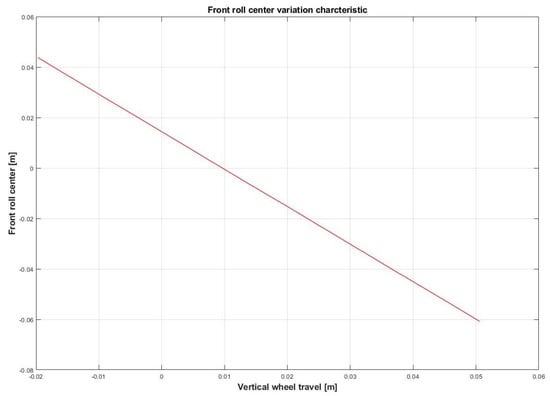
Figure 1.
Front roll center variation characteristic.
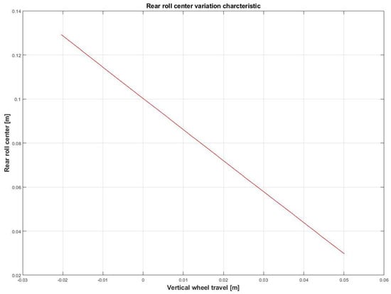
Figure 2.
Rear roll center variation characteristic.
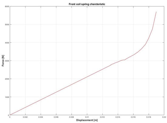
Figure 3.
Front coil spring characteristic.
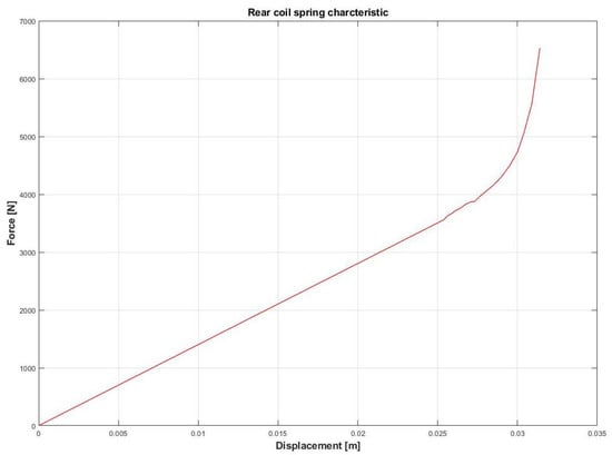
Figure 4.
Rear coil spring characteristic.
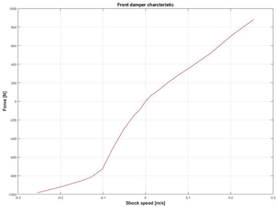
Figure 5.
Front damper characteristic.
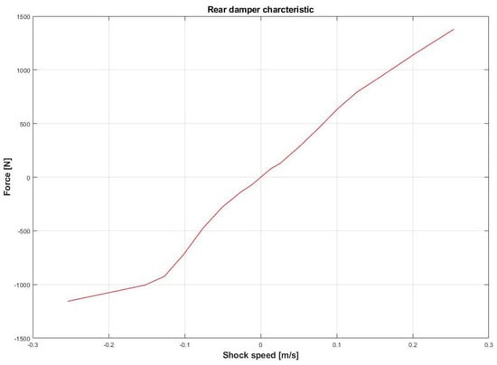
Figure 6.
Rear damper characteristic.
Among all available data, those representing the starting setup, called from now on the baseline setup, have been chosen (Table 2).

Table 2.
Parameters chosen for the baseline setup.
In addition, roll center variation, damper and spring characteristics have been chosen for the baseline setup. The choice of baseline setup parameters are due to the following considerations:
- After the chassis is manufactured, its geometry cannot be changed. For this reason, it is not possible to change the wheelbase, track width and all the other parameters related to vehicle geometry;
- Tires are imposed by the regulation; hence, it is not possible to change all the parameters related to the tire, such as tire stiffness and damping;
- Motion Ratio (MR) is a characteristic provided by the manufacturer and cannot be changed.
2.2. Quarter Car Model
The Quarter Car model represents the simplest mathematical model to study, in first approximation, the suspension motion due to a road input. It consists of a sprung mass , a spring represented by a constant stiffness k, a damper represented by a constant damping c, an inverter represented by a constant inheritance b (this element is not always present), an unsprung mass and another constant stiffness p, which represents tire vertical stiffness. In Figure 7, the Quarter Car model proposed by Guiggiani [1] and adopted in this work is shown.
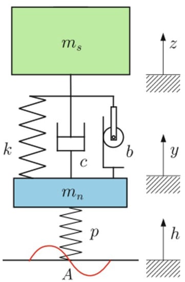
Figure 7.
Quarter Car model.
2.3. 7-DOF Model
Available vehicle parameters have been used to build a 7-DOF mathematical model based on vertical vehicle dynamic equations. As proposed by Guiggiani [1], parameters are linked together through the equilibrium equations, which are a link between forces or couples and acceleration, constitutive equations and congruence equations, which are purely geometrical links between coordinates.
The equilibrium equations are:
The constitutive equations are:
The congruence equations are:
In Figure 8 a schematic representation of a 7-DOF mathematical model is shown:
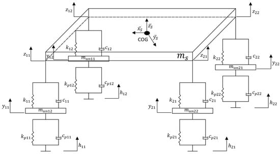
Figure 8.
7-DOF mathematical model.
2.4. Grip Effect
The main function of the tires is to convert the vertical load into two planar forces and . The variation of these planar forces during a lap represents the Contact Patch Load Variations (CPLV). Grip is influenced by the CPLV because every peak of load at the contact patch brings subsequent unloading of the tire, which compromises both the average load acting on the tire in time and the grip generation through the hysteresis mechanism at the contact patch. Hence, the grip is related to the weight transfer and also to the body movements: roll, pitch and heave. Figure 9 [11] summarizes all these concepts.
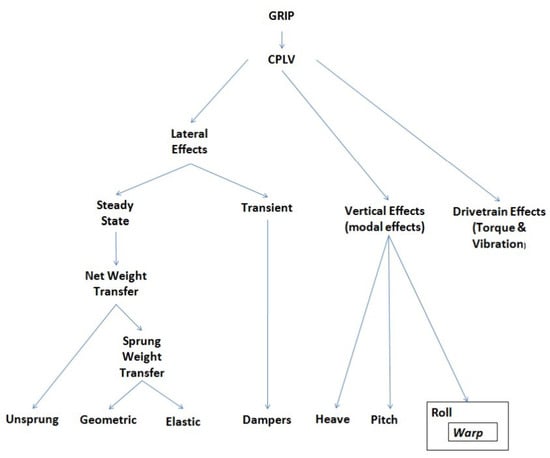
Figure 9.
The performance of the vehicle is related to the grip between road and tire. Improving the grip means decreasing the CPLV, which depends on weight transfer and body movements of roll, pitch and heave.
Moreover, the longitudinal weight transfer given by (28) is taken into consideration:
Hence, the total weight transfer is given by (29):
3. Related Work
The application of artificial intelligence to vehicle dynamics is, nowadays, a field under development. The literature review shows that the main application of a neural network is related to the prediction of the suspension response to an external input and identification of the optimum suspension parameters. Guarneri et al. [12] demonstrated that a Neural Network (NN) model can be effectively applied as a part of vehicle system model to accurately predict elastic bushings and tire dynamics behavior. Guclu and Gulez [13] investigated the time and frequency response of an 8-DOF nonlinear model due to road disturbance. In this case, the NN model predicts seat vibrations with almost zero error between desired and achieved outputs. Safari et al. [14] implemented a deep neural network algorithm on a 7-DOF model full car suspension system for the identification of an Active Vehicle Suspension response. Nagarkar et al. [15] used an Artificial Neural Network (ANN) to predict with high accuracy the optimal suspension parameters of a Mcpherson strut suspension system. In this work, the authors modeled the Mcpherson suspension with a Quarter Car model using a MATLAB/SimulinkTM environment. The suspension system has been optimized using a genetic algorithm for an objective function, in order to improve ride comfort. Finally, two optimal values of stiffness and damping were found that satisfied the objective functions. The results are then validated using an experimental test rig. After the optimization, ANN is implemented in the model using the NFTOOL Toolbox of MATLABTM, in order to predict the optimal suspension parameters. Results show that simulation, experimental and predicted values are in strong correlation and ANN is able to predict with high accuracy the optimum suspension parameters.
4. The Proposed Method
The mathematical modeling represents an important step for the understanding of a vehicle’s behavior during a lap. Although the mathematical model represents an approximation of the real behavior of the car, it is possible to obtain important information about vehicle performance. Moreover, through the equations set, it is possible to understand which variables influence comfort and performance, etc. According to a literature review, the authors developed increasingly complex models to better characterize the behavior of a vehicle. Sun et al. [2] developed a 4-DOF vehicle model for studying the pitch and bounce of the sprung mass and the bounce of the front and rear wheel response to a step input. The work shows that the different values of the dynamic index, mass ratio, weight distribution and flat ride tuning affect ride frequency and vibration isolation of the system. DUMITRIU [3] developed a 3D car 7-DOF model in order to study wheel-road adherence and passenger comfort, remarking that the usage of a different shock absorber influenced both adherence and comfort. Setiawan et al. [4] developed a 14-DOF model, including yaw motion and wheel spin. The model under examination consists of a ride and handling model. The ride model is a 7-DOF used for studying the ride performance parameter. The handling model is a 7-DOF model that takes into account longitudinal, lateral and yaw motion of the vehicle body and the four wheel spin. Moreover, the authors investigated the effect of slip and camber angle on the lateral force generated at the wheel. The model is then validated using a Step Steer Test comparing the simulation result with the experimental one. Among all developed models, in this study, the attention is focused on a Quarter Car model and a 7-DOF model. At first, the response of the Quarter Car model to a road input has been studied. In particular, from Equations (1) and (2), knowing road input, stiffness coefficient and damping coefficient, it is possible to evaluate tire deflection and suspension travel . Then, two optimal values of stiffness and damping coefficient were chosen in order to improve the response of the model. The result was analyzed both in time and frequency domains. Then, ANN was implemented in the model using the NFTOOL Toolbox of MATLABTM in order to predict the optimized values. Finally, a comparison between optimized and predicted values was carried out. After the ANN was tested and validated with the Quarter Car model, the same methodology was applied to the 7-DOF model. In this case, the parameters being optimized are the baseline setup parameters. The optimization or, in general, setup adjustment are carried out by a human factor before the race, changing, for example, mass distribution and stiffening or softening suspension elements. Then, the influence of changing parameters on body movements (roll, pitch and sprung mass vertical travel) and load transfer were studied. This has been undertaken because an improvement of these responses leads to an improvement in vehicle performance [11]. In addition, the study was carried out both in time and frequency domains. Then, ANN was implemented in the model in order to predict the optimized setup parameters. In the end, a comparison between baseline, optimized and predicted values was carried out.
5. Empirical Research Methodology
The first step of the work was the creation of a 7-DOF model of an IndyCar. The vehicle can be seen as a transfer function in which a set of input data produces a response of the system, basically the 7-DOF. Input and output variables are related through equilibrium, constitutive and congruence equations, as already mentioned in Section 2.3. Input data are real telemetry acquisitions from the Houston circuit in Texas, which usually hosts the NTT IndyCar Series (Figure 10).
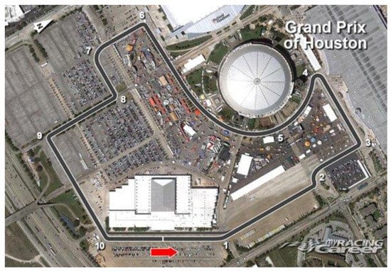
Figure 10.
Houston circuit in Texas, USA.
The available data are accelerations along three axis and damper travels, which represent the model inputs (Figure 11 and Figure 12).
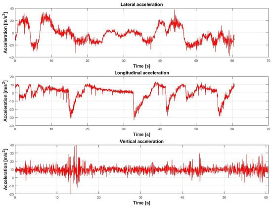
Figure 11.
Lateral, longitudinal and vertical acceleration vs. time.
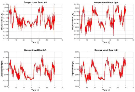
Figure 12.
Damper travels vs. time.
From the equation sets, it is possible to evaluate the 7-DOF of the model, as shown in Table 3.

Table 3.
Output of the 7-DOF model.
In addition, from the previous considerations about vehicle performance, total weight transfer was evaluated. The equation sets were solved using the SimulinkTM environment (Figure 13). The simulation time is equal to the acquired lap time at the Houston circuit, and the time step is 0.001 s.
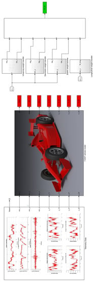
Figure 13.
Simulink model of an IndyCar. Red blocks are the outputs of the model, and the green block is the total weight transfer.
An Artificial Neural Network was implemented in the mathematical model using the NFTOOL Neural Network Toolbox of MATLABTM. The Toolbox provides algorithms and pre-trained models to create, train, simulate and visualize neural networks. The chosen Artificial Neural Network is a feed-forward network in which the unidirectional information comes from input data to target data. The network was implemented in a Quarter Car model, firstly, in order to predict the parameters able to reduce tire deflection and the suspension travel in the time domain and frequency domain. This choice was made in order to test the goodness of optimal parameters prediction. The designated parameters of the optimization are suspension spring rate k and damping rate c (Figure 7). The search space for the optimization is k ∈ ± for the stiffness coefficient and c ∈ ± for the damping coefficient. In this case, “baseline” terminology is used to indicate initial parameter values. In order to train the network, a series of 40 simulations was carried out in SimulinkTM, varying spring rate and damping rate values inside the search space. Hence, the population size is 40 elements for both the input and output layers. Network topology consists of two input layers, represented by suspension travel and tire deflection population, and two output layers represented by stiffness and damping rate population. The hidden layer contains the artificial neurons, in this case the same number as the population size. The ANN topology is shown in Figure 14.
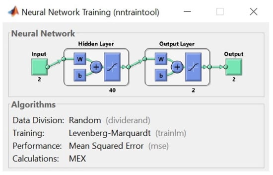
Figure 14.
ANN topology for the Quarter Car model optimization. Input layer contains suspension travel and tire deflection population. The output layer contains the designated variables of the optimization, spring rate and damping rate. The hidden layer contains the artificial neurons.
After training the network with a simple Quarter Car model, it is possible to extend the same procedure to the 7-DOF model. In this case, the parameters to optimize are: roll angle, pitch angle, sprung mass vertical travel and total weight transfer. The designated parameters of the optimization are the center of gravity height h, rolling stiffness on front axle , rolling stiffness on rear axle , roll center variation characteristic on front and rear axle, coil spring characteristic on front and rear axle and shock absorber characteristic on front and rear axle, as previously mentioned in Section 2.1. The search space for the optimization is the same of the Quarter Car model for all the variables. The family of training data was created through 100 subsequent simulations in SimulinkTM with different setup parameters, following the search space. Then, both output and input values were saved in a matrix to create the neural network. In particular, the input matrix (which contains the variables to optimize) is a while the target matrix (which contains the different setup configuration) is a . Hence, the topology of the network consists of:
- Four input layers: roll angle, pitch angle, sprung mass vertical travel and total weight transfer vectors;
- Two-hundred-and-forty-five output layers: contains, in order, the vectors of the designated optimization variables;
- Hidden layer: 100 neurons.
The ANN topology is shown in Figure 15.
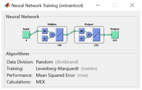
Figure 15.
The ANN topology for the 7-DOF model optimization. The input layer contains the variable to optimize: roll angle, pitch angle, sprung mass vertical travel and total weight transfer. The output layer contains the vectors of the designated variables of the optimization. The hidden layer contains the artificial neuron.
The goodness of the optimization was evaluated through a mean squared error, which represents the network’s performance, and a correlation coefficient R between target data (simulation values) and output data (i.e., ANN output values).
6. Results
In this section, we show the results regarding the Quarter Car and 7-DOF model simulation. For what concerns the Quarter Car model, a comparison between the baseline setup and optimized setup was carried out in order to highlight the improvement of the optimized setup related to tire deflection and suspension travel, in the time and frequency domains. Then, ANN was implemented in the model in order to predict the optimal suspension parameters. The same methodology was applied to the 7-DOF model.
6.1. Quarter Car Model
Initially, the response of the Quarter Car model to a sine wave input was evaluated, as shown in Figure 16.
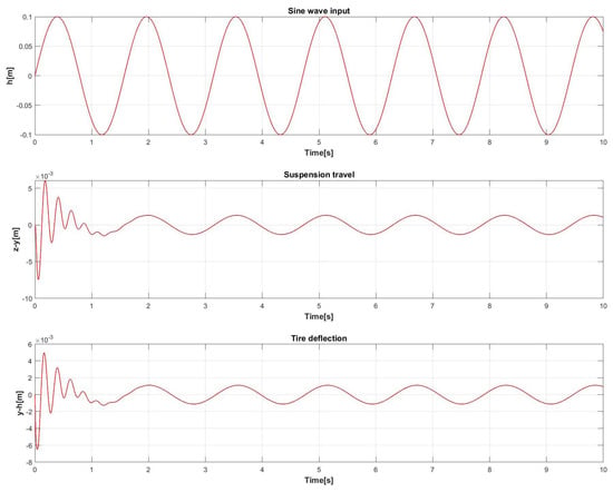
Figure 16.
Quarter Car model response in terms of suspension travel and tire deflection to a sine wave input of 0.1 m of amplitude for a 10 s simulation time.
Figure 17 shows the comparison between the baseline setup and the optimized setup for suspension travel and tire deflection in the time domain.
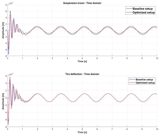
Figure 17.
Comparison between baseline setup and optimized setup. The optimized setup is able to reduce the amplitude of suspension travel and tire deflection in the time domain.
Figure 18 shows the comparison between the baseline setup and optimized setup of suspension travel and tire deflection in the frequency domain.
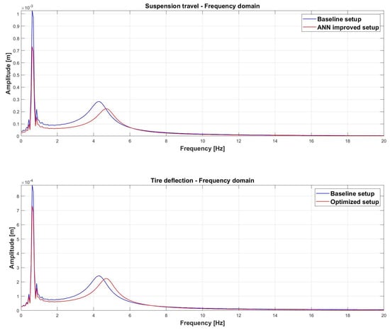
Figure 18.
Comparison between the baseline setup and optimized setup. The optimized setup is able to reduce the resonance peak amplitude of suspension travel and tire deflection in the frequency domain.
After the optimization of the baseline setup, ANN is implemented in the model in order to predict the optimized setup parameters. A neural network script was imported into the MATLABTM workspace, and the identification vector of the optimized parameters was evaluated through the following MATLABTM command:
The output of this command is a vector that contains the corresponding setup parameters. Figure 19 shows the output vector of the neural network.
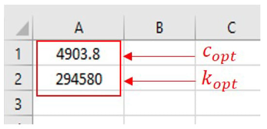
Figure 19.
Output vector of the neural network.
Table 4 shows the comparison between the baseline, optimized and predicted ANN setup for the spring and damping rate.

Table 4.
Comparison between the baseline, optimized and predicted ANN setup.
6.2. 7-DOF Model
After testing the network with a Quarter Car model, roll angle, pitch angle, sprung mass vertical travel and total weight transfer of the 7-DOF model were optimized. Figure 20 shows the trend of the roll angle for the baseline and optimized setup in the time domain.
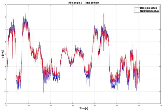
Figure 20.
Comparison between the baseline provided setup and improved setup for the roll angle trend in the time domain.
Figure 21 shows the trend of roll angle for the baseline and optimized setup in the frequency domain.
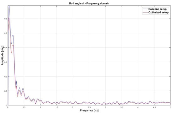
Figure 21.
Comparison between the baseline provided setup and improved setup for the roll angle trend in the frequency domain.
Figure 22 shows the trend of the pitch angle for the baseline and optimized setup in the time domain.
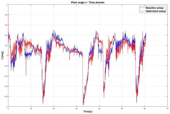
Figure 22.
Comparison between the baseline provided setup and improved setup for the pitch angle trend in the time domain.
Figure 23 shows the trend of the pitch angle for the baseline and optimized setup in the frequency domain.
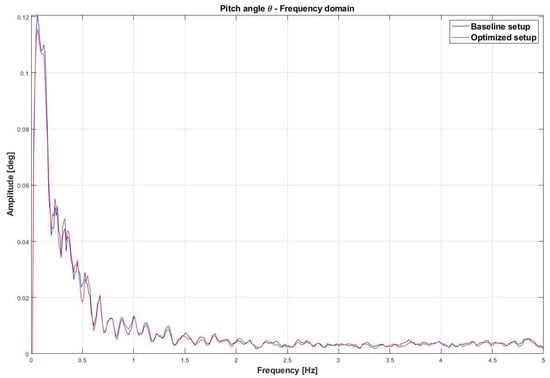
Figure 23.
Comparison between the baseline provided setup and improved setup for the pitch angle trend in the frequency domain.
Figure 24 shows the trend of heave response of the car for the baseline and optimized setup in the time domain.
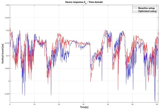
Figure 24.
Comparison between the baseline provided setup and improved setup for heave response of the car in the time domain.
Figure 25 shows the trend of heave response of the car for the baseline and optimized setup in the frequency domain.
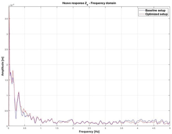
Figure 25.
Comparison between the baseline provided setup and improved setup for the heave response of the car in the frequency domain.
Figure 26 shows the total weight transfer for baseline and optimized setup in the time domain.
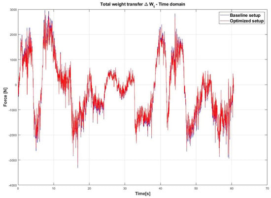
Figure 26.
Comparison between the baseline provided setup and improved setup for the total weight transfer of the car in the time domain.
Figure 27 shows the total weight transfer for the baseline and optimized setup in the frequency domain.
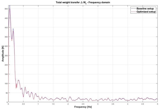
Figure 27.
Comparison between the baseline provided setup and improved setup for the total weight transfer of the car in the frequency domain.
After the optimization of the baseline setup, the ANN is implemented in the model in order to predict the optimized setup parameters. The neural network script was imported into the MATLABTM workspace, and the identification vector of the optimized parameters was evaluated through the following MATLABTM command:
The output of this command is a vector that contains the corresponding setup parameters.
Figure 28 shows the output vector of the neural network.
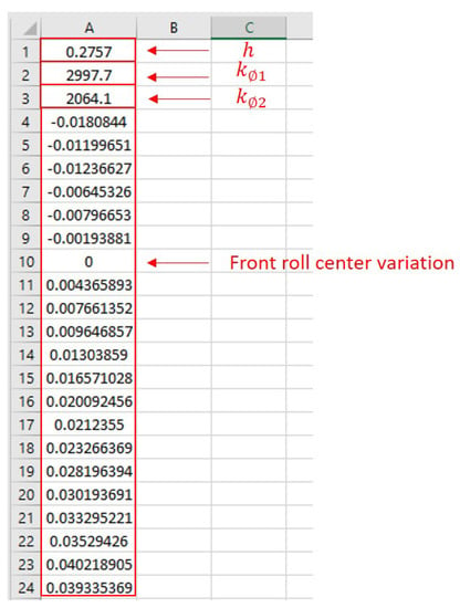
Figure 28.
Output vector of the neural network.
Table 5 shows the comparison between the baseline, optimized and predicted ANN setup for the center of gravity height and roll stiffness on the front and rear axle.

Table 5.
Comparison between the baseline, optimized and predicted ANN setup.
Figure 29, Figure 30, Figure 31, Figure 32, Figure 33 and Figure 34 show the comparison between the baseline, optimized and predicted ANN setup for roll center, spring and damper characteristics on the front and rear axle, respectively.
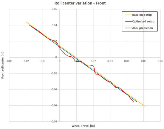
Figure 29.
Front roll center variation comparison.
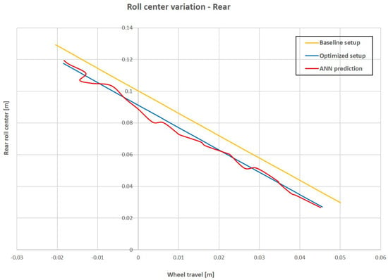
Figure 30.
Rear roll center variation comparison.
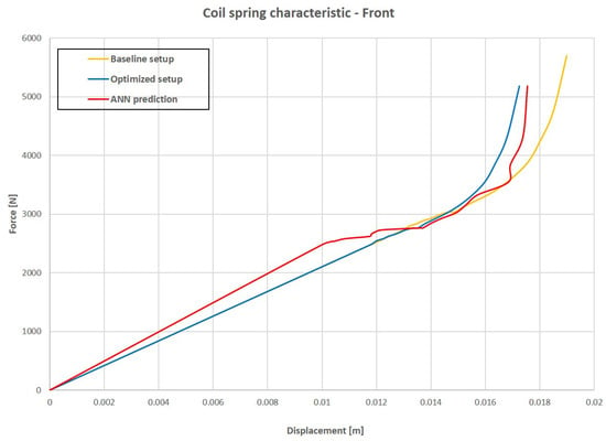
Figure 31.
Front spring characteristic comparison.
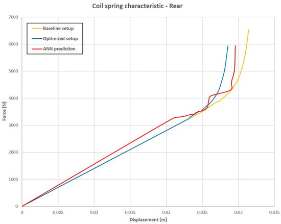
Figure 32.
Rear spring characteristic comparison.
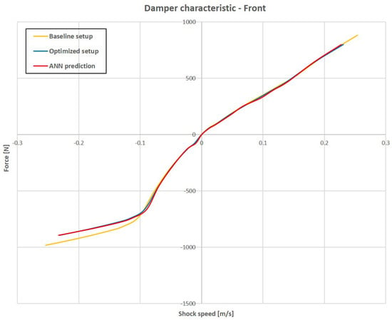
Figure 33.
Front damper characteristic comparison.
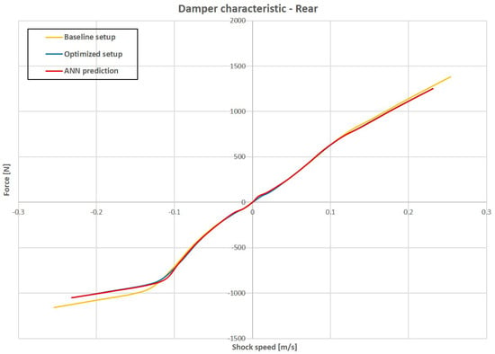
Figure 34.
Rear damper characteristic comparison.
7. Discussion
The Quarter Car model optimization shows that the spring rate and the damping rate influence suspension travel and tire deflection. In fact, as shown in Figure 17 and Figure 18, optimized setup parameters reduce tire deflection and suspension travel fluctuations in the time domain and resonance peaks amplitude in the frequency domain. The goodness of the ANN prediction of the optimized parameters was evaluated through a correlation coefficient R between target data and output data for training, validation and test, and mean squared error for the best validation performance. Considering the simplicity of the model, the best validation performance is reached after five epochs with , as shown in Figure 35.
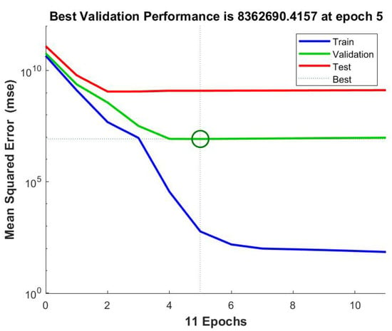
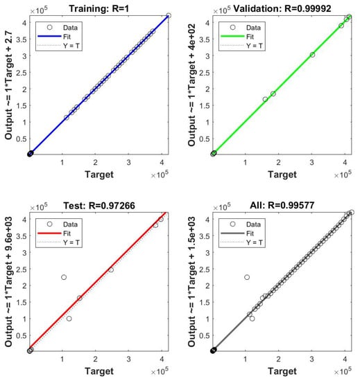
Figure 35.
Correlation coefficient R between target data and output data for training, validation and test and mean squared error for the best validation performance.
The 7-DOF model optimization shows that the optimized parameters set is able to reduce the trend of the roll angle, pitch angle, sprung mass vertical travel and total weight transfer in the time and frequency domains. Moreover, observing trends in the frequency domain, the major frequency contributions are included in the range 0–5 Hz, which is the range in which the contribution of the body movements is expected. In this case, the correlation coefficient R between target data and output data for training, validation and test and the mean squared error for the best validation performance was evaluated. The best validation performance is reached after 150 epochs with , as shown in Figure 36
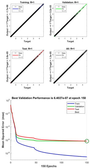
Figure 36.
Correlation coefficient R between target data and output data for training, validation and test and mean squared error for the best validation performance.
The ANN application for prediction of the optimized parameters shows a strong correlation between optimized and predicted parameters when a single value is taken into account. This fact is confirmed by the results shown in Table 4 and Table 5, in which the error between the optimized and ANN predicted setup is very low. Some difficulties emerge when characteristics are taken into account, such as roll center, spring and damper. In fact, results show that the prediction is not very accurate for the roll center and spring characteristic, while the correlation is strong for the damper characteristic.
8. Conclusions and Future Work
In this paper, the authors presented the creation of a 7-DOF mathematical model of an IndyCar, optimization of the car setup and prediction of the optimized setup parameters through an Artificial Neural Network. Starting from a telemetry acquisition at the Houston circuit, the behavior of the car during a lap was studied. In particular, the study focused on body movements and weight transfer because they are related to grip and, hence, to the car performance. Then, the influence of the optimized setup on car performance was investigated through a comparison, in the time and frequency domains, between the baseline setup and optimized setup. In the end, the ANN algorithm was implemented in the model in order to predict the optimized variables. The results show a strong correlation and high accuracy prediction of the designated parameters. At the moment, the application of artificial intelligence to vehicle dynamics is a field under development and, in this way, this study represents a novelty. The use of Seven Post is currently one of the best choices for finding the best suspension setting, despite the related costs. For this reason, future development of this work could be the creation of a virtual Seven Post, able to replicate telemetry data starting from actuator displacement. In addition, following this work, an ANN algorithm could be implemented in the model in order to try a different setup combination through the generation of a population dataset. In the end, the neural network could be able to provide an optimal setting parameter combination for a certain track.
Author Contributions
D.D.: conceptualization, supervision, validation, review and editing. G.R.: conceptualization, supervision, validation, review and editing. E.D.: methodology, validation, data curation, review and editing. A.Q.: conceptualization, supervision, validation, review and editing. D.M.: conceptualization, supervision, validation, review and editing. F.A.: formal analysis, data curation, software, writing—original draft, writing—review and editing. All authors have read and agreed to the published version of the manuscript.
Funding
This research received no external funding.
Institutional Review Board Statement
Not applicable.
Informed Consent Statement
Not applicable.
Data Availability Statement
The data presented in this study are available on request from the corresponding author. The data are not publicly available.
Conflicts of Interest
The authors declare no conflict of interest.
Abbreviations
The following abbreviations are used in this manuscript:
| m | Total vehicle mass [kg] |
| Sprung mass [kg] | |
| Front sprung mass [kg] | |
| Rear sprung mass [kg] | |
| Unsprung mass [kg] | |
| l | Wheelbase [m] |
| Front wheelbase [m] | |
| Rear wheelbase [m] | |
| Front track width [m] | |
| Rear track width [m] | |
| h | Center Of Gravity height [m] |
| Front dynamic tire radius [m] | |
| rear dynamic tire radius [m] | |
| Front no-roll center [m] | |
| Rear no-roll center [m] | |
| b | Pitch center height [m] |
| Height of no-roll axis under the COG [m] | |
| Rolling stiffness on front axle [Nm/deg roll] | |
| Rolling stiffness on rear axle [Nm/deg roll] | |
| Front Anti-Roll bar stiffness at the wheel [N/m] | |
| Rear Anti-Roll bar stiffness at the wheel [N/m] | |
| Front left spring rate [N/m] | |
| Front right spring rate [N/m] | |
| Rear left spring rate [N/m] | |
| Rear right spring rate [N/m] | |
| Front left damping rate [Ns/m] | |
| Front right damping rate [Ns/m] | |
| Rear left damping rate [Ns/m] | |
| Rear right damping rate [Ns/m] | |
| Front left tire vertical stiffness [N/m] | |
| Front right tire vertical stiffness [N/m] | |
| Rear left tire vertical stiffness [N/m] | |
| Rear right tire vertical stiffness [N/m] | |
| Front left tire vertical damping [Ns/m] | |
| Front right tire vertical damping [Ns/m] | |
| Rear left tire vertical damping [Ns/m] | |
| Rear right tire vertical damping [Ns/m] | |
| Roll inertia [kgm] | |
| Pitch inertia [kgm] | |
| Front damper motion ratio [-] | |
| Rear damper motion ratio [-] | |
| Front spring motion ratio [-] | |
| Rear spring motion ratio [-] | |
| Front Anti-Roll bar motion ratio [-] | |
| Rear Anti-roll bar motion ratio [-] |
References
- Guiggiani, M. The Science of Vehicle Dynamics: Handling, Braking, and Ride of Road and Race Cars; Springer: Amsterdam, The Netherlands, 2014. [Google Scholar]
- Sun, T.; Zhang, Y.; Barak, P. 4-DOF Vehicle Ride Model; SAE Technical Paper; SAE International: Warrendale, PA, USA, 2002. [Google Scholar] [CrossRef]
- Dumitriu, D. Car vertical dynamics 3d simulator using a 7 dof model. Acta Tech. Napoc. Ser. Appl. Math. Mech. Eng. 2012, 55, 647–650. [Google Scholar]
- Setiawan, J.D.; Safarudin, M.; Singh, A. Modeling, simulation and validation of 14 DOF full vehicle model. In Proceedings of the International Conference on Instrumentation, Communication, Information Technology, and Biomedical Engineering 2009, Bandung, Indonesia, 23–25 November 2009; pp. 1–6. [Google Scholar] [CrossRef]
- Cambiaghi, D.; Gadola, M.; Vetturi, D. Suspension System Testing and Tuning with the Use of a Four-Post Rig; SAE Technical Paper; SAE International: Warrendale, PA, USA, 1998. [Google Scholar] [CrossRef]
- Kowalczyk, H. Damper Tuning with the Use of a Seven Post Shaker Rig; SAE Technical Paper; SAE International: Warrendale, PA, USA, 2002. [Google Scholar] [CrossRef]
- Kelly, J.; Kowalczyk, H.; Oral, H.A. Track Simulation and Vehicle Characterization with 7 Post Testing; SAE Technical Paper; SAE International: Warrendale, PA, USA, 2002. [Google Scholar] [CrossRef]
- Chan, B.; Sandu, C. Development of a Virtual 7-Post Test Rig for Experimental Validation. In Proceedings of the ASME International Mechanical Engineering Congress and Exposition, Chicago, IL, USA, 5–10 November 2006. [Google Scholar]
- Southward, S.C.; Boggs, C.M. Comparison of the Performance of 7-Post and 8-Post Dynamic Shaker Rigs for Vehicle Dynamics Studies. SAE Int. J. Passeng. Cars Mech. Syst. 2008, 1, 1319–1324. [Google Scholar] [CrossRef]
- Alander, J. On optimal population size of genetic algorithms. In Proceedings of the 1992 Proceedings Computer Systems and Software Engineering, The Hague, The Netherlands, 4–8 May 1992; IEEE Computer Society: Los Alamitos, CA, USA, 1992; pp. 65–70. [Google Scholar] [CrossRef]
- Segers, J. Analysis Techniques for Racecar Data Acquisition, 2nd ed.; SAE International: Warrendale, PA, USA, 2014. [Google Scholar]
- Guarneri, P.; Rocca, G.; Gobbi, M. A Neural-Network-Based Model for the Dynamic Simulation of the Tire/Suspension System While Traversing Road Irregularities. IEEE Trans. Neural Netw. 2008, 19, 1549–1563. [Google Scholar] [CrossRef] [PubMed]
- Guclu, R.; Gulez, K. Neural network control of seat vibrations of a non-linear full vehicle model using PMSM. Math. Comput. Model. 2008, 47, 1356–1371. [Google Scholar] [CrossRef]
- Safari, A.; Mehralian, S.; Teshnehlab, M. Full-Car Active Suspension System Identification Using Flexible Deep Neural Network. In Proceedings of the 2020 8th Iranian Joint Congress on Fuzzy and intelligent Systems (CFIS), Mashhad, Iran, 2–4 September 2020; pp. 191–198. [Google Scholar] [CrossRef]
- Nagarkar, M.; Elgohary, M.; Bhalerao, Y.; Patil, G.; Patil, R. Artificial neural network predication and validation of optimum suspension parameters of a passive suspension system. SN Appl. Sci. 2019, 1, 1–17. [Google Scholar] [CrossRef] [Green Version]
Publisher’s Note: MDPI stays neutral with regard to jurisdictional claims in published maps and institutional affiliations. |
© 2021 by the authors. Licensee MDPI, Basel, Switzerland. This article is an open access article distributed under the terms and conditions of the Creative Commons Attribution (CC BY) license (https://creativecommons.org/licenses/by/4.0/).