Small Changes in Vehicle Suspension Layouts Could Reduce Interior Road Noise


Abstract
1. Introduction
1.1. Focus of This Paper
1.2. State of the Art
1.2.1. Optimizing Road Noise
1.2.2. Suspension Kinematics
1.2.3. Automated FE Model Generation
2. Methods
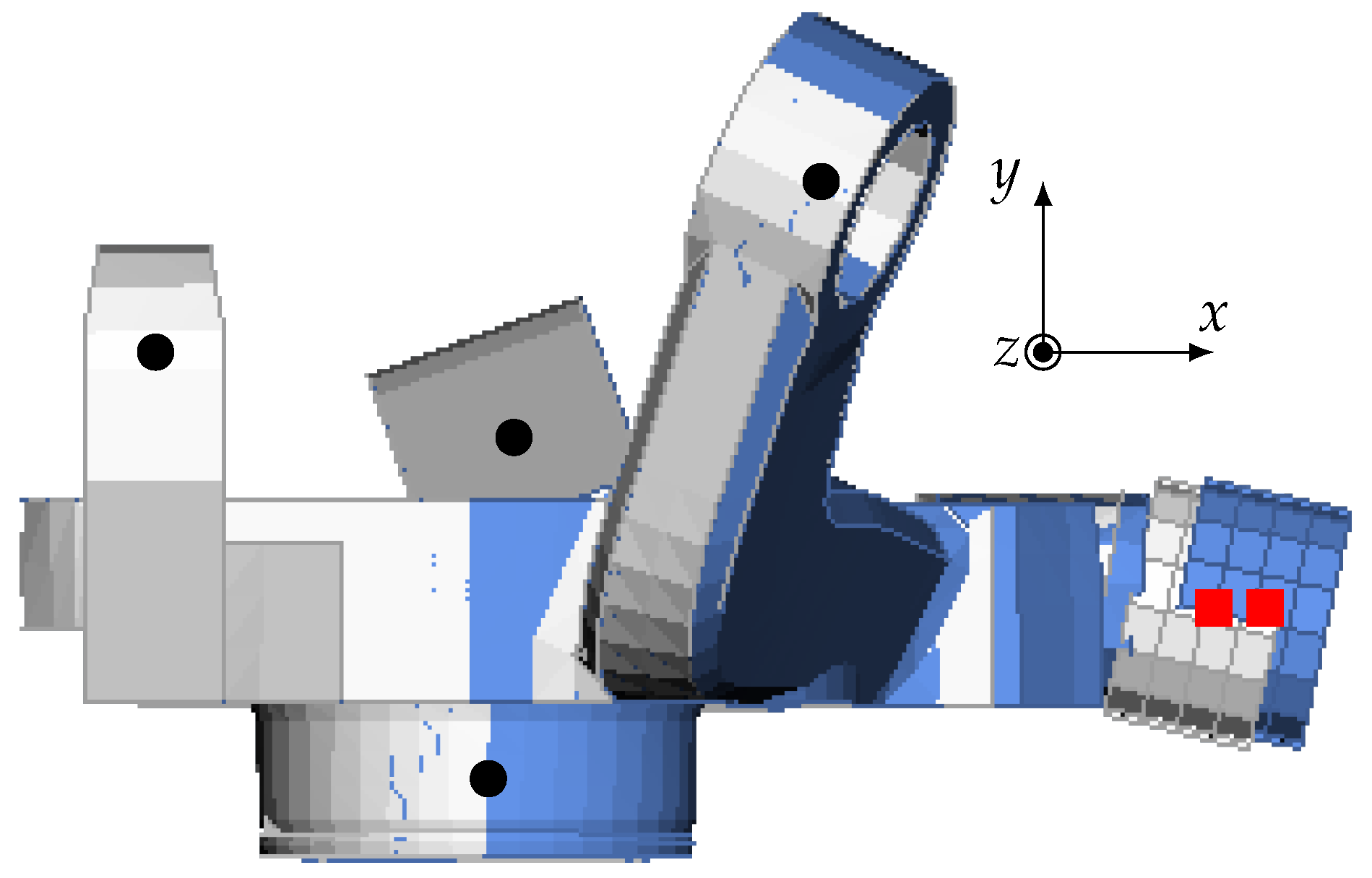
2.1. Simulation Model
2.2. Modeling Parts for Changed Kinematics
2.2.1. Modifying the Track Rod
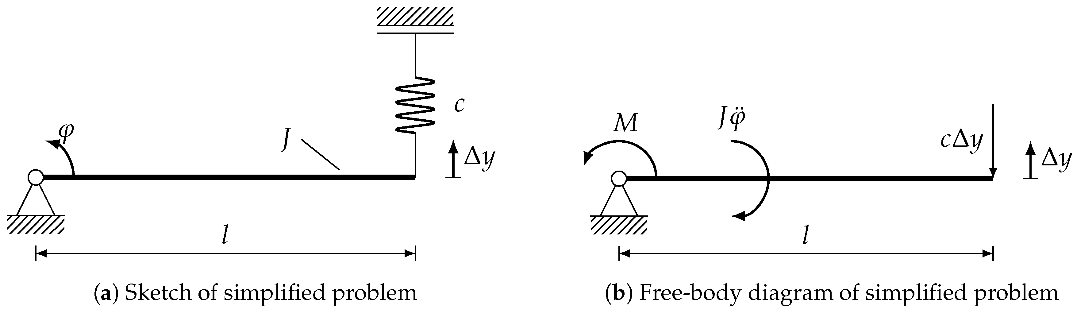
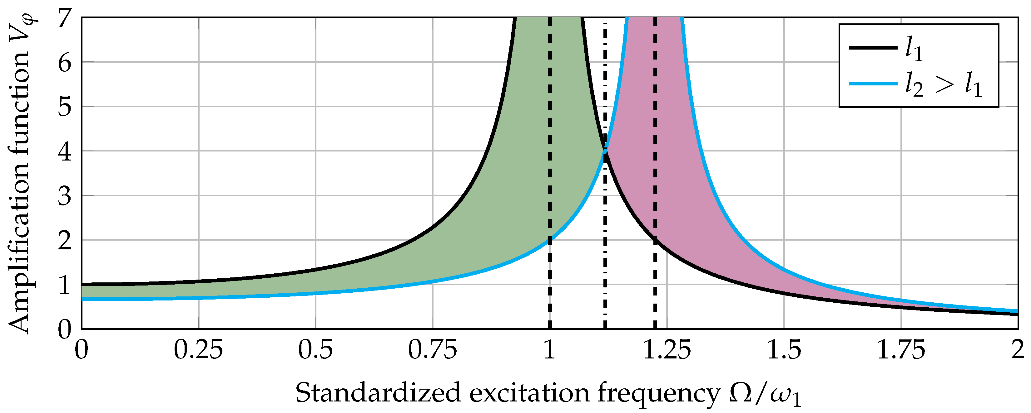
2.3. Validation of a Simplified Model
2.3.1. Knuckle
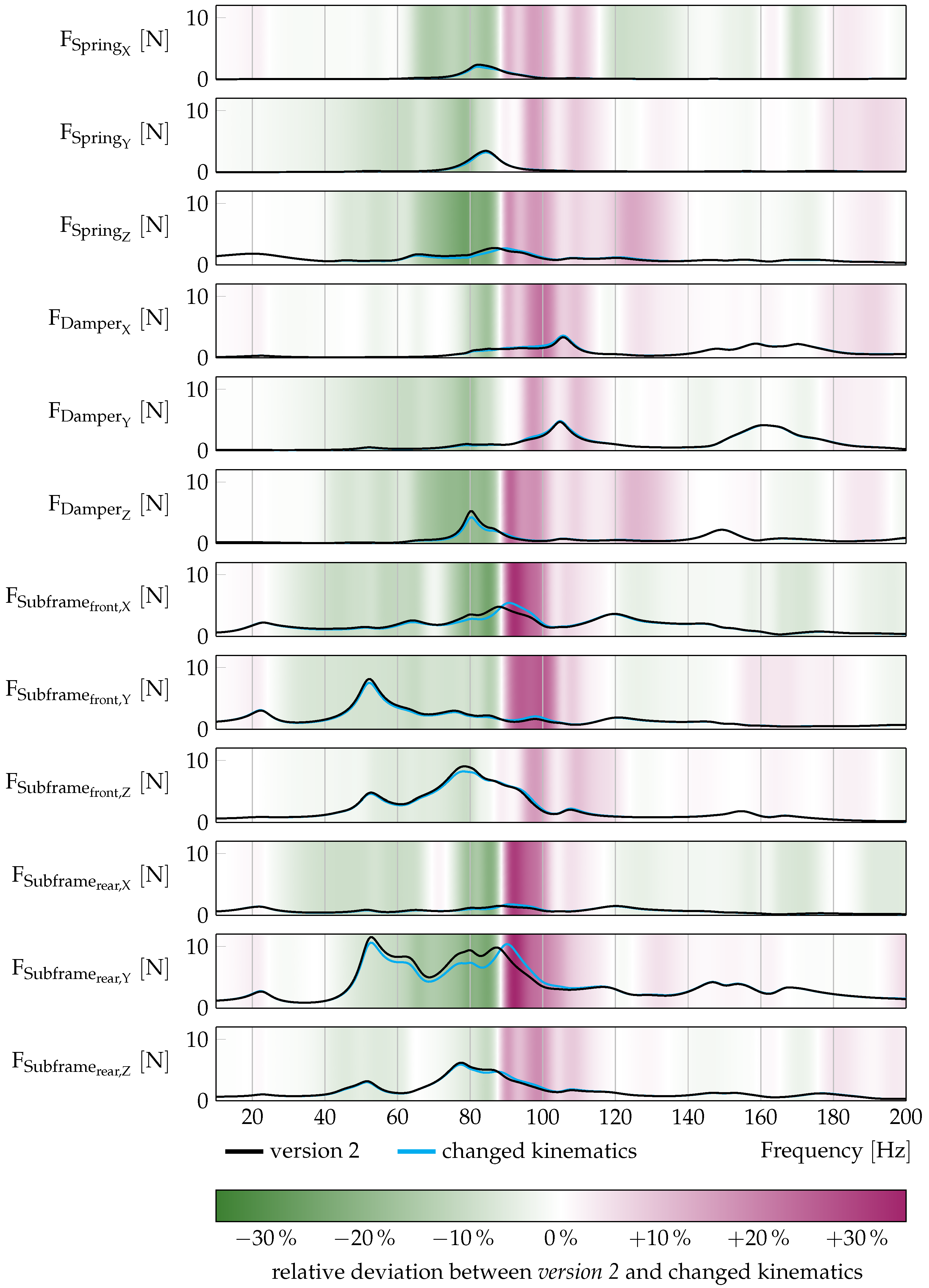
3. Results
4. Discussion
5. Conclusions
Author Contributions
Funding
Acknowledgments
Conflicts of Interest
Abbreviations
| ANC | Active Noise Cancelling |
| CAD | Computer Aided Design |
| FE | Finite Element |
| FRF | Frequency Response Function |
| MAC | Modal Assurance Criterion |
| MBS | Multi Body Simulation |
| NVH | Noise Vibration and Harshness |
| OEM | Original Equipment Manufacturer |
| RMS | Root Mean Square |
References
- Pfeffer, P.E. Die Komplexität kann man nicht reduzieren. ATZextra 2018, 23, 6–9. [Google Scholar] [CrossRef]
- Rambacher, C.; Ehrt, T.; Sell, H. Schwingungsoptimierung ganzer Achsen. Automob. Z. 2017, 119, 54–59. [Google Scholar] [CrossRef]
- Mantovani, M. Rollgeräusche kann man nicht mit Emotionen verbinden. Automob. Z. 2018, 120, 18–21. [Google Scholar] [CrossRef]
- Kim, J.K.; Lee, J.; Kim, H.G.; Cho, M.; Ih, K.D.; Ko, H.Y.; Shim, J.S. The Effects of Suspension Component Stiffness on the Road Noise: A Sensitivity Study and Optimization. In Proceedings of the 10th International Styrian Noise, Vibration & Harshness Congress, Graz, Austria, 20–22 June 2018; SAE Technical Paper Series; SAE International: Warrendale, PA, USA, 2018; pp. 1–7. [Google Scholar] [CrossRef]
- Ersoy, M.; Gies, S. (Eds.) Fahrwerkhandbuch: Grundlagen, Fahrdynamik, Komponenten, Systeme, Mechatronik, Perspektiven, 5th ed.; ATZ/MTZ-Fachbuch; Springer Vieweg: Wiesbaden, Germany, 2017. [Google Scholar] [CrossRef]
- Elbers, C.; Bäumer, B.; Siddiqui, S.; Albers, I. Entwicklung und Optimierung einer innovativen Verbundlenkerachse. Aachener Kolloquium für Fahrzeug- und Motorentechnik 2009, 18, 537–552. [Google Scholar]
- Botev, S. Digitale Gesamtfahrzeugabstimmung für Ride und Handling; Vol. 684, Fortschritt-Berichte VDI Reihe 12, Verkehrstechnik/Fahrzeugtechnik; VDI Verlag GmbH: Düsseldorf, Germany, 2008. [Google Scholar]
- Schilp, A.; Bathelt, H. NVH development strategies for suspensions—Challenges and chances by autonomous driving. In Proceedings of the Automotive Acoustics Conference; Siebenpfeiffer, W., Ed.; Springer Vieweg: Wiesbaden, Germany, 2017. [Google Scholar] [CrossRef]
- Zeller, P. (Ed.) Handbuch Fahrzeugakustik: Grundlagen, Auslegung, Berechnung, Versuch, 3rd ed.; ATZ/MTZ-Fachbuch; Springer Vieweg: Wiesbaden, Germany, 2018. [Google Scholar] [CrossRef]
- Schlecht, A. Minimierung der Schwingungsempfindlichkeit von Kraftfahrzeugvorderachsen. Ph.D. Thesis, Technische Universität München, München, Germany, 2012. [Google Scholar]
- Willenborg, D. Elastomer-Fahrwerkslager Simulativ Ausgelegt. Wie Beeinflusst Eine Geometrieänderung Die Federkonstante? Available online: https://automobilkonstruktion.industrie.de/fahrwerk/wie-beeinflusst-eine-geometrieaenderung-die-federkonstante/ (accessed on 8 August 2018).
- Kido, I.; Nakamura, A.; Hayashi, T.; Asai, M. Suspension Vibration Analysis for Road Noise Using Finite Element Model; SAE Technical Paper Series; SAE International: Warrendale, PA, USA, 1999. [Google Scholar] [CrossRef]
- Cytrynski, S.; Neerpasch, U.; Bellmann, R.; Danner, B. Das aktive Fahrwerk des neuen GLE von Mercedes-Benz. Automob. Z. 2018, 120, 42–45. [Google Scholar] [CrossRef]
- Gäbel, G.; Millitzer, J.; Atzrodt, H.; Herold, S.; Mohr, A. Development and Implementation of a Multi-Channel Active Control System for the Reduction of Road Induced Vehicle Interior Noise. Actuators 2018, 7, 52. [Google Scholar] [CrossRef]
- Zafeiropoulos, N.; Zollner, J.; Kandade Rajan, V. Aktive Dämpfung des Rollgeräuschs zur Verbesserung der Klangqualität im Fahrzeug. Automob. Z. 2018, 120, 38–43. [Google Scholar] [CrossRef]
- Schirle, T. Systementwurf eines elektromechanischen Fahrwerks für Megacitymobilität. Ph.D. Thesis, Karlsruher Institut für Technologie, Karlsruhe, Germany, 2019. [Google Scholar] [CrossRef]
- Troulis, M.; Gnadler, R.; Unrau, H.J. Übertragungsverhalten von Radaufhängungen für Personenwagen im komfortrelevanten Frequenzbereich. Automob. Z. 2004, 106, 336–348. [Google Scholar] [CrossRef]
- Chatillon, M.M.; Jezequel, L.; Coutant, P.; Baggio, P. Hierarchical optimization of the design parameters of a vehicle suspension system. Veh. Syst. Dyn. 2006, 44, 817–839. [Google Scholar] [CrossRef]
- Niersmann, A. Modellbasierte Fahrwerkauslegung und -Optimierung. Ph.D. Thesis, Technische Universität Braunschweig, Braunschweig, Germany, 2012. [Google Scholar]
- Vosteen, K. Ein Realtool zur Fahrwerkentwicklung. Aachener Kolloquium für Fahrzeug- und Motorentechnik 2008, 17, 1573–1591. [Google Scholar]
- Klein, B. FEM; Springer Fachmedien: Wiesbaden, Germany, 2015. [Google Scholar] [CrossRef]
- Fang, X.; Tan, K. Effiziente Konzeptauslegung von Verbundlenker-Hinterachsen. Automob. Z. 2015, 117, 42–47. [Google Scholar] [CrossRef]
- Helm, D.; Huf, A.; Zimmer, H.; Kondziella, R. Anforderungen in der Frühen Phase der Gesamtfahrzeugauslegung; VDI-Berichte 2169; VDI Verlag GmbH: Düsseldorf, Germany, 2012; pp. 21–40. [Google Scholar]
- Daimler Global Media. Mercedes-Benz C-Klasse T-Modell (S205) 2014, Raumlenker-Hinterachse: 14C577_03. Available online: https://media.daimler.com/marsMediaSite/de/instance/picture.xhtml?oid=7535355&ls=L3NlYXJjaHJlc3VsdC9zZWFyY2hyZXN1bHQueGh0bWw_c2VhcmNoU3RyaW5nPUQyMTIzMjkmc2VhcmNoSWQ9MiZzZWFyY2hUeXBlPWRldGFpbGVkJmJvcmRlcnM9dHJ1ZSZyZXN1bHRJbmZvVHlwZUlkPTE3MiZ2aWV3VHlwZT10aHVtYnMmc29ydERlZmluaXRpb249UFVCTElTSEVEX0FULTImdGh1bWJTY2FsZUluZGV4PTAmcm93Q291bnRzSW5kZXg9NQ!!&rs=0 (accessed on 28 August 2019).
- Van der Seijs, M.V.; de Klerk, D.; Rixen, D.J. General framework for transfer path analysis: History, theory and classification of techniques. Mech. Syst. Signal Process. 2016, 68-69, 217–244. [Google Scholar] [CrossRef]
- Zhu, J.J.; Khajepour, A.; Esmailzadeh, E.; Kasaiezadeh, A. Ride quality evaluation of a vehicle with a planar suspension system. Veh. Syst. Dyn. 2012, 50, 395–413. [Google Scholar] [CrossRef]
- Van der Linden, P.; van der Auweraer, H.; Wyckaert, K.; Hendricx, W. Noise and Vibration Transfer Path Analysis; Bus 2000; IMechE Conference Transactions; Professional Engineering for IMechE: Bury St Edmunds, UK, 2000; pp. 47–56. [Google Scholar]
- Sell, H. Geräuschpfadanalyse für Hochfrequenten Körperschall; Fortschritte der Akustik; Deutsche Gesellschaft für Akustik: Oldenburg, Germany, 2001. [Google Scholar]
- Rainieri, C.; Fabbrocino, G. Operational Modal Analysis of Civil Engineering Structures; Springer: New York, NY, USA, 2014. [Google Scholar] [CrossRef]
- Merziger, G.; Mühlbach, G.; Wille, D.; Wirth, T. Formeln + Hilfen höhere Mathematik, 8th ed.; Binomi-Verlag: Barsinghausen, Germany, 2018. [Google Scholar]
- Stevens, R. Discrete Sibson (Natural Neighbor) Interpolation: Naturalneighbor: 0.2.1. Available online: https://pypi.org/project/naturalneighbor/ (accessed on 19 August 2019).
- Open Source Initiative. The MIT License. Available online: https://opensource.org/licenses/MIT (accessed on 3 September 2019).
- Park, S.W.; Linsen, L.; Kreylos, O.; Owens, J.D.; Hamann, B. Discrete Sibson interpolation. IEEE Trans. Vis. Comput. Graph. 2006, 12, 243–253. [Google Scholar] [CrossRef] [PubMed]
- SciPy.org. Scipy.Interpolate.RegularGridInterpolator. Available online: https://docs.scipy.org/doc/scipy-0.16.1/reference/generated/scipy.interpolate.RegularGridInterpolator.html (accessed on 3 September 2019).


© 2020 by the authors. Licensee MDPI, Basel, Switzerland. This article is an open access article distributed under the terms and conditions of the Creative Commons Attribution (CC BY) license (http://creativecommons.org/licenses/by/4.0/).
Share and Cite
von Wysocki, T.; Chahkar, J.; Gauterin, F. Small Changes in Vehicle Suspension Layouts Could Reduce Interior Road Noise. Vehicles 2020, 2, 18-34. https://doi.org/10.3390/vehicles2010002
von Wysocki T, Chahkar J, Gauterin F. Small Changes in Vehicle Suspension Layouts Could Reduce Interior Road Noise. Vehicles. 2020; 2(1):18-34. https://doi.org/10.3390/vehicles2010002
Chicago/Turabian Stylevon Wysocki, Timo, Jason Chahkar, and Frank Gauterin. 2020. "Small Changes in Vehicle Suspension Layouts Could Reduce Interior Road Noise" Vehicles 2, no. 1: 18-34. https://doi.org/10.3390/vehicles2010002
APA Stylevon Wysocki, T., Chahkar, J., & Gauterin, F. (2020). Small Changes in Vehicle Suspension Layouts Could Reduce Interior Road Noise. Vehicles, 2(1), 18-34. https://doi.org/10.3390/vehicles2010002