A Recursive Wheel Wear and Vehicle Dynamic Performance Evolution Computational Model for Rail Vehicles with Tread Brakes


Abstract
:
1. Introduction
2. Materials and Methods
- Wear in the rail is much less as compared to that in the wheel and hence is not taken into account.
- The contact between wheel and rail is in dry condition and the presence of a third body (worn particles of wheel, rail and block, water, sand and leaves) is not considered.
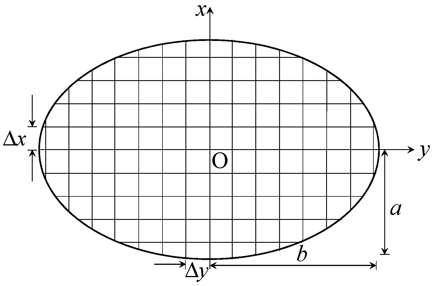
- The rail-wheel contact patch is elliptical in shape and the contact patch lies in the wheel tread, which is far away from the flange root.
- There is no wear in flange due to small duration, intermittent secondary contacts at entry and exit curves.
- The wheel and rail materials are same and have similar hardness.
- The wheel and rail material are isotropic, i.e., the material properties are same in all directions at a point but can vary from point to point due to change in temperature.
- The brake pad/shoe is made up of softer material (usually composite material with modulus of elasticity about ten times less as compared to wheel-rail material) and hence there is no wheel wear (but brake shoe/pad wear) at brake pad and wheel contact.
- The brake pads are assumed to be replaced periodically to maintain conformal contact between the brake pad and wheel tread, and the contact pressure between the wheel and brake pad is uniform.
- The heat partition between the wheel-rail-brake block is not influenced by the wheel wear.
- The influence of rail temperature variation is neglected in the model because it is usually much smaller than wheel temperature variation. Rail temperature is assumed to remain constant at 30 °C.
- Plastic deformation and fatigue effects are not considered.
- Spall formation, wheel flat etc. induced by phase transformation of the wheel and rail material at high contact pressure and temperature is neglected. The average contact patch pressure and temperature are considered for estimating the material properties while neglecting the local variations within the contact patch.
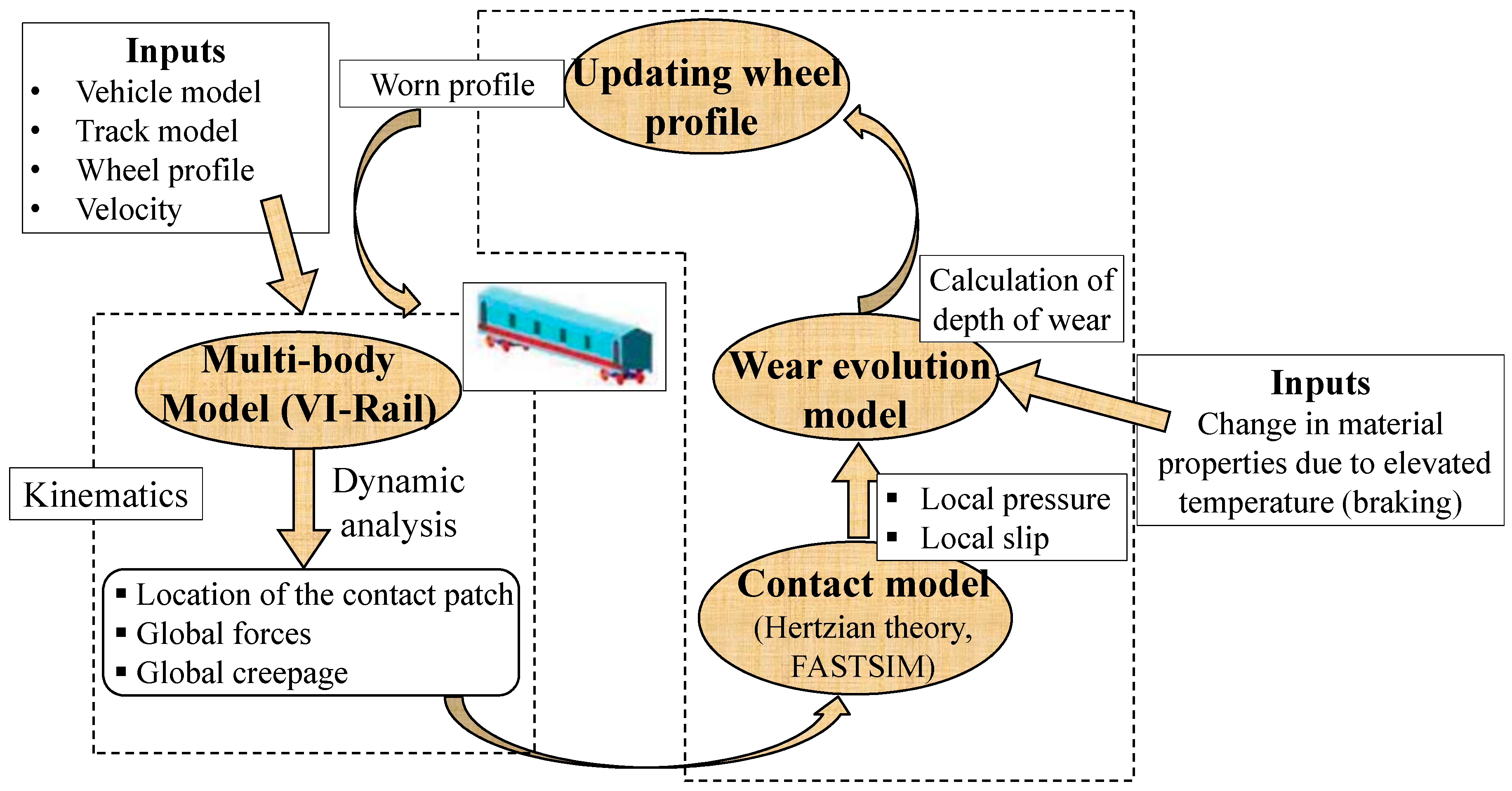
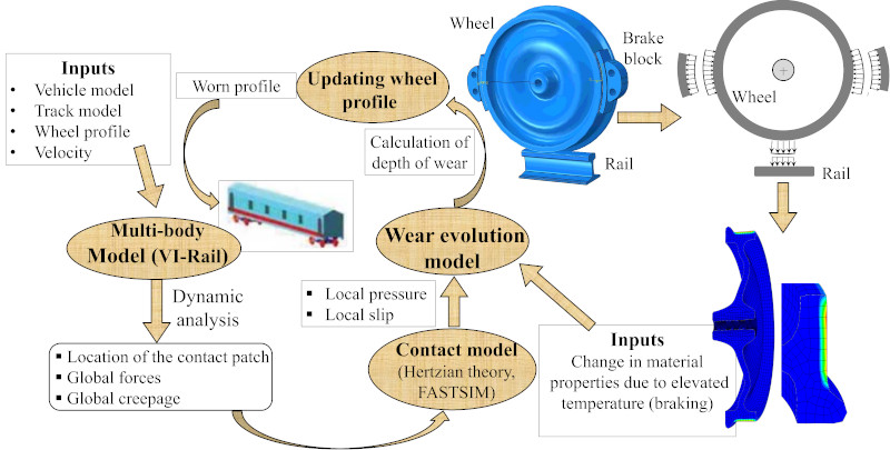
3. Wear Prediction Tool
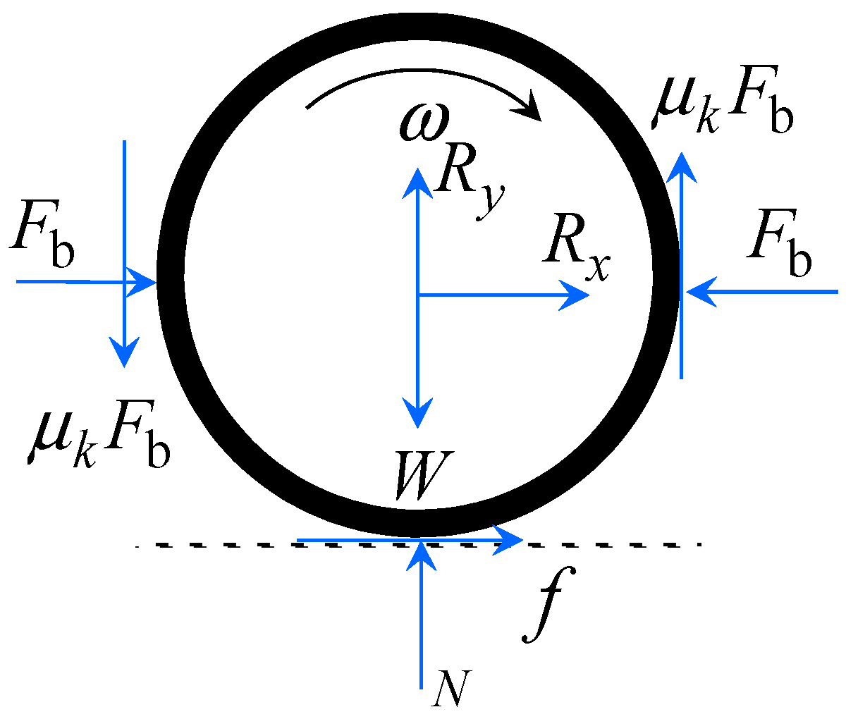
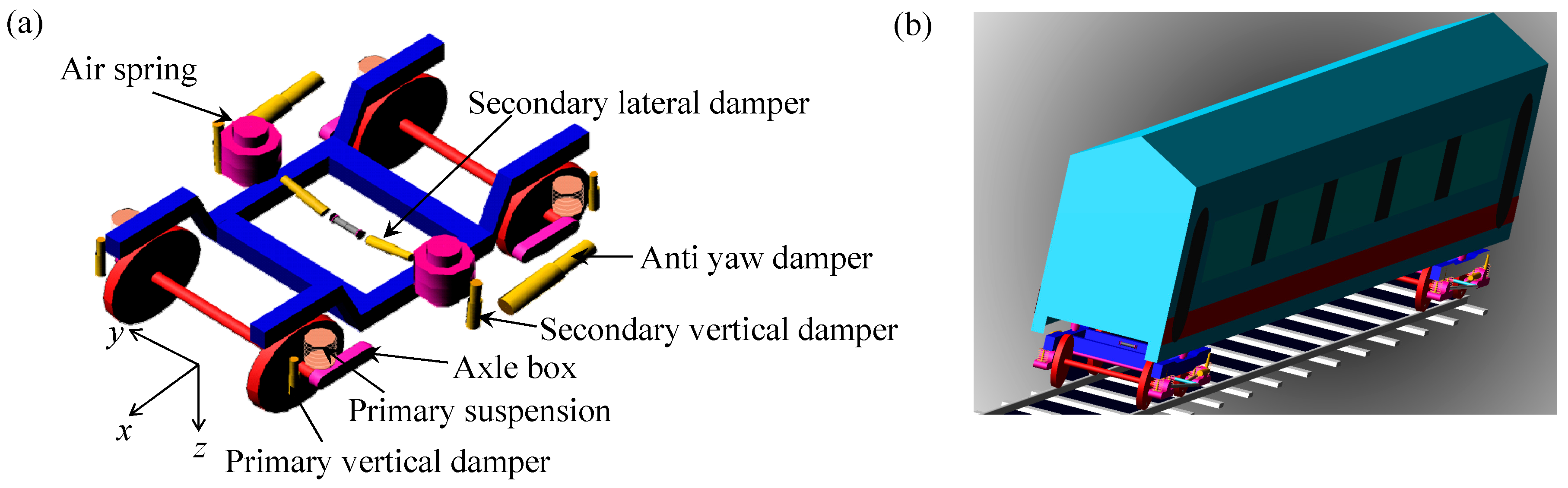
3.1. Vehicle Model
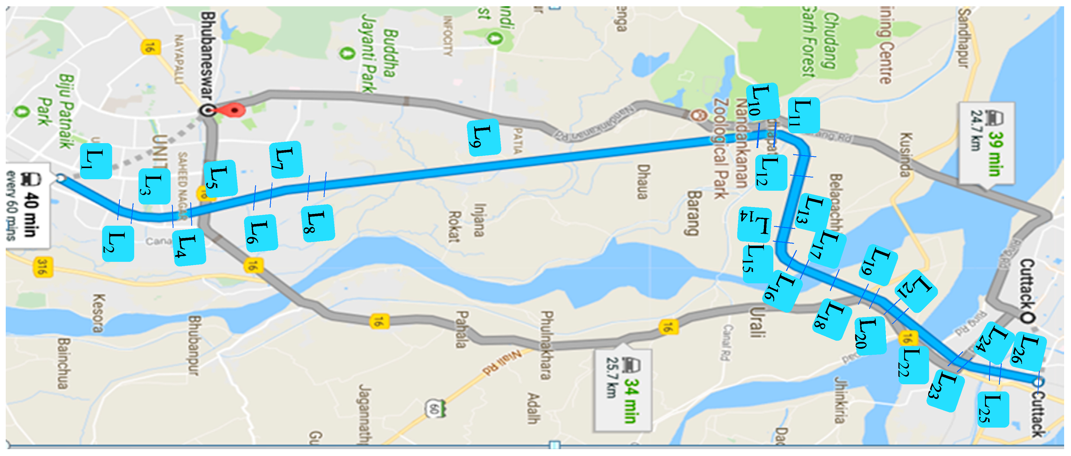
3.2. Track Model
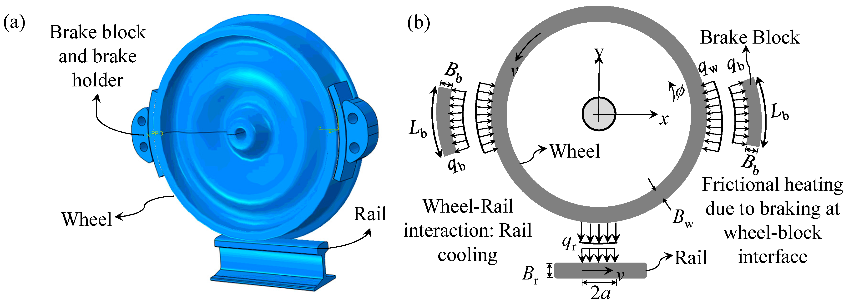
3.3. Thermal Model
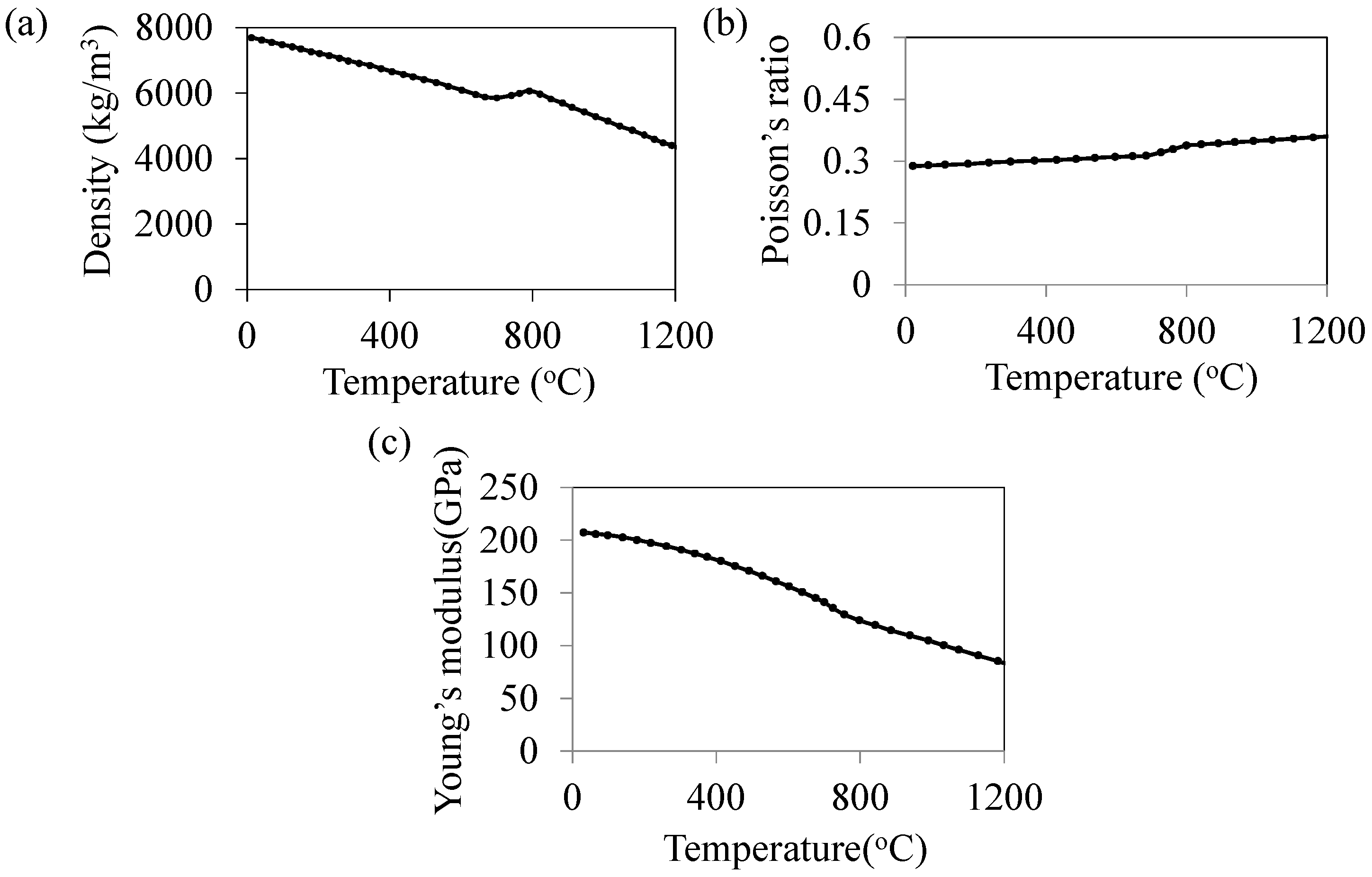
3.4. Material Properties
4. Wear Evolution Tool
4.1. Contact Model
4.2. Wear Model
4.3. Procedure for Updating Wheel Profile
5. Results
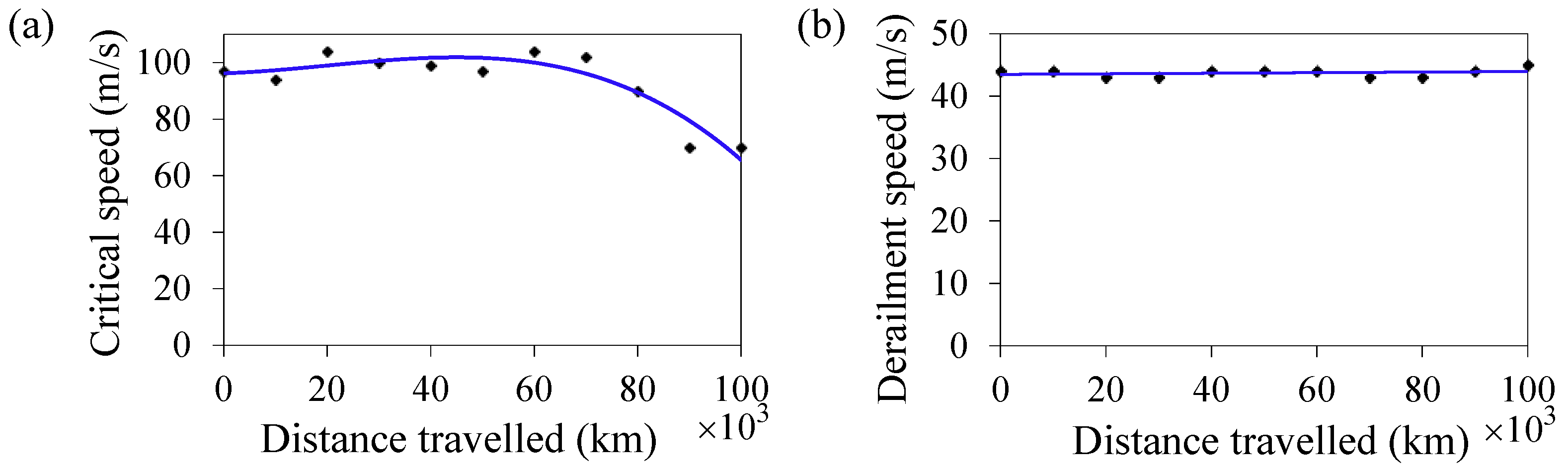
5.1. Stability Assessment
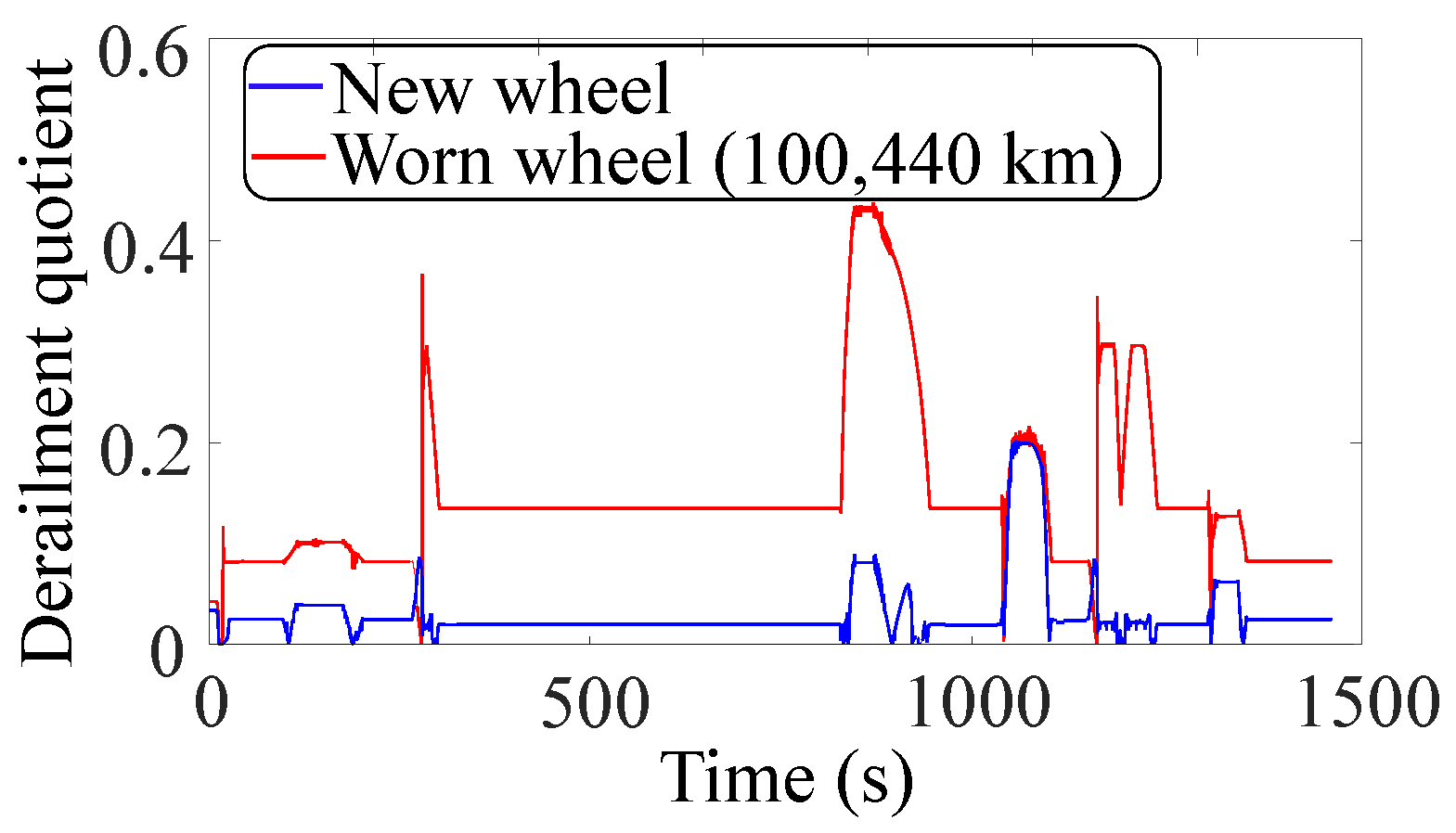
5.2. Derailment Quotient
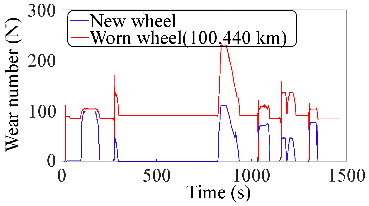
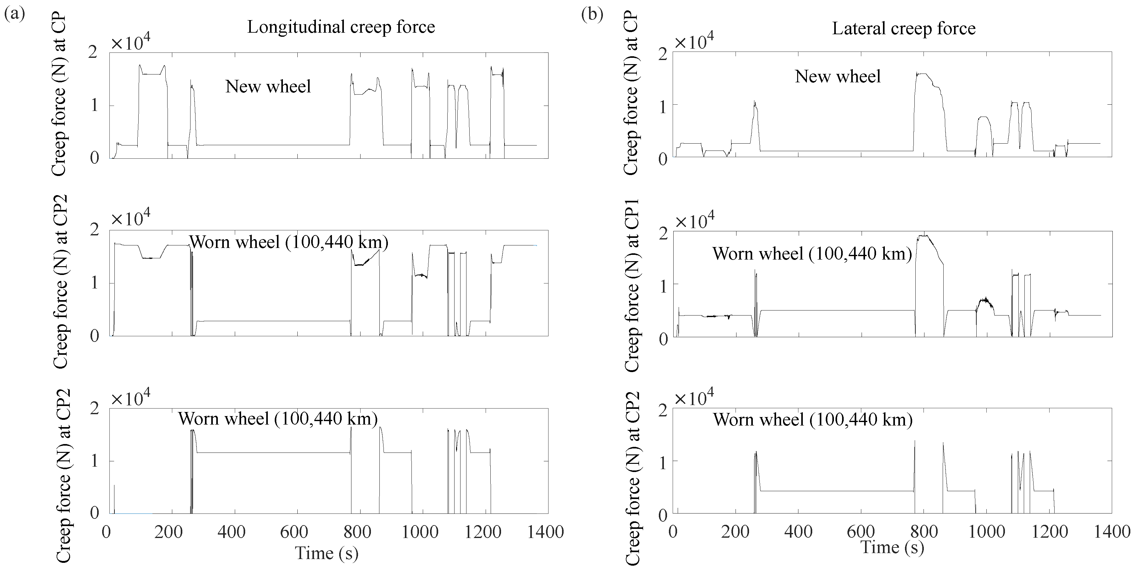
5.3. Wear Number
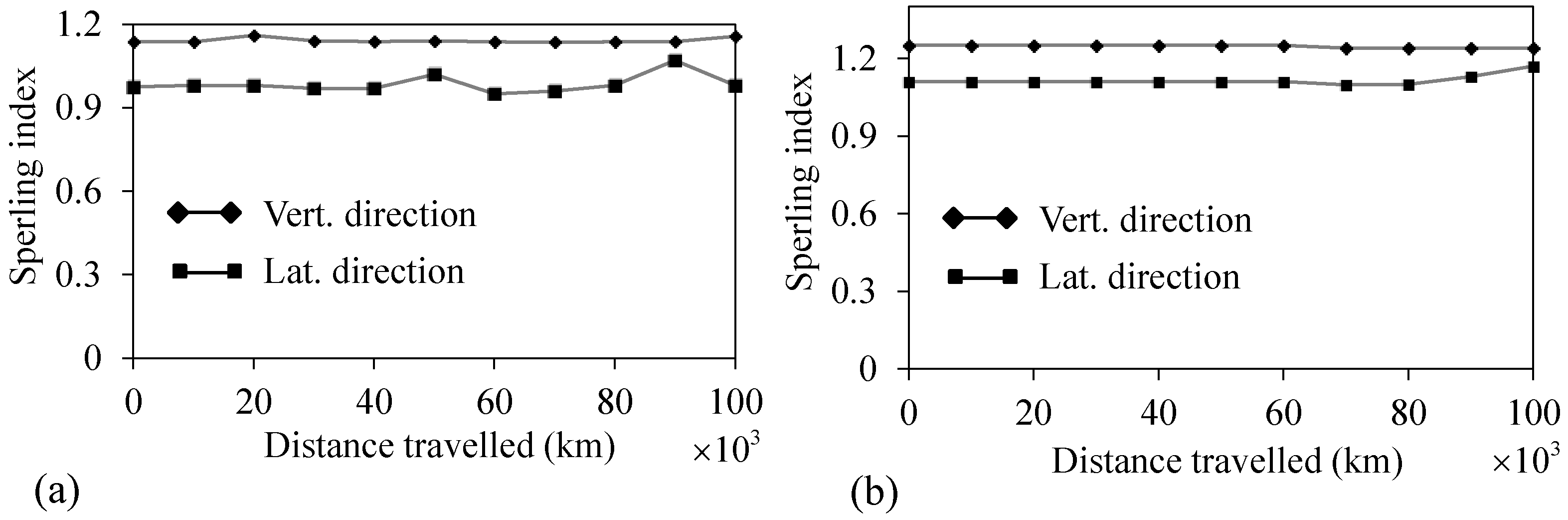
5.4. Passenger Comfort
6. Discussion
Author Contributions
Acknowledgments
Conflicts of Interest
Nomenclature
| Semi-major and semi-minor axes of the contact patch, respectively (mm). | |
| Ratio of friction coefficient () | |
| Coefficient of exponential friction decrease (s/m) | |
| Kalker’s parameters | |
| Specific heat capacity of the material (J/kg °C) | |
| Traction force at contact patch (N) /frequency of vibration | |
| Braking force (N). | |
| Longitudinal and lateral creep forces, respectively (N) | |
| Young’s modulus and Shear modulus (GPa). | |
| Brake block width (m) | |
| Thermal conductance (W/m2oC) | |
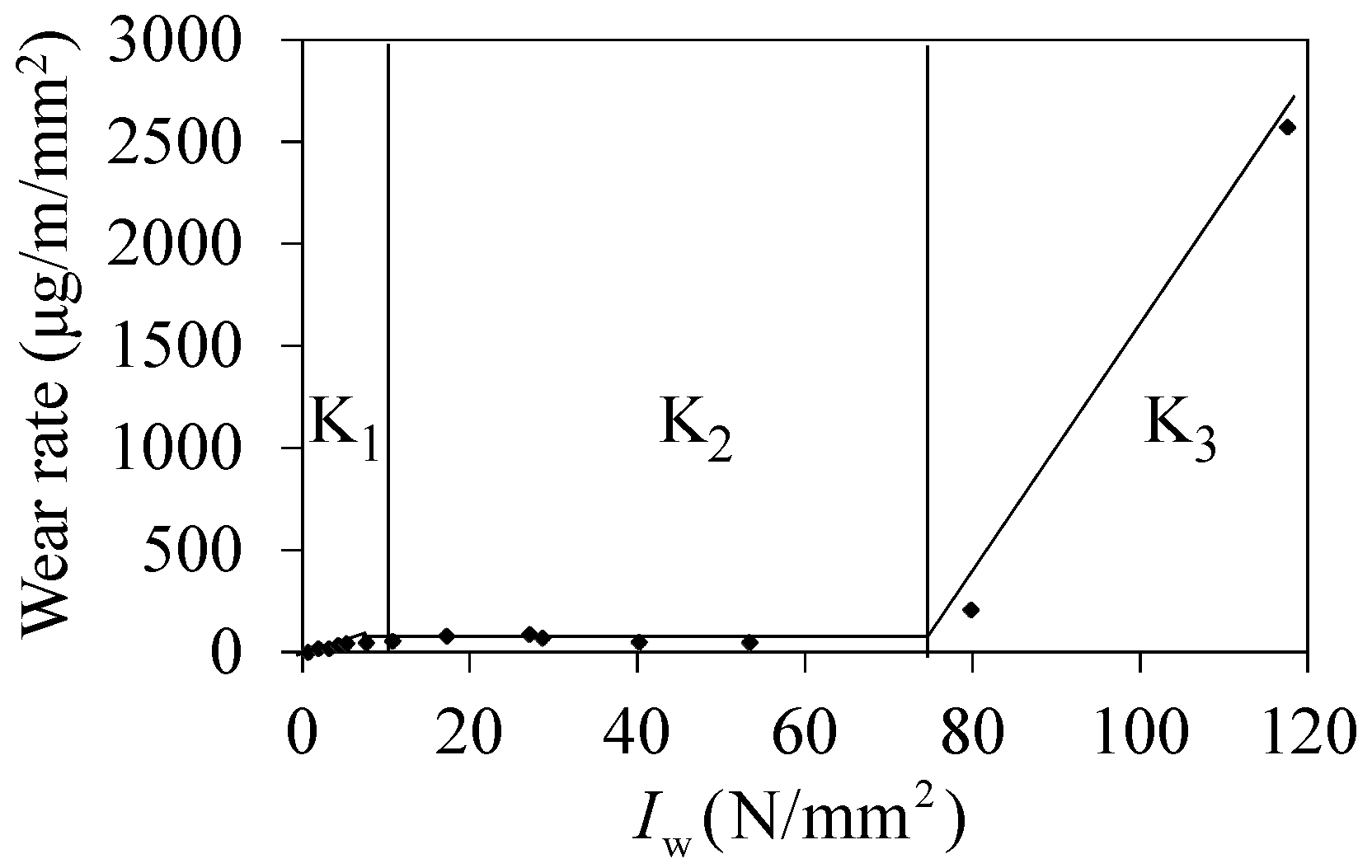
| Wear index (N/mm2) | |
| Polar moment of inertia of wheel and axle (N/m2) | |
| Thermal conductivity matrix | |
| Flexibility function | |
| Brake block length (m) | |
| Unit vector normal to the wheel surface | |
| Normal contact force (N) | |
| Total number of contact patches | |
| Numbers of cells in the contact patch in x and y directions, respectively. | |
| Adhesion limit pressure (N/m2) and tangential pressure (N/m2) | |
| Maximum pressure in the pressure distribution (N/m2) | |
| Mean heat flux over the brake block contact area (J/m2s) | |
| Amount of heat transfer through the convection (J/s) | |
| Mean radius of the wheel at nominal tread region (m) | |
| Reactions at axle in the x and y directions, respectively (N) | |
| Total slip (m/s) | |
| Time duration (s) | |
| Velocity vector of spatial points (m/s) | |
| Instantaneous temperature (°C) and ambient temperature (°C) | |
| Elastic displacement (m) | |
| Peripheral velocity of the wheel (m/s) | |
| Rigid slip (m/s) | |
| New and old wheel profiles | |
| Lateral and vertical forces, respectively (N) | |
| Heat transfer coefficient (W/Km2 or W/°Cm2) | |
| Global creepage vector | |
| Heat partition factor | |
| Thermal penetration depth (m) | |
| Specific volume of removed material | |
| Thermal diffusivity (m2/s) | |
| Thermal conductivity (W/m °C) | |
| Mass density (kg/m3) | |
| Angular velocity of the wheel (rad/s) | |
| Vector differential operator | |
| Coefficients of static and kinematic friction | |
| Maximum friction coefficient at zero slip and at infinity slip velocity | |
| , , | Longitudinal and lateral creepages (dimension-less), and spin creepage (m−1) |
| Poisson’s ratio |
References
- Laraqi, N. Velocity and relative contact size effects on the thermal constriction resistance in sliding solids. ASME J. Heat Transf. 1997, 119, 173–177. [Google Scholar] [CrossRef]
- Vernersson, T. Thermally induced roughness of tread braked railway wheels, Part 1: Brake rig experiments. Wear 1999, 236, 96–105. [Google Scholar] [CrossRef]
- Vernersson, T. Thermally induced roughness of tread braked railway wheels, Part 2: Modeling and field measurements. Wear 1999, 236, 106–116. [Google Scholar] [CrossRef]
- Godet, M. The third-body approach: A mechanical view of wear. Wear 1984, 100, 437–452. [Google Scholar] [CrossRef]
- Tanvir, M.A. Temperature rise due to slip between wheel and rail-an analytical solution for Hertzian contact. Wear 1980, 61, 295–308. [Google Scholar] [CrossRef]
- Knothe, K.; Liebelt, S. Determination of temperatures for sliding contact with applications for wheel-rail systems. Wear 1995, 189, 91–99. [Google Scholar] [CrossRef]
- Ertz, M.; Knothe, K. A comparison of analytical and numerical methods for the calculation of temperatures in wheel/rail contact. Wear 2002, 253, 498–508. [Google Scholar] [CrossRef]
- Ma, Y.; Markine, V.; Mashal, A.A.; Ren, M. Modelling verification and influence of operational patterns on tribological behaviour of wheel-rail interaction. Tribol. Int. 2017, 114, 264–281. [Google Scholar] [CrossRef]
- Tudor, A.; Radulescu, C.; Petre, I. Thermal effect of the brake shoes friction on the wheel/rail contact. Tribol. Ind. 2003, 25, 27–32. [Google Scholar]
- Spiryagin, M.; Lee, K.S.; Yoo, H.H.; Kashura, O.; Popov, S. Numerical calculation of temperature in the wheel–rail flange contact and implications for lubricant choice. Wear 2010, 268, 287–293. [Google Scholar] [CrossRef]
- Naeimi, M.; Li, S.; Li, Z.; Wu, J.; Petrov, R.H.; Sietsma, J.; Dollevoet, R. Thermomechanical analysis of the wheel-rail contact using a coupled modelling procedure. Tribol. Int. 2018, 117, 250–260. [Google Scholar] [CrossRef]
- Chen, W.W.; Wang, Q.J. Thermomechanical analysis of elastoplastic bodies in a sliding spherical contact and the effects of sliding speed, heat partition and thermal softening. J. Tribol. 2008, 130, 041402. [Google Scholar] [CrossRef]
- Kennedy, T.C.; Plengsaard, C.; Harder, R.F. Transient heat partition factor for a sliding railcar wheel. Wear 2006, 261, 932–936. [Google Scholar] [CrossRef]
- Teimourimanesh, S.; Vernersson, T.; Lunden, R. Thermal capacity of tread-braked railway wheels. Part 1: Modelling. J. Rail Rapid Transit 2016, 230, 784–797. [Google Scholar] [CrossRef]
- Teimourimanesh, S.; Vernersson, T.; Lunden, R. Thermal capacity of tread-braked railway wheels. Part 2: Application. J. Rail Rapid Transit 2016, 230, 798–812. [Google Scholar] [CrossRef]
- Ahlström, J.; Kabo, E.; Ekberg, A. Temperature-dependent evolution of cyclic stress of railway wheel steel. Wear 2016, 366, 378–382. [Google Scholar] [CrossRef]
- Cole, K.D.; Tarawneh, C.M.; Fuentes, A.A.; Wilson, B.M.; Navarro, L. Thermal models of railroad wheels and bearings. Int. J. Heat Mass Transf. 2010, 53, 1636–1645. [Google Scholar] [CrossRef]
- Peters, J.C.; Eifler, D. Influence of service temperatures on the fatigue behavior of railway wheel and tyre steels. Mater. Test. 2009, 51, 748–754. [Google Scholar] [CrossRef]
- Ahlström, J.; Karlsson, B. Microstructure evaluation and interpretation of the mechanically and thermally affected zone under railway wheel flat. Wear 1999, 232, 1–14. [Google Scholar] [CrossRef]
- Ahlström, J.; Karlsson, B. Analytical 1D model for analysis of the thermally affected zone formed during railway wheel skid. Wear 1999, 232, 15–24. [Google Scholar] [CrossRef]
- Asih, A.M.S.; Ding, K.; Kapoor, A. Modelling the effect of steady state wheel temperature on rail wear. Tribol. Lett. 2013, 49, 239–249. [Google Scholar] [CrossRef]
- Walia, M.S. Towards Enhanced Mechanical Braking Systems for Trains. Ph.D. Thesis, Chalmers University of Technology, Gothenburg, Sweden, 2017. [Google Scholar]
- Yang, Z.; Li, Z.; Dollevoet, R. Modelling of non-steady-state transition from single-point to two-point rolling contact. Tribol. Int. 2016, 101, 152–163. [Google Scholar] [CrossRef]
- Galas, R.; Kvarda, D.; Omasta, M.; Krupka, I.; Hartl, M. The role of constituents contained in water–based friction modifiers for top–of–rail application. Tribol. Int. 2018, 117, 87–97. [Google Scholar] [CrossRef]
- Archard, F. The temperature of rubbing surfaces. Wear 1959, 2, 438–455. [Google Scholar] [CrossRef]
- Pradhan, S.; Samantaray, A.K.; Bhattacharyya, R. Prediction of railway wheel wear and its influence on the vehicle dynamics in a specific operating sector of Indian railways network. Wear 2018, 406–407, 92–104. [Google Scholar] [CrossRef]
- Enblom, R.; Berg, M. Simulation of railway wheel profile development due to wear: Influence of disk braking and contact environment. Wear 2005, 258, 1055–1063. [Google Scholar] [CrossRef]
- Newcomb, T.P. Thermal aspects of railway braking. In Proceedings of the IMechE International Conference on Railway Braking, University of York, York, UK, 26–27 September 1979; pp. 7–18. [Google Scholar]
- Balakin, V.A.; Sergienko, V.P.; Komkov, O.Y. Heat transfer in friction contact zone at engagement of disc clutches and brakes. Sov. J. Frict. Wear 1997, 18, 450–455. [Google Scholar]
- Tian, X.; Kennedy, F.E., Jr. Maximum and average flash temperatures in sliding contacts. ASME J. Tribol. 1994, 116, 167–174. [Google Scholar] [CrossRef]
- Teimourimanesh, S.; Vernersson, T.; Lundén, R. Modeling of temperatures during railway tread braking: Influence of contact conditions and rail cooling effect. J. Rail Rapid Transit 2014, 228, 93–109. [Google Scholar] [CrossRef]
- Rafei, M.; Ghoreishy, M.H.R.; Naderi, G. Thermo-mechanical coupled finite element simulation of tire cornering characteristics—Effect of complex material models and friction law. Math. Comput. Simul. 2018, 144, 35–51. [Google Scholar] [CrossRef]
- Kragelski, I.V.; Dobycin, M.N.; Kombalov, V.S. Friction and Wear: Calculation Methods; Pergamon Press: Oxford, UK, 1982. [Google Scholar]
- Polach, O. Creep forces in simulations traction vehicles running on adhesion limit. Wear 2005, 258, 992–1000. [Google Scholar] [CrossRef]
- Dufrenoy, P. Etude du comportement thermomecanique des disques de freins vis a vis risques de defaillance ((Study of thermomechanical behavior of brake discs vis-à-vis risk of failure). Ph.D. Thesis, Universite des Science et Technologies de Lille, Cité Scientifique, France, 1995. [Google Scholar]
- Fischer, F.D.; Werner, E.; Knothe, K. The surface temperature of a half plane heated by friction and cooled by convection. Z. Angew. Math. Mech. 2001, 81, 75–81. [Google Scholar] [CrossRef]
- Baehr, H.D.; Stephan, K. Heat and Mass Transfer; Springer: Berlin, Germany, 1998. [Google Scholar]
- Kalker, J.J. Three-dimensional Elastic Bodies in Rolling Contact; Kluwer Academic Publishers: Dordrecht, The Netherlands, 1990. [Google Scholar]
- Dukkipati, R.V.; Amyot, J.R. Computer Aided Simulation in Railway Dynamics; Marcel Dekker: New York, NY, USA, 1988. [Google Scholar]
- Auciello, J.; Ignesti, M.; Malvezzi, M.; Meli, E.; Rindi, A. Development and validation of a wear model for the analysis of the wheel profile evolution in railway vehicles. Veh. Syst. Dyn. 2012, 50, 1707–1734. [Google Scholar] [CrossRef]
- Saunders, N.; Guo, U.K.Z.; Li, X.; Miodownik, A.P.; Schillé, J.P. Using JMatPro to model materials properties and behavior. J. Miner. Metals Mater. Soc. JOM 2003, 55, 60–65. [Google Scholar] [CrossRef]
- Pombo, J.; Ambrosio, J.; Pereira, M.; Lewis, R.; Dwyer-Joyce, R.; Ariaudo, C.; Kuka, N. Development of a wear prediction tool for steel railway wheels using three alternative wear functions. Wear 2011, 271, 238–245. [Google Scholar] [CrossRef]
- Braghin, F.; Lewis, R.; Dwyer-Joyce, R.S.; Bruni, S. A mathematical model to predict railway wheel profile evolution due to wear. Wear 2006, 261, 1253–1264. [Google Scholar] [CrossRef]
- Ignesti, M.; Marini, L.; Meli, E.; Rindi, A. Development of a model for the prediction of wheel and rail wear in the railway field. J. Comput. Nonlinear Dyn. 2012, 7, 041004. [Google Scholar] [CrossRef]
- Zhu, Y.; Olofsson, U.; Nilson, R. A field test study of leaf contamination on railhead surfaces. J. Rail Rapid Transit 2014, 228, 71–84. [Google Scholar] [CrossRef]
- Olofsson, U.; Zhu, Y.; Abbasi, S.; Lewis, R.; Lewis, S. Tribology of the wheel–rail contact–aspects of wear, particle emission and adhesion. Veh. Syst. Dyn. 2013, 51, 1091–1120. [Google Scholar] [CrossRef]
- Nikas, G.K. A mechanistic model of spherical particle entrapment in elliptical contacts. Proc. Ins. Mech. Eng. Part J J. Eng. Tribol. 2006, 220, 507–522. [Google Scholar] [CrossRef]
- Frischmuth, K.; Langemann, D. Numerical calculation of wear in mechanical systems. Math. Comput. Simul. 2011, 81, 2688–2701. [Google Scholar] [CrossRef]
- Esveld, C. Modern Railway Track, 2nd ed.; MRT-Productions: Delft, The Netherlands, 2001. [Google Scholar]
- Iwnicki, S. The Manchester Benchmarks for Rail Vehicle Simulators; Swets and Zeitlinger: Lisse, The Netherlands, 1999. [Google Scholar]
- Banerjee, N.; Karmakar, R. Modelling of a free rail wheel-set using non-linear creep force. Int. J. Heavy Veh. Syst. 2014, 21, 310–327. [Google Scholar] [CrossRef]
- Banerjee, N.; Karmakar, R. Bond graph modeling of rail wheel-set on curved track. Simulation 2007, 83, 695–706. [Google Scholar] [CrossRef]
- Banerjee, N.; Saha, A.K.; Karmakar, R.; Bhattacharyya, R. Bond graph modeling of a railway truck on curved track. Simul. Model. Pract. Theory 2009, 17, 22–34. [Google Scholar] [CrossRef]
- Polach, O.; Berg, M.; Iwnicki, S. Simulation. In Handbook of Railway Vehicle Dynamics; Iwnicki, S., Ed.; CRC Press: Boca Raton, FL, USA, 2006; pp. 359–421. [Google Scholar]
- Orlova, A.; Boronenko, Y. The anatomy of railway vehicle running gear. In Handbook of Railway Vehicle Dynamics; Iwnicki, S., Ed.; CRC Press: Boca Raton, FL, USA, 2006; pp. 39–83. [Google Scholar]
- Berthe, D.; Dowson, D.; Godet, M.; Taylor, C.M. (Eds.) Tribological Design of Machine Elements; Elsevier: Amsterdam, The Netherlands, 1989. [Google Scholar]
- Santamaría, J.; Vadillo, E.G.; Oyarzabal, O. Wheel–rail wear index prediction considering multiple contact patches. Wear 2009, 267, 1100–1104. [Google Scholar] [CrossRef]
- Hwang, I.K.; Hur, H.M.; Kim, M.J.; Park, T.W. Analysis of the active control of steering bogies for the dynamic characteristics on real track conditions. Proc. Ins. Mech. Eng. Part F J. Rail Rapid Transit 2018, 232, 722–733. [Google Scholar] [CrossRef]
- Garg, V.K.; Dukkipati, R.V. Dynamics of Railway Vehicle Systems; Academic Press: Cambridge, MA, USA, 1984. [Google Scholar]
- Samantaray, A.K.; Pradhan, S. Dynamic Analysis of Steering Bogies. In Handbook of Research on Emerging Innovations in Rail Transportation Engineering; Umesh Rai, B., Ed.; IGI Global: Hershey, PA, USA, 2016; pp. 524–579. [Google Scholar]
- Pradhan, S.; Samantaray, A.K. Integrated modeling and simulation of vehicle and human multi-body dynamics for comfort assessment in railway vehicles. J. Mech. Sci. Technol. 2018, 32, 109–119. [Google Scholar] [CrossRef]
- Nikas, G.K. Modeling dark and white layer formation on elastohydrodynamically lubricated steel surfaces by thermomechanical indentation or abrasion by metallic particles. J. Tribol. 2015, 137, 031504. [Google Scholar] [CrossRef]
- Li, X.; Yang, T.; Zhang, J.; Cao, Y.; Wen, Z.; Jin, X. Rail wear on the curve of a heavy haul line—Numerical simulations and comparison with field measurements. Wear 2016, 366, 131–138. [Google Scholar] [CrossRef]
- Ward, A.; Lewis, R.; Dwyer-Joyce, R.S. Incorporating a railway wheel wear model into multi-body simulations of wheelset dynamics. Tribol. Ser. 2003, 41, 367–376. [Google Scholar]
- Lewis, R.; Braghin, F.; Ward, A.; Bruni, S.; Dwyer-Joyce, R.S.; Bel Knani, K.; Bologna, P. Integrating Dynamics and Wear Modelling to Predict Railway Wheel Profile Evolution. In 6th International Conference on Contact Mechanics and Wear of Rail/Wheel Systems; Ekberg, A., Kabo, E., Ringsberg, J., Eds.; CHARMEC: Gothenburg, Sweden, 2003; pp. 7–16. [Google Scholar]
- Shevtsov, I.Y.; Markine, V.L.; Esveld, C. Optimal design of wheel profile for railway vehicles. Wear 2005, 258, 1022–1030. [Google Scholar] [CrossRef]
- Jahed, H.; Farshi, B.; Eshraghi, M.A.; Nasr, A. A numerical optimization technique for design of wheel profiles. Wear 2008, 264, 1–10. [Google Scholar] [CrossRef]
- Jo, H.J.; Kwak, S.W.; Yang, J.M. Vehicle Localization Using Internal Sensors and Low-Cost GPS for Autonomous Driving. J. Korean Inst. Intell. Syst. 2017, 27, 209–214. [Google Scholar] [CrossRef]


| Parameters of MBS Model | Parameter Values | Quantity |
|---|---|---|
| Mass of car body | MCB = 32,000 kg | 1 |
| Rotary inertias of car body | Ixx = 5.68 × 10⁴ kg m2 | |
| Iyy = 1.97 × 10⁶ kg m2 | ||
| Izz = 1.97 × 10⁶ kg m2 | ||
| Mass of Bogie frame | Mbogie = 2615 kg | 2 |
| Rotary inertias of bogie frame | Ixx = 1722 kg m2 | |
| Iyy = 1476 kg m2 | ||
| Izz = 3067 kg m2 | ||
| Mass of Wheel-set | Mwheel = 1503 kg | 4 |
| Rotary inertias of wheel-set | Ixx = 810 kg m2 | |
| Iyy = 810 kg m2 | ||
| Izz = 112 kg m2 | ||
| Mass of Axle-box | Mabox = 155 kg | 8 |
| Rotary inertias of axle box | Ixx= 2.1 kg m2 | |
| Iyy= 5.6 kg m2 | ||
| Izz= 5.6 kg m2 | ||
| Stiffness of Primary suspension | Kx = 6.8 × 10⁶ N/m | 8 |
| Ky = 3.92 × 10⁶ N/m | ||
| Kz = 5.756 × 10⁵ N/m | ||
| Kθ = Kα = 63.5 Nm/rad | ||
| Nominal pressure of Secondary suspension (Air spring) | Pstatic = 2.0532 × 10⁵ Pa | 4 |
| Primary vertical damper (series stiffness) | 1.0 × 10⁶ N/m | 8 |
| Secondary vertical damper (series stiffness) | 6.0 × 10⁶ N/m | 4 |
| Secondary anti-yaw damper (series stiffness) | 3.0 × 10⁷ N/m | 4 |
| Secondary lateral damping (series stiffness) | 6.0 × 10⁶ N/m | 4 |
© 2019 by the authors. Licensee MDPI, Basel, Switzerland. This article is an open access article distributed under the terms and conditions of the Creative Commons Attribution (CC BY) license (http://creativecommons.org/licenses/by/4.0/).
Share and Cite
Pradhan, S.; Samantaray, A.K. A Recursive Wheel Wear and Vehicle Dynamic Performance Evolution Computational Model for Rail Vehicles with Tread Brakes. Vehicles 2019, 1, 88-115. https://doi.org/10.3390/vehicles1010006
Pradhan S, Samantaray AK. A Recursive Wheel Wear and Vehicle Dynamic Performance Evolution Computational Model for Rail Vehicles with Tread Brakes. Vehicles. 2019; 1(1):88-115. https://doi.org/10.3390/vehicles1010006
Chicago/Turabian StylePradhan, Smitirupa, and Arun Kumar Samantaray. 2019. "A Recursive Wheel Wear and Vehicle Dynamic Performance Evolution Computational Model for Rail Vehicles with Tread Brakes" Vehicles 1, no. 1: 88-115. https://doi.org/10.3390/vehicles1010006
APA StylePradhan, S., & Samantaray, A. K. (2019). A Recursive Wheel Wear and Vehicle Dynamic Performance Evolution Computational Model for Rail Vehicles with Tread Brakes. Vehicles, 1(1), 88-115. https://doi.org/10.3390/vehicles1010006