Closed-Form Solution of a Special Case of a Vehicle Longitudinal Motion Model

Abstract

One of the most common approaches in modern engineering research, including vehicle dynamics, is to formulate an accurate, but typically complex, mathematical model of a system or phenomenon and then use a software package to solve it. Typically, the solution is obtained in the form of a large data set, which may be difficult to analyse and interpret. This paper represents a purely theoretical analysis of a special case of vehicle longitudinal motion. Starting from a simplified mathematical model, a set of transcendental equations was derived that represents the exact solution of the model (i.e., in a closed form). The equations are analysed and interpreted in terms of what is their physical meaning. Although the equations derived here have only limited application in studying real world problems, due to the simplicity of the mathematical model, they offer a deeper insight into the nature of vehicle longitudinal motion.

1. Introduction

Vehicle dynamics, including vehicle longitudinal motion, is a well-researched area and there are numerous very accurate mathematical models that describe various aspects of vehicle motion. Supported by a continuous increase in computing power, there is a distinctive trend towards more complex models that include more phenomena, resulting in high-fidelity models, which do not have closed-form solutions. Due to the complexity, approximate solutions are normally obtained via numerical methods, usually using some engineering software packages, such as Matlab.

This is a well-accepted approach in engineering and the solutions can be very accurate. However, such solutions are never exact, and they are normally given in the form of large data sets, which makes it difficult to analyse them. Having an exact solution is always preferred, not only because there is a qualitative difference between an approximate and the exact solution, but also because closed-form solutions are easily analysed and offer greater insights into the nature of the motion.

With this in mind, we looked into the most common models from the area of vehicle dynamics in order to find out those that require only minor simplifications so that their solutions can be found in a closed form. We found model (1) as a prime example where relatively small simplifications allow the direct integration of the differential equations, leading to an interesting set of equations that describes vehicle longitudinal motion.

After an extensive research of the literature, it was found that no such attempt had been carried out. It appears that this idea has been overlooked, and in that way we missed an opportunity to better understand some aspects of vehicle dynamics.

In an attempt to calculate rolling resistance coefficient and vehicle aerodynamic coefficient, White and Korst [1] partially solved model (1) in a closed form while setting traction force and climbing resistance to zero. Obviously, such a solution is very different from the solution obtained in this paper. A similar approach was used in [2], which takes into account climbing resistance and models rolling resistance as a function of velocity squared F_f = F_f (v²).

The inception and evolution of vehicle dynamics and associated mathematical models, as well as anticipated future developments, are presented in [3], whereas [4] presents diverse views and practices in the verification and validation of vehicle dynamics simulation models. A comprehensive review of numerical methods used in vehicle system dynamics is presented in [5].

Lugner and Plochl in [6] provide a top-level overview and classification of the mathematical models currently used in vehicle dynamics. They note that simplifications allow the decoupling of the lateral, longitudinal, and vertical dynamics, and creation of models that describe each respective motion separately from the other two. Such models allow partially analytical derivations of corresponding equations of motion, which, according to them, is useful for studying how input parameters influence the motion. This view is aligned with the aims of this paper. However, in the section dedicated to longitudinal dynamics, they focus on other aspects of longitudinal motion and stop short from deriving the equations presented here.

One approach to modelling vehicle longitudinal motion is presented in [7], although the focus of the paper is on the control design. Another approach is shown in [8], where air drag and tyre rolling resistance are ignored for simplicity, while focusing on the stability of longitudinal and lateral motion.

Typically, equations of the motion of a multi-body system are obtained either via the Newton–Euler or via the Lagrange approach. For instance, the Lagrange approach was used in [9] to create a vehicle model with ten degrees of freedom, which was then used to study the Anti-Lock Brake System (ABS).

Vehicle longitudinal dynamics have multiple aspects and different models are used to capture them. For instance, there is a complex interaction between the tyre and the road (which is critical for both longitudinal and lateral dynamics), relative motion of the car body with respect to the wheels, engine, transmission, and brake characteristics, etc. To capture the nature of the longitudinal motion at the highest level, model (1) and the closed-form solution presented in this paper seem most suitable.

This paper is organised as follows: Section 2 describes the mathematical model studied in this paper. Section 3 is the core of the paper where closed-form solutions are derived, followed by Section 4 with the analysis and interpretation of the results. Section 5 provides a brief conclusion and a summary.

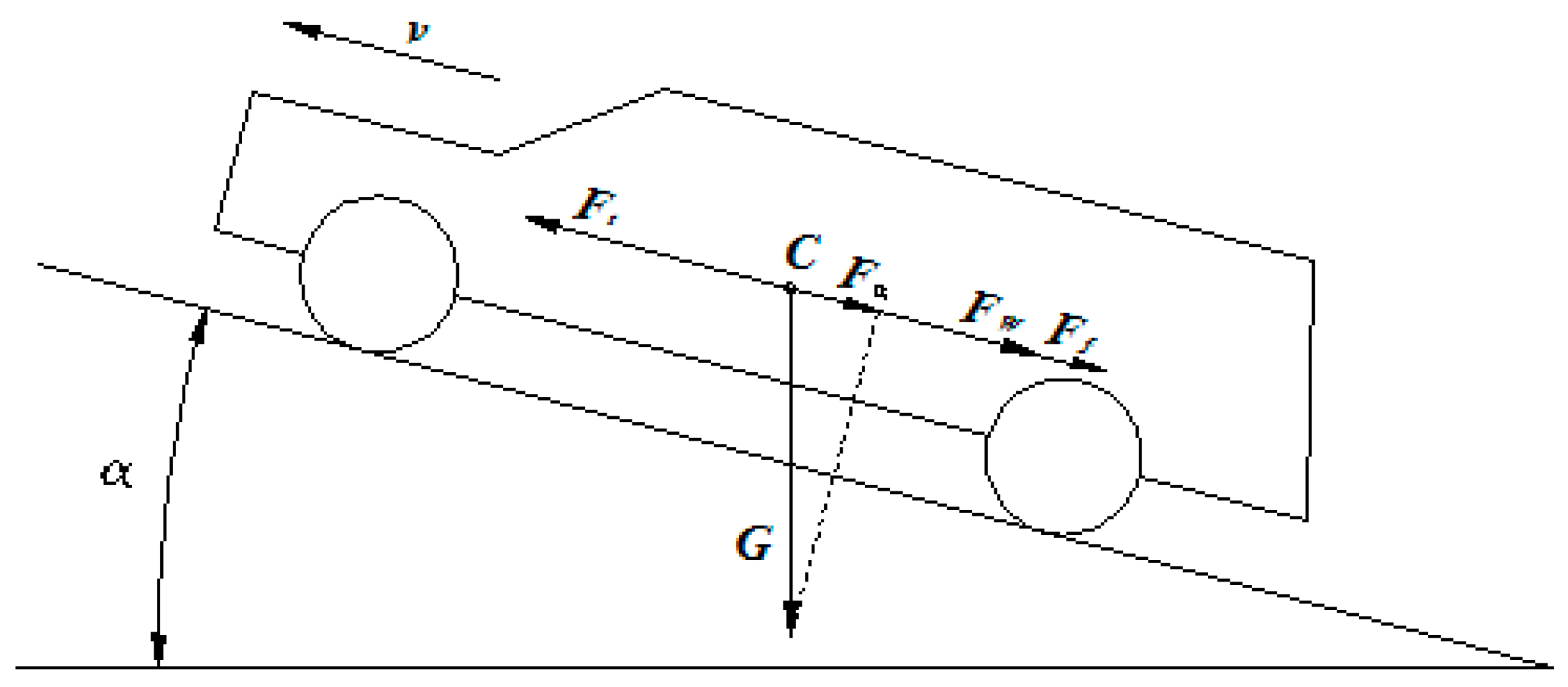
2. Model Description

This paper is focused on a special case of vehicle longitudinal motion governed by the following four forces, as shown in Figure 1:

• Total traction force F_t;
• Total rolling resistance F_f;
• Climbing resistance F_α;
• Air drag resistance F_W.

Model details and assumptions:

• Vehicle is considered a rigid body, with one degree of freedom. The only coordinate required to identify its position is distance travelled (s);
• Vehicle moves through still air, in a straight line, on an even road surface with a constant gradient;
• For simplicity, and because of linear motion, all vectors are treated as scalars. Forces are positive if they act in the same direction as the vehicle velocity. If they act in the opposite direction, their values are negative. The same applies to acceleration;
• Total traction force Ft, total rolling resistance F_f, and climbing resistance F_α are all constant forces, whereas air drag resistance F_W is a function of the vehicle speed.

According to Newton’s second law of motion, the product of a body’s mass and acceleration is equal to the sum of all forces acting on that body. In the case of a vehicle moving in a straight line, this leads to a well-known equation of motion:

$$m\cdot \frac{dv}{dt}={\displaystyle \sum _i{F}_i}=F_f+F_{\alpha }+F_t+F_W$$

(1)

It needs to be mentioned here that it is not uncommon in the literature to denote the left side of (1) as acceleration resistance or inertial resistance [10]. We suggest that it is better to avoid such terminology as some readers could confuse this “resistance” with real force acting on the vehicle, which it is not. The inertial force of a body (vehicle) is equal to the negative product of the body’s mass and acceleration. This force does not act upon the body, it acts on the matter that causes a change of the body’s velocity, and in the case of a vehicle, that matter is the surrounding air and road.

In engineering studies, for velocities typical for road traffic, rolling resistance value is usually modelled according to (2) and assumed to be constant. Even if this force is modelled as a function of velocity squared, as it is done in [2], the solution of model (1) could still be found in a closed form.

$$F_f=G\cdot f$$

(2)

Climbing resistance is given by (3) and, for a constant gradient, it is a constant force. The force is negative when driving uphill, whereas driving downhill creates a positive force.

$$F_{\alpha }=G\cdot \sin (\alpha )$$

(3)

Traction force is created when an internal moment is applied to any of the wheels. If brakes are activated, then such a moment creates negative traction force, whereas a propulsive moment on driving wheels creates positive force. In real world situations, this force varies continuously during driving, but in this model it is assumed to be constant.

Air drag resistance is a function of vehicle speed, and it is usually modelled as per (4). It is always negative as it acts in the opposite direction to vehicle velocity.

$$F_W=C_W\cdot A\cdot \frac{\rho \cdot v^2}{2}$$

(4)

Models (2)–(4) are well accepted in the literature. For instance, they were used and explained in more detail in [10] and [11].

3. Model Solution

Equation (1) is an ordinary nonlinear differential equation of the second order (considering that velocity is a first-order derivation of distance). Solving Equation (1) means finding velocity and travelled distance as functions of time: v = v(t), s = s(t), which, in the general case, is not possible. Due to the variability of traction force, it is not possible to use integrals to obtain solutions of (1) in a closed form (exact solutions). However, if one assumes constant traction force, then integrals can be used to obtain exact solutions of (1), as shown in (5). This assumption is not far from reality if the motion is studied in segments (piecewise), especially when driving outside of urban areas.

$$m\cdot {\displaystyle \underset{}{\overset{}{\int }}\frac{dv}{\left(F_f+F_{\alpha }+F_t\right)-C_W\cdot A\cdot \frac{\rho \cdot v^2}{2}}}={\displaystyle \underset{}{\overset{}{\int }}dt}$$

(5)

To simplify Equation (5), let us introduce the following constants:

$$K_1=C_W\cdot A\cdot \frac{\rho }{2}$$

(6)

$$K_2=F_f+F_{\alpha }+F_t$$

(7)

$$K_3{}^2=\frac{K_2}{K_1}$$

(8)

At this point, the solution branches into two paths, depending on the sign of the sum of forces K₂. Given that K₁ is always positive and (8), it follows that K₂ also has to be positive. If the resulting force in Equation (7) is greater than zero (positive), then coefficient K₂ is defined by (7) and marked as K₂+. This leads to a set of equations describing a particular type of motion. Otherwise, if the resulting force in Equation (7) is negative, then coefficient K₂ is defined by (25) and marked as K₂-. This leads to a set of equations describing a different type of motion.

3.1. Case When K₂ > 0

Using (6)–(8), Equation (5) can be transformed into:

$$m\cdot {\displaystyle \underset{}{\overset{}{\int }}\frac{dv}{K_2^{+}-K_1\cdot v^2}}=\frac{m}{K_1}\cdot {\displaystyle \underset{}{\overset{}{\int }}\frac{dv}{K_3{}^2-v^2}}={\displaystyle \int dt}$$

(9)

After integrating (9), one can obtain:

$$K_4\cdot \ln \left|\frac{v-K_3}{v+K_3}\right|=t+C$$

(10)

where:

$$K_4=-\frac{m}{K_1}\cdot \frac{1}{2\cdot K_3}$$

(11)

Equation (10) is equivalent to the following:

$$\left|\frac{v-K_3}{v+K_3}\right|=e^{\frac{t+C_{}}{K_4}}$$

(12)

We are now experiencing the second bifurcation point because there are two solutions to (12): one for the case when v > K₃ and the second for the case when v < K₃. Let us explore them.

3.1.1. Case When v > K₃

When v > K₃, Equation (12) is equivalent to:

$$\frac{v-K_3}{v+K_3}=e^{\frac{t+C_1}{K_4}}$$

(13)

from which one can obtain the final expression for velocity as a function of time:

$$v^{v>K_3}(t)=K_3\frac{1+e^{\frac{t+C_1}{K_4}}}{1-e^{\frac{t+C_1}{K_4}}}$$

(14)

The constant of integration C₁ can be obtained from the initial conditions for velocity and (13):

$$\begin{array}{l}t=t_1\\ v=v_1\end{array}|\Rightarrow C_1=K_4\cdot \ln \frac{v_1-K_3}{v_1+K_3}-t_1$$

(15)

To find distance travelled as a function of time s = s(t), we need to integrate the expression for velocity (14), leading to:

$${\displaystyle \int ds}=K_3\cdot {\displaystyle \int \frac{1+e^{\frac{t+C_1}{K_4}}}{1-e^{\frac{t+C_1}{K_4}}}dt}+C_2$$

(16)

The solution can be expressed as:

$$s^{v>K_3}(t)=K_3\cdot K_4\cdot \ln \frac{\left|e^{\frac{t+C_1}{K_4}}\right|}{{\left(e^{\frac{t+C_1}{K_4}}-1\right)}^2}+C_2$$

(17)

The constant of integration C₂ can be obtained from the initial conditions for distance travelled:

$$\begin{array}{l}t=t_1\\ s=s_1\end{array}|\Rightarrow C_2=s_1-K_3\cdot K_4\cdot \ln \frac{\left|e^{\frac{t_1+C_1}{K_4}}\right|}{{\left(e^{\frac{t_1+C_1}{K_4}}-1\right)}^2}$$

(18)

3.1.2. Case When v < K₃

When v < K₃, Equation (12) is equivalent to:

$$\frac{v-K_3}{v+K_3}=-e^{\frac{t+C_3}{K_4}}$$

(19)

from which one can obtain the final expression for velocity as a function of time:

$$v^{v<K_3}(t)=K_3\frac{1-e^{\frac{t+C_3}{K_4}}}{1+e^{\frac{t+C_3}{K_4}}}$$

(20)

The constant of integration C₃ can be obtained from the initial conditions for velocity and (19):

$$\begin{array}{l}t=t_1\\ v=v_1\end{array}|\Rightarrow C_3=K_4\cdot \ln \frac{K_3-v_1}{v_1+K_3}-t_1$$

(21)

Integrating the expression for velocity (20), one can find distance as a function of time s = s(t):

$${\displaystyle \int ds}=K_3\cdot {\displaystyle \int \frac{1-e^{\frac{t+C_3}{K_4}}}{1+e^{\frac{t+C_3}{K_4}}}dt}+C_4$$

(22)

The solution can be expressed as:

$$s^{v<K_3}(t)=K_3\cdot K_4\cdot \ln \frac{\left|e^{\frac{t+C_3}{K_4}}\right|}{{\left(e^{\frac{t+C_3}{K_4}}+1\right)}^2}+C_4$$

(23)

with the constant of integration:

$$\begin{array}{l}t=t_1\\ s=s_1\end{array}|\Rightarrow C_4=s_1-K_3\cdot K_4\cdot \ln \frac{\left|e^{\frac{t_1+C_3}{K_4}}\right|}{{\left(e^{\frac{t_1+C_3}{K_4}}+1\right)}^2}$$

(24)

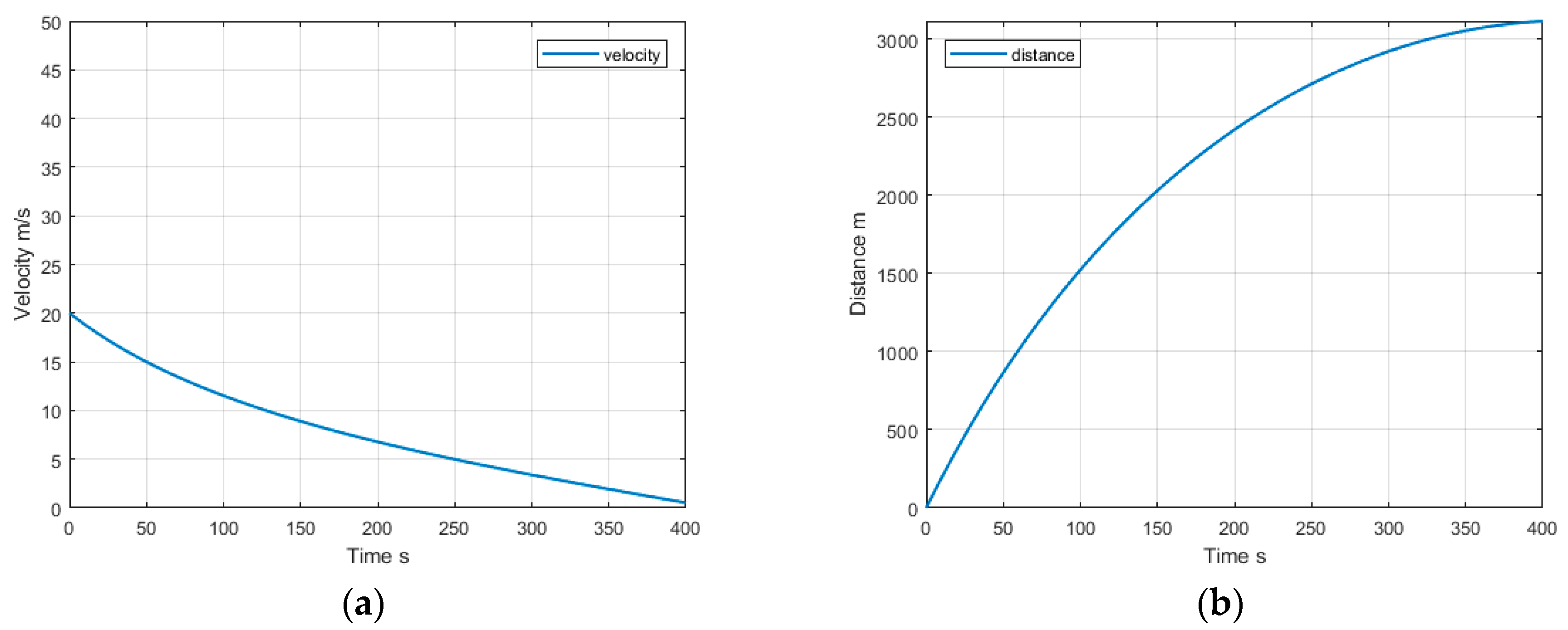
3.2. Case When K₂ < 0

In this case, the sum of the three forces (F_f, F_α, F_t) is negative, whereas, as mentioned earlier, K₂ has to be always positive to satisfy (8). To accommodate for that, K₂ will have to be redefined as follows, and marked as K₂-:

$$K_2^{-}=-\left(F_f+F_{\alpha }+F_t\right)$$

(25)

Starting from Equation (5) and redefined coefficient K₂ (25), one can get:

$$m\cdot {\displaystyle \underset{}{\overset{}{\int }}\frac{dv}{-K_2^{-}-K_1\cdot v^2}}=-\frac{m}{K_1}\cdot {\displaystyle \underset{}{\overset{}{\int }}\frac{dv}{K_3{}^2+v^2}}={\displaystyle \int dt}$$

(26)

Integration of (26) yields:

$$\frac{-m}{K_1}\cdot \frac{1}{K_3}\cdot arctg\left(\frac{v}{K_3}\right)=t+C_5$$

(27)

Constant C₅ can be obtained from the initial conditions:

$$\begin{array}{l}t=t_1\\ v=v_1\end{array}|\Rightarrow C_5=\frac{-m}{K_1\cdot K_3}arctg\frac{v_1}{K_3}-t_1$$

(28)

The final expression for velocity as a function of time can be derived from (27):

$$v(t)=K_3\tan \left[\frac{-\left(t+C_5\right)\cdot K_1\cdot K_3}{m}\right]$$

(29)

To obtain the expression for distance travelled, one needs to integrate the expression for velocity (29):

$${\displaystyle \underset{}{\overset{}{\int }}ds}=K_3{\displaystyle \underset{{}_{}}{\overset{}{\int }}\tan \left[K_5\cdot t+K_5\cdot C_5\right]}dt+C_6$$

(30)

where:

$$K_5=-\frac{K_1\cdot K_3}{m},$$

(31)

Solving (30) yields the final expression for distance travelled as a function of time:

$$s(t)=-\frac{K_3}{K_5}\ln \left|\cos \left(K_{5}t+K_5\cdot C_5\right)\right|+C_6$$

(32)

with the constant of integration C₆ determined by:

$$\begin{array}{l}t=t_1\\ s=s_1\end{array}|\Rightarrow C_6=s_1+\frac{K_3}{K_5}\ln \left|\cos \left(K_5{t}_1+K_5\cdot C_5\right)\right|$$

(33)

In the next section, these equations will be analysed to understand how they can be interpreted and what their physical meaning is.

4. Analysis of the Results

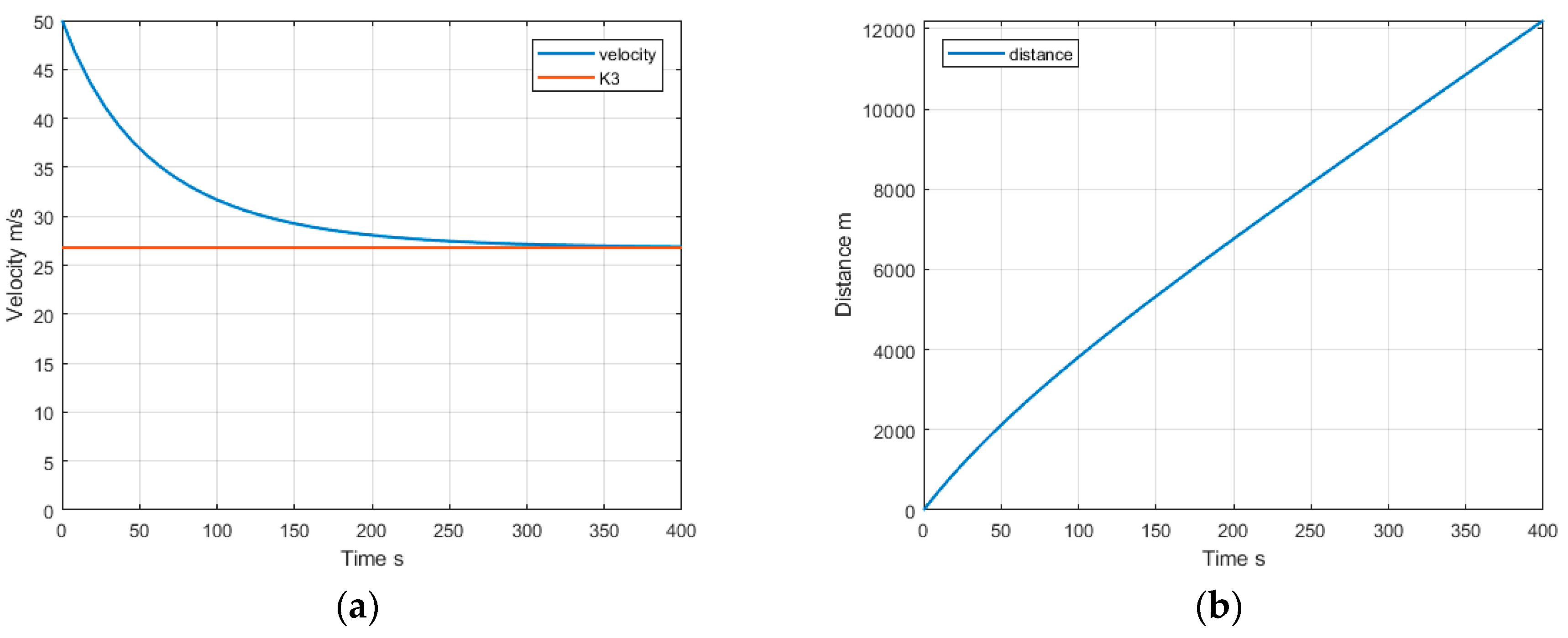
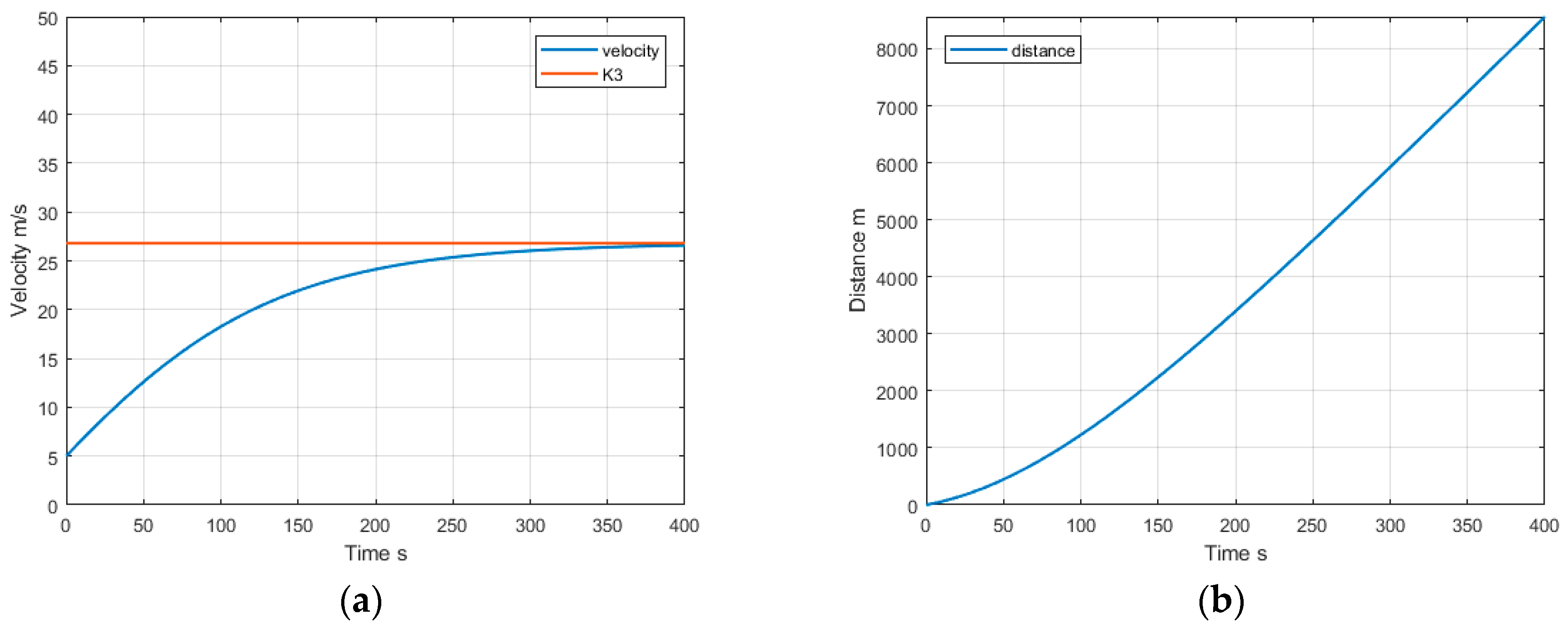
4.1. Case When K₂ > 0

We have seen how the relation between initial velocity and coefficient K₃ determines the type of motion and the governing equations. Considering that both v and K₃ have to be nonnegative, let us investigate what is the physical meaning of v < K₃ and v > K₃.

4.1.1. Case When v > K₃

It can be shown that:

$$v>K_3\iff F_f+F_{\alpha }+F_t+F_W<0$$

(34)

or

$$v>K_3\iff F_f+F_{\alpha }+F_t<-F_W$$

(35)

which means that the resulting force acting on the vehicle is negative. The direct consequence is that acceleration is negative and velocity decreases. Using only logical reasoning, one can infer:

• If the sum of three forces (K₂ = F_f + F_α + F_t) is positive but the vehicle decelerates, the absolute value of air resistance F_W, which is greater than the sum according to (35), will also decrease;
• At some point, the absolute value of F_W will become equal to the sum of the other three forces, when deceleration stops and velocity reaches a constant value;
• It takes infinite time to reach this point.

Let us prove these inferences and find the velocity minimum. We can use the right-hand side of (13) and, keeping in mind that K₄ is always negative, find:

$$\underset{t\to \infty }{\lim }{e}^{\frac{t+C_1}{K_4}}=0^{+}\Rightarrow v\to K_3{}^{+}$$

(36)

where “0⁺” indicates an approach from the right-hand side. In other words, the vehicle will decelerate until velocity reaches the value of K₃. This type of motion is shown in Figure 2, where the red line represents the value of K₃. Specific values used to produce Figure 2, Figure 3 and Figure 4 are given in the Appendix A. The values are characteristic of a typical passenger car driving on a sealed road, under typical atmospheric conditions, but other values could be used as well, resulting in similar patterns.

4.1.2. Case When v < K₃

Conversely, it can be shown that v < K₃ means that the total resulting force is positive and the vehicle accelerates.

$$v<K_3\iff F_f+F_{\alpha }+F_t+F_W>0$$

(37)

In a similar fashion, one can conclude that the vehicle will continue to accelerate until the absolute value of F_W becomes equal to the sum of the other three forces, at which point velocity reaches the value of K₃. Again, it would take infinite time to reach this steady state motion. This type of motion is shown in Figure 3, and the red line again represents the value of K₃.

In terms of the stability of such motion (both v < K₃ and v > K₃ cases), any small disturbance that does not cause velocity to “cross the red line” (value of K₃) would not change the type of motion. If the vehicle is “pushed” to cross the value of K₃ (whether by accelerating or decelerating) then the type of motion would change, i.e., from v < K₃ type to v > K₃ type, or vice versa.

4.2. Case When K₂ < 0

Velocity in this case always decreases monotonically. A typical case of such motion is shown in Figure 4. To find out time to full stop, one can use (27) and put v = 0. As the function arctan returns zero value for zero argument, it follows that time to full stop is equal to:

$$t^{stop}=-C_5$$

(38)

Maximal distance travelled can be obtained from (32) simply by substituting time to stop (38) for time, resulting in:

$$s^{stop}=C_6$$

(39)

The specific case of motion shown in Figure 4 is characterised by the following parameters: C₅ = −419 s and C₆ = 3122 m, which can be obtained from (28) and (33), respectively, and using the values given in the Appendix A. Any small disturbance can not change this type of motion.

5. Conclusions

This paper presents a top-level analysis of vehicle longitudinal motion, and it identifies the necessary assumptions/simplifications in order to obtain a model that has a closed-form solution. The mathematical model studied here is quite simple and may not be suitable for practical engineering studies, for which there are numerous very accurate mathematical models and software packages that can solve them. However, the main contributions of this paper are:

• It derives a new set of equations that represent the exact solution (closed-form solution) of the mathematical model, describing a special case of vehicle longitudinal motion;
• It analyses the equations and reveals how relations between the four acting forces and initial velocity determine the nature of the longitudinal motion.

This paper does not propose the return to the pen-and-paper era or to forgo computer simulations. It just emphasises that closed-form solutions are more valuable than approximate (numerical) ones, and therefore they should be sought wherever possible.

References

1. White, R.A.; Korst, H.H. The Determination of Vehicle Drag Contributions from Coast down Tests. SAE Trans. 1972, 81, 354–359. [Google Scholar] [CrossRef]
2. Roussillon, G. Contribution to accurate measurement of aerodynamic drag on a moving vehicle from coast–down tests and determination of actual rolling resistance. J. Wind Eng. Ind. Aerodyn. 1981, 9, 33–48. [Google Scholar] [CrossRef]
3. Vantsevich, V.V. Road and off-road vehicle system dynamics. Understanding the future from the past. Veh. Syst. Dyn. 2015, 53, 137–153. [Google Scholar] [CrossRef]
4. Kutluay, E.; Winner, H. Validation of vehicle dynamics simulation models—A review. Veh. Syst. Dyn. 2014, 52, 186–200. [Google Scholar] [CrossRef]
5. Arnold, M.; Burgermeister, B.; Führer, C.; Hippmann, G.; Rill, G. Numerical methods in vehicle system dynamics: State of the art and current developments. Veh. Syst. Dyn. 2011, 49, 1159–1207. [Google Scholar] [CrossRef]
6. Lugner, P.; Plochl, M. Modelling in vehicle dynamics of automobiles. J. Appl. Math. Mech. 2004, 84, 219–236. [Google Scholar] [CrossRef]
7. Majdoub, K.E.; Giri, F.; Ouadi, H.; Dugard, L.; Chaoui, F.Z. Vehicle longitudinal motion modelling for nonlinear control. Contr. Eng. Pract. 2011, 20, 69–81. [Google Scholar] [CrossRef]
8. Chen, K.; Pei, X.; Ma, G.; Guo, X. Longitudinal/Lateral Stability Analysis of Vehicle Motion in the Nonlinear Region. Math. Prob. Eng. 2016, 2016, 3419108. [Google Scholar] [CrossRef]
9. Blagojevic, M. A Research of Possibilities of Realising of Motor Vehicle Braking without Blocking the Wheels. Magistar Thesis, University of Banja Luka, Banja Luka, Bosnia and Herzegovina, 2004. [Google Scholar]
10. Meywerk, M. Vehicle Dynamics; John Wiley & Sons Incorporated: New York, NY, USA, 2015. [Google Scholar]
11. Rajamani, R. Vehicle Dynamics and Control; Springer Science Business Media Inc.: New York, NY, USA, 2006. [Google Scholar]
Figure 1. Forces acting on the vehicle.
Vehicles 01 00007 g001
Figure 2. Parameters when K2 > 0 and v > K3, (a) Velocity and (b) Distance.
Vehicles 01 00007 g002
Figure 3. Parameters when K2 > 0 and v < K3, (a) Velocity and (b) Distance.
Vehicles 01 00007 g003
Figure 4. Parameters when K2 < 0, (a) Velocity and (b) Distance.
Vehicles 01 00007 g004