Abstract
In hybrid electric vehicles, energy management systems (EMS) using optimization show superior fuel efficiency compared to rule-based strategies. However, little research shows its real-life applicability. In Part II of this work, the multi-level, model-predictive EMS from Part I is implemented on a heavy-duty parallel hybrid electric vehicle, using GPS and map data as preview. The power split, hybrid mode, and gear selection, including switching costs, are optimized in real time, thereby proving the feasibility of optimal control techniques for hybrid driveline control. Functional validation of the EMS on a test track confirm the fuel-saving mechanism as simulated in Part I. In addition to a fuel saving of 36%, the EMS also improves the drivability, by reducing the amount of open driveline events.
1. Introduction
The Energy Management System (EMS) in a hybrid electric vehicle controls the energy flow in the drive train, for the best fuel efficiency and drivability. The state of the art in industry uses rule-based algorithms, as they can be easily calculated with the onboard computational power, but little information about the used algorithms is disclosed. An improved fuel efficiency is obtained with optimization-based algorithms, as simulation results show in [1,2,3,4,5,6,7,8,9]. As a next step towards real-life implementation, these algorithms are tested with hardware-in-the-loop [10,11] or with a complete vehicle on a roller dyno [12] and, finally, on the road [13]. Computational complexity of the optimization algorithm increases, if, besides continuous decision variables (power split, [10,11,12]), discrete decision variables (gear selection [13], stop-start) are also optimized.
This work contributes to the actual implementation and validation of the multi-level EMS [14], using preview, on a heavy-duty parallel hybrid electric truck. The EMS optimizes power split with four hybrid modes (including stop-start) and gear selection, taking into account switching costs and battery constraints. We thereby show that optimal control can be used to control the complete hybrid driveline.
To solve the mixed integer, multi-state optimal control problem, the EMS is partitioned in three functional levels, each with their own abstraction of the vehicle, calculating control information for the levels below [14]. On the lowest level, the power split, mode, and gear shifting are optimized; on the middle level, the battery energy is optimized; and on the top level, the power demand is predicted. On a test track with elevation changes, validation is performed, and demonstrated for each level separately, to give insight in the accuracy and the effects on the system performance. Using GPS, map data, and the vehicle state for preview, the model-predictive EMS is solved in real time, providing high fuel efficiency and drivability, while the amount of tuning is minimal due to the model-based approach.
In Section 2, the vehicle characteristics, the test conditions, and the architecture of the implemented strategy are described. The functional validation of the EMS is explained in three parts: the prediction of the power demand in Section 3; the battery energy control in Section 4; and the control of the power split, mode, and gear in Section 5.
2. Vehicle, Test Setup, and Implementation
To validate the behavior and performance of the EMS with preview on the road, measurements are performed on a test track with elevation changes, with a DAF XF 105 heavy-duty hybrid electric vehicle. In this section, the vehicle (Section 2.1), the test track (Section 2.2) and implementation details of the EMS (Section 2.3) are described.
2.1. Hybrid Electric Vehicle
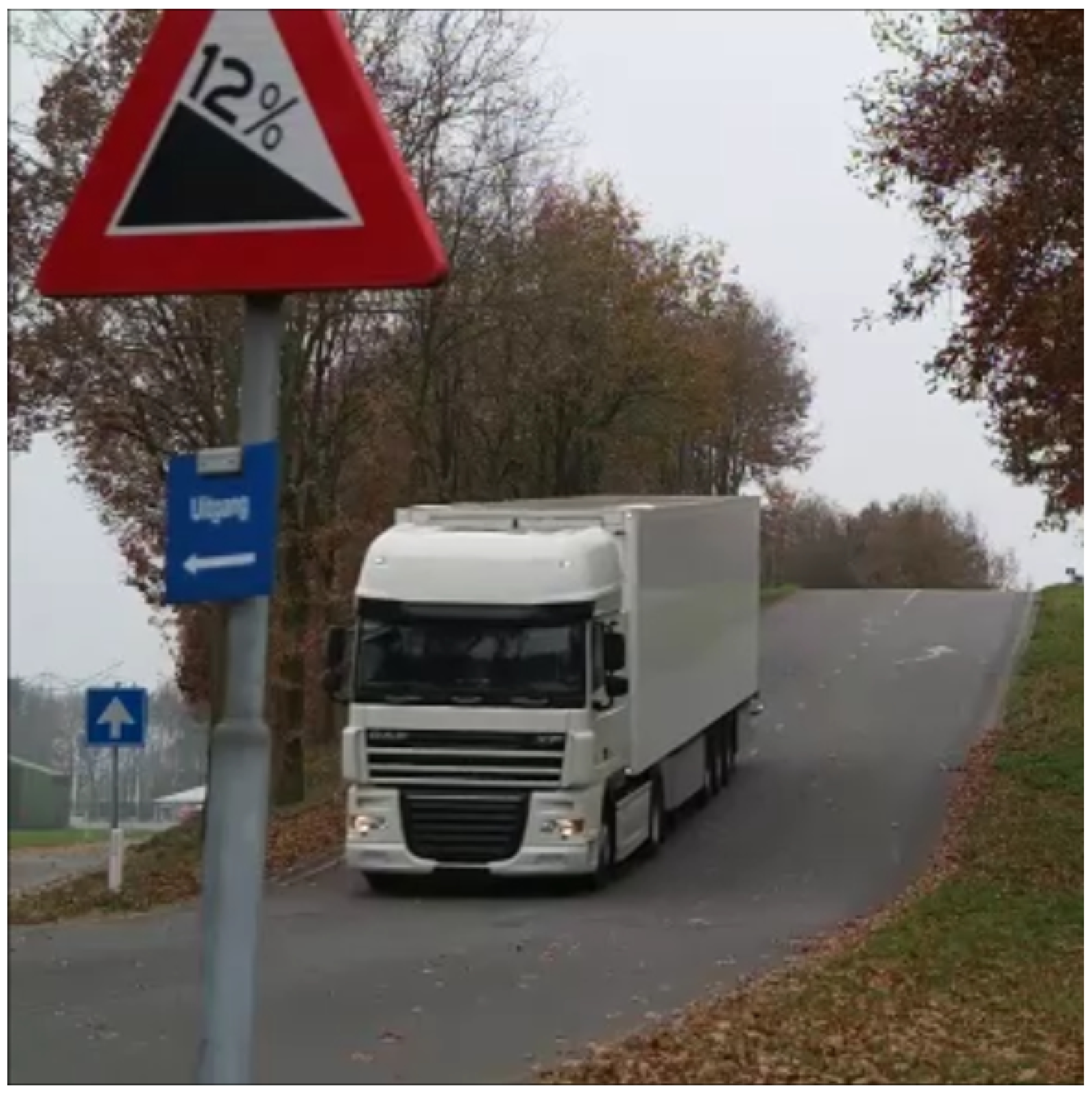
The hybrid electric vehicle (HEV) is a tractor trailer combination, shown in Figure 1. The topology of the parallel HEV contains a 340 kW combustion engine (CE), a 90 kW motor/generator (MG) and a 4 MJ Li-ion battery (BT), see Figure 3. Dependent on the intended weight, three vehicle configurations are used in the tests:

Figure 1.
The prototype DAF XF 105 hybrid electric vehicle is used for validation of the multi-level Energy Management System, on the proving grounds of DAF Trucks N.V.
- 10 ton, tractor only,
- 20 ton, tractor with light loaded, three-axle trailer,
- 40 ton, tractor with heavy loaded, three-axle trailer.
2.2. Test Track
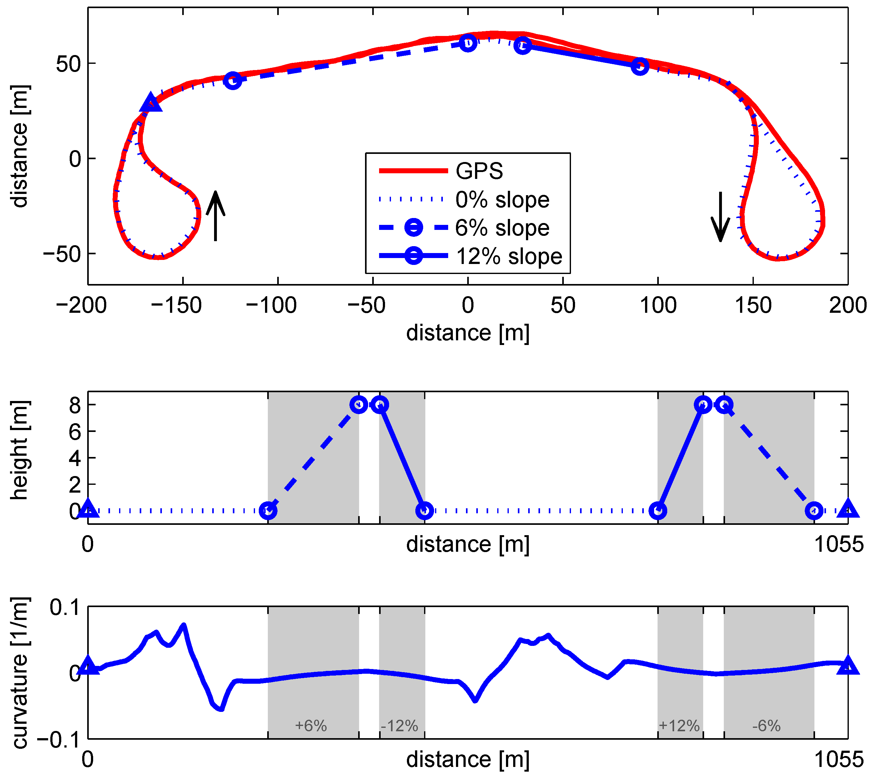
The EMS is tested on a route with elevation changes, thereby exciting the EMS functionality: different slopes cause a diversity in power levels for the drive train, necessitating mode and gear changes. To evaluate the robustness of the results, the same route is to be repeated, without disturbances such as traffic. Therefore, a route is selected on the DAF proofing grounds, containing elevation changes as shown in Figure 2. The plot contains the overview of the route, a repeatable cycle of 1055 m. In the center of the track, an 8 m high hill is positioned, containing a 6% slope and a 12% slope. At either side of the hill, a U-turn changes the driving direction. For a tractor trailer combination, the road curvature in the U-turns is significant. For safe cornering, the vehicle speed must remain below 25 km/h. For EMS validation purposes, the following characteristics should be noted:
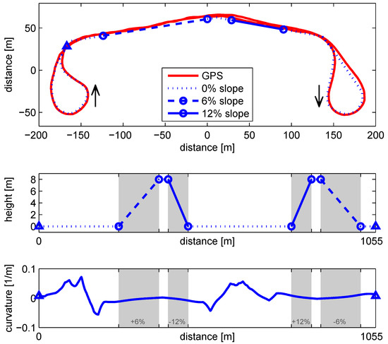
Figure 2.
Test track, with the location of the slopes. Measured GPS positions (red) are overlaid on the map data (blue). Distance measurement is started at the blue triangle, taking the U-turn, and followed by the +6% slope. After 1055 m the test cycle repeats. The curvature in both U-turns is significant, thereby limiting the maximum speed.
- The variation in slope from −12% to 12% causes a large range of road loads, covering all EMS functionality.
- The slope changes faster than on public roads, causing a high dynamic road load for the EMS.
- At low speed more gear selections are viable (typically 5), opposed to high speed driving, where gear selection is often saturated in the highest gear. Low speed driving is thus a more extreme test scenario for the EMS.
- The low speed compared to typical highway applications causes non-typical fuel economy numbers. However, the same fuel-saving mechanisms are present, which are validated in this research. Representative fuel economy numbers are calculated in a high-fidelity simulation environment ([14], Section 7.3), using these validated models.
Although the conditions on the test track deviate from typical highway application, they are more strenuous for the EMS, especially concerning the faster dynamics, involving power split, hybrid mode, and gear selection. These fast dynamics are typically approximated in high-fidelity fuel simulation environments, resulting in a mismatch between simulation and real-life control, whereas the effect of the slower dynamics (e.g., battery and vehicle longitudinal dynamics) are well captured. With the chosen route, specifically the faster dynamics are excited, thus creating a good complement to the high-fidelity simulation results, as presented in [14], Section 7.3.
2.3. Energy Management System Implementation
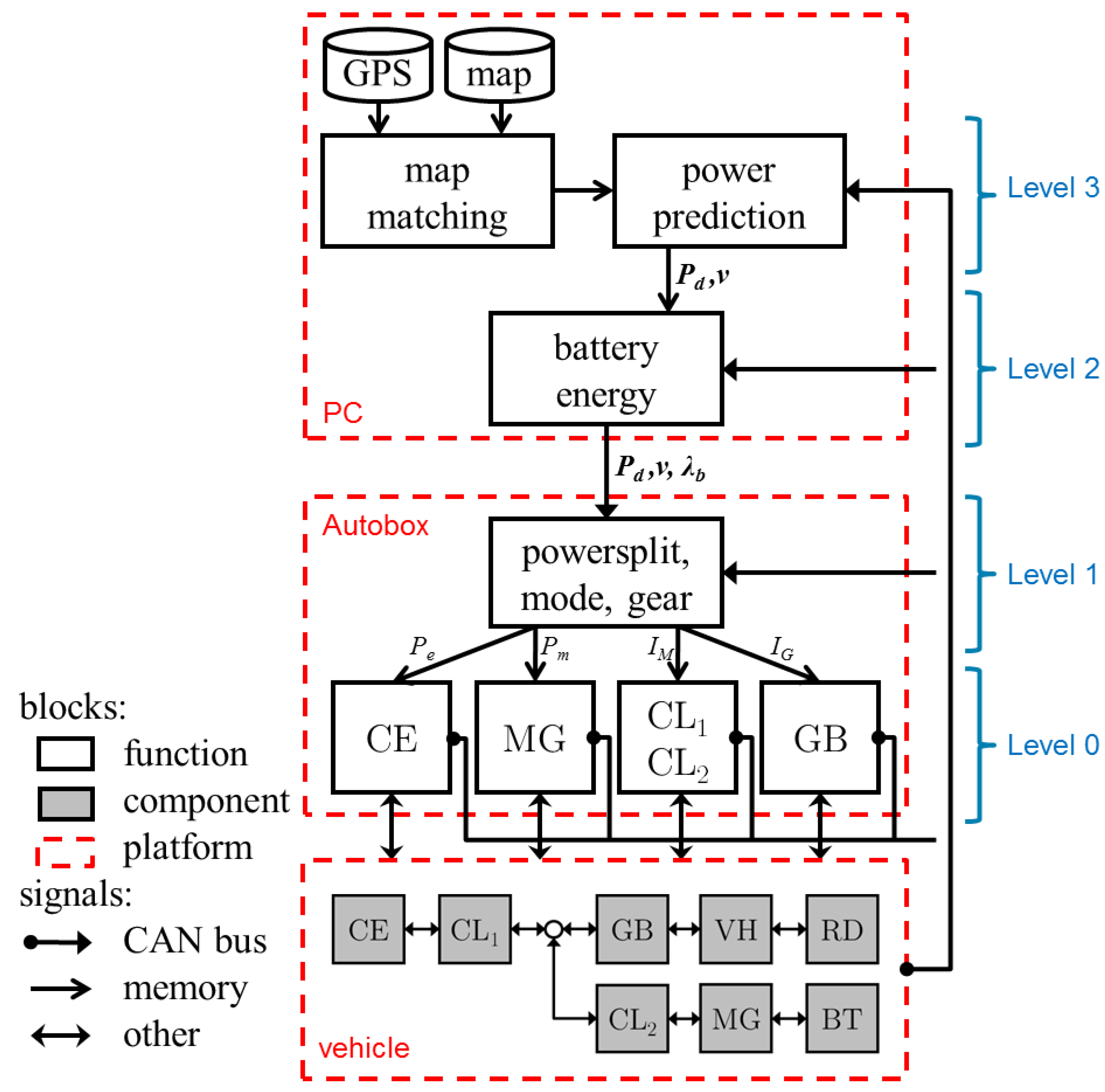
The multi-level EMS from [14] is implemented on the HEV. The algorithms on each level are mapped to two control platforms as depicted in Figure 3. Level 0 and 1 are running as compiled code on a dSpace Autobox to provide fast and predictable algorithm execution under all circumstances (i.e., ‘hard real time’). Level 2 and 3 are running on a PC as MATLAB code, facilitating the development of optimization algorithms, which have typically less strict real-time characteristics (i.e., ‘soft real time’). The minor coupling between the two control platforms improves robustness and facilitates parallel function development.

Figure 3.
Control function architecture with function mapping of the implemented strategy on the control platforms (Autobox and PC) of the vehicle. The parallel hybrid vehicle connects the 340 kW compression ignition engine (CE) and the 90 kW motor/generator (MG), each with a clutch (CL1 and CL2), to a 12-gear stepped transmission (GB), that drives the rear wheels of the vehicle (VH). The Li-ion battery (BT) has an effective capacity of 4 MJ. Component control on Level 0 provides an interface for the higher-level functions to the hardware. Level 1 functionality determines the setpoints for the components, based on processed preview information from Level 2 and Level 3. Communication between platforms is mainly over CAN, which is the standard communication bus in heavy-duty vehicles.
Of all Level 0 components, complete status information is available on the CAN bus. In addition, the relevant signals of the EMS are made available on that same bus and the complete CAN bus is recorded with a data logger. As such, the presented signals are reported values from the components itself, of which some are calculated, e.g., battery energy, engine power, and motor power. The reported values have shown to be consistent among the different subsystems and are separately validated on a roller bench. In the following sections, the implementation details are given for each level.
Level 0: Component Control
The Level 0 functions provides an interface to the physical components on the vehicle, i.e., the internal combustion engine (CE), motor generator (MG), clutches (CL1, CL2) and gearbox (GB). Level 0 translates the setpoints from Level 1, i.e., CE power , MG power , hybrid mode and gear , into proper and safe control of the components, and reports the relevant component capabilities to the higher-level algorithms over CAN. e.g., when a mode change is commanded to the clutches (CL1 and CL2) in Level 1, Level 0 first determines if it is safe (regarding e.g., speed, load or temperature) to perform the transitions, and if allowed, controls the transition of stopping, starting, and synchronization, continuously reporting the status of the clutches.
Level 1: Power Split, Mode, Gear Control
Level 1 calculates the power split () and the desired hybrid mode and gear , based on information from the components (Level 0) and route information from the levels above: the predicted power demand , velocity and cost equivalence . The switching costs of mode () and gear (), are fixed to 10 kJ and 20 kJ, respectively. The optimization is performed over a receding horizon, where every sample time, over a horizon of s, the decision variables are optimized. The samples of the prediction vectors and velocity , corresponding to the current time and position, are replaced by the current (measured) values and v. The update frequency of the algorithm is 100 Hz, to ascertain sufficient responsiveness of the controller to the power demand, posed by the driver or the speed control system. As Level 1 and Level 0 functionalities are both mapped on the Autobox, the signals are directly transferred through memory. Information from the higher levels is communicated over the CAN bus.
Level 2: Battery Energy Control
Level 2 calculates the costate , that optimizes the battery energy () trajectory within its bounds. The power split, and the desired hybrid mode are optimized, given the predicted power demand and assuming a constant engine speed . The sample time of the receding horizon algorithm is 1 Hz, with a horizon of 1000 s. The PC sends over CAN to Level 1 on the Autobox, together with and from Level 3.
Level 3: Power Prediction
Level 3 predicts the driveline power, based on geographic map data of the route ahead. It determines the current position of the truck using a GPS sensor, projected on a digital map (so-called ‘map matching’), and returns the slope and speed limits for the predetermined route. With this distance-based information, the speed profile is determined and the power demand is predicted. In our tests, the speed is controlled by a prototype speed controller, which has a set speed () of 24 km/h for cruising (positive traction), and a so-called downhill speed controller (DSC) for negative traction (braking), which has a set speed of 27 km/h, but is not included in the prediction. The Level 3 algorithm uses a horizon of 10 km, therefore repeating the test cycle of 1055 m 10 times. As the vehicle travels along the route, the calculation of and is updated with 1 Hz.
Computational Load
Level 0 functionality runs at 100 Hz on the dSpace Autobox, with a turnaround time of 0.3 ms. Level 1 functionality adds another 0.4 ms, mainly caused by the computationally demanding DP algorithm. That is a significant increase in load, but still comfortably below 7% at a 10 ms sample time. Level 2 and Level 3 algorithms run as MATLAB m-code on a laptop with Intel T9300 processor, demanding together less than 10% processor load.
3. Validation Level 3: Power Prediction
Level 3 predicts the driveline power, based on geographic map data of the route ahead. Using the vehicle position measured by the GPS sensor, the position on the map is determined (i.e., ‘mapmatching’) and for the known route ahead, slope information is retrieved from the map. With the algorithm as described in [14], Section 6, the power demand is predicted. The validation of the power prediction is performed by testing the repeatability on a repeated test cycle and varying vehicle parameters, i.e., the vehicle mass. Level 2 (Section 4) and Level 1 (Section 5.2, variant EMS7) algorithms close the loop.
3.1. Repeatability
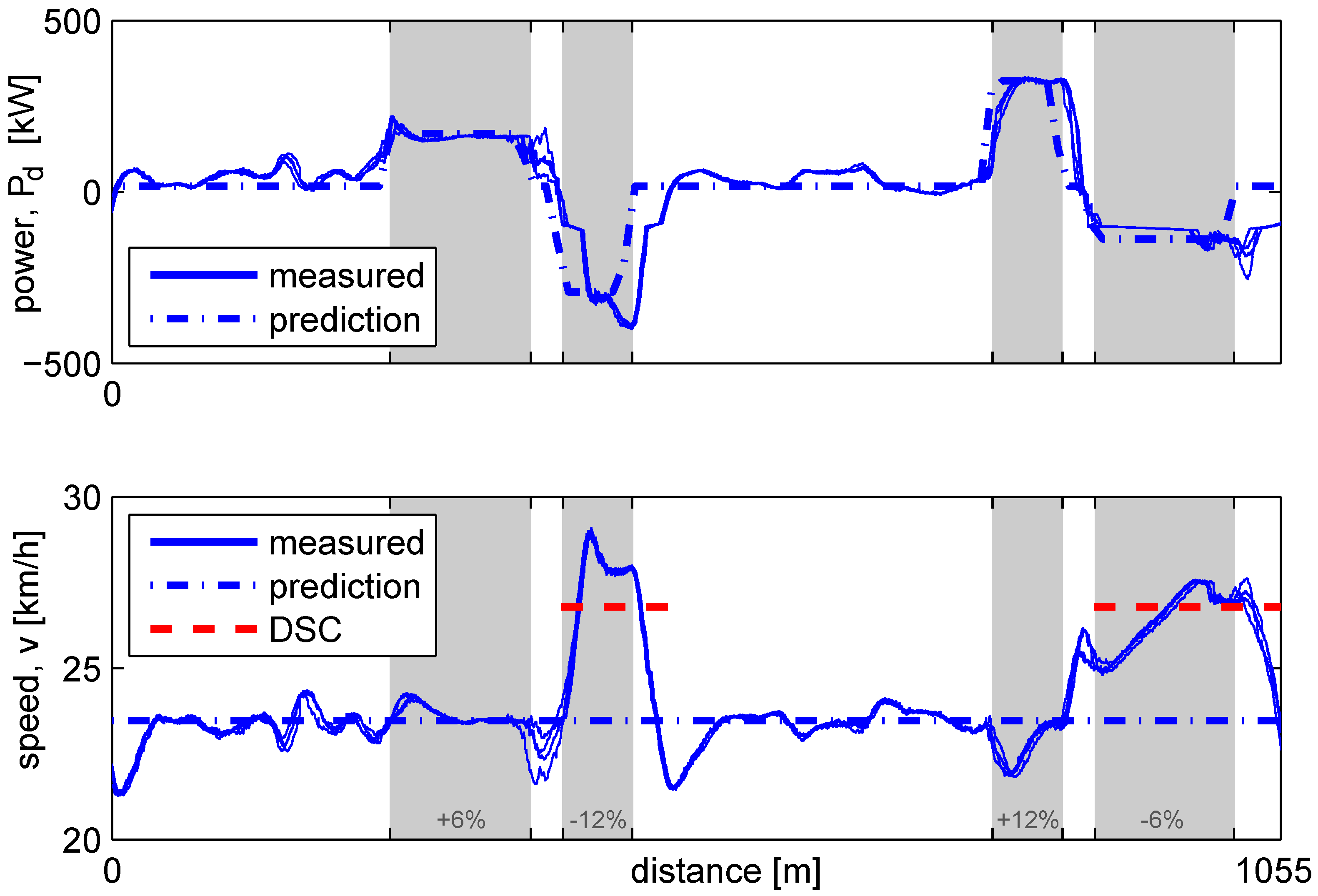
Repeatability of the power prediction is validated by running the 40 ton tractor trailer combination four times over the test track. The predicted power is compared with the instantaneous power as reported by the CE and MG, see Figure 4. The velocity is controlled by a prototype cruise control function with a set speed of 24 km/h for positive traction, while braking is controlled by DSC with a set speed of 27 km/h.
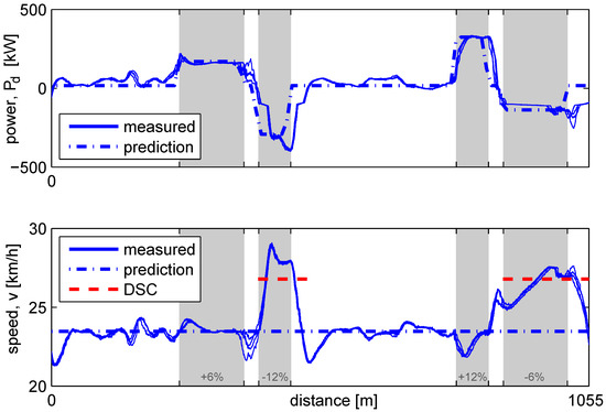
Figure 4.
Power demand and speed for repeating the test track four times, with the 40 ton vehicle. All four test runs have an exact overlay, with the only noticeable differences on the top of the hill. Unmodeled dynamics in the speed controllers, i.e., cruise control (blue dash-dotted setpoint) and DSC (red dashed setpoint), and unmodeled disturbances (i.e., cornering) cause deviations from the prediction (dash-dotted line).
The measured power demand (solid blue line in the top plot) and the measured velocity (solid line bottom plot) coincide closely for all four runs. Only minor differences can be observed between the measurements of the consecutive runs, with the largest difference at the top of the hill, where the 6% slope changes within 40 m to the 12% slope. There are, however, noticeable differences between the predicted and the measured power demand and speed:
- The predicted speed of 24 km/h is not maintained in the downhill (−12%, −6%) sections, where speed increases towards 29 km/h. This is caused by the design of the speed control system on the truck: cruise control is not allowed to apply braking. The DSC function is allowed to control the braking system but has a higher speed setpoint (27 km/h, indicated by the red dashed line). Due to the change in speed setpoint, some potential energy is temporarily converted to kinetic energy instead of brake energy, which is best illustrated on the −12% slope: during acceleration the measured braking power is smaller than predicted, while during the deceleration to the cruise setpoint the increased kinetic energy is converted to brake energy again, shown by the larger measured, than predicted, braking power.
- The measured power demand in the flat segments (0%) is often higher than predicted, but highly reproducible. The increased demands coincide with the sharp turns in the track as shown in Figure 2. The lateral acceleration caused by the sharp turns, increase the longitudinal friction forces due to tire slip and increased steering angles [15], especially with the 3-axis trailer with non-steering axles. This effect is not modeled in the previewer, as it depends on parameters not known to the EMS, such as tire temperature, tire compound, and vehicle configuration.
- The measured speed shows overshoot and undershoot near the slope changes. The slope changes on the track are extreme compared to public roads: within 5 m the slope changes from 0% to 6% (or 12%) and vice versa, resulting in large transients in the road load. At the same time, mode changes are commanded, see Section 5, resulting in a brief period without traction due to the open driveline. The tuning of the speed controllers is less suited for these extreme conditions, resulting in overshoot and undershoot behavior.
The repeatability of the measurement is high: from run to run the average standard deviation is less than 8 kW and 0.12 km/h. Due to unmodeled behavior of the speed controllers and cornering, the mean absolute error (MAE) between measurement and prediction, defined as:
with n the number of samples for the test run, is larger: 50 kW and 1.2 km/h. The largest errors, 400 kW and 5 km/h, occur around the slope changes.
3.2. Parameter Variation
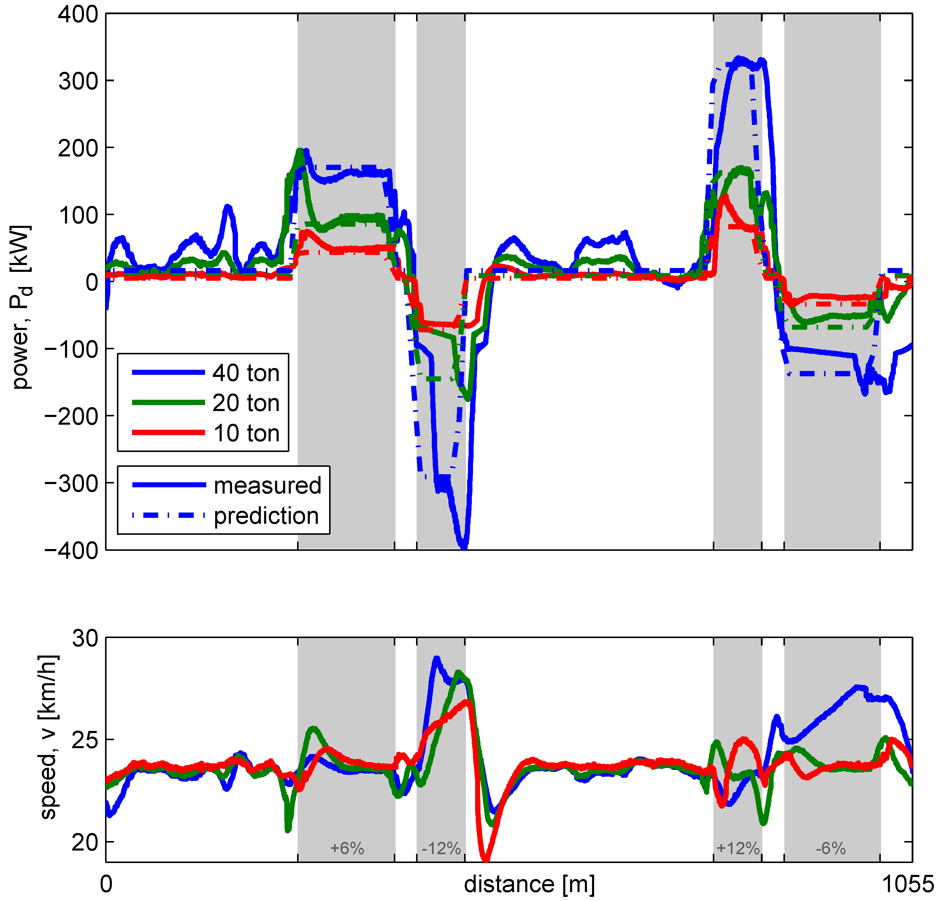
The accuracy of the prediction is influenced by the vehicle parameters, where the vehicle mass has a very large influence on the predicted road load. Validation of this parameter variation is performed by driving with the vehicle configurations from Section 2.1, resulting in three vehicle masses: 10, 20 and 40 ton. The mass parameter in the prediction, is updated using the onboard mass estimation of the vehicle. In Figure 5 the predicted and measured power demand are shown for each configuration.
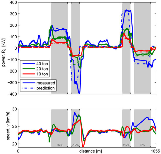
Figure 5.
Measured power demand and speed for three vehicle masses, compared to the prediction.
Comparable differences between prediction and measurement as in the previous section can be observed, but with a different effect for each mass:
- On the downhill sections, speed cannot be maintained for the 40 ton combination. On the −6% slope, MG-only recuperation is sufficient to maintain speed for the 10 ton and 20 ton configuration. On the −12% all configurations accelerate; however, the 10 ton tractor can do without DSC activation, resulting in a better match with prediction at the end of the −12% slope.
- In the sharp turns, located in the flat segments, the measured power demand is higher than the prediction, for the configurations with a trailer. As the three-axle trailer has no steering, large friction forces cause a high road load, most noticeable for the 40 ton configuration. The solo trailer has no significant prediction error in the turns.
- Where the slope changes and, at the same time, modes are changing, speed controller overshoot and undershoot is most noticeable for the heavy configurations.
During steady state conditions, where the slope is constant, the curvature is zero and the speed control is at its setpoint, the prediction is close to the measurement. On this compact test cycle, steady state conditions are only approximated on the second half of the +6% slope, where it shows correct scheduling of the mass parameter.
In Table 1 the prediction error for the three vehicle configurations is given. Although the predicted power demand shows large differences with the measurement, the influence of the slopes is clearly visible, which form the basis of the decisions of the EMS. The Level 2 and Level 1 controllers perform the calculations with this predicted power demand. Taking into account cornering effects, open driveline events and dynamics of the speed control could improve the prediction.

Table 1.
Prediction on the test cycle shows errors in both power demand as velocity. The mean absolute error (MAE) is given for three vehicle masses.
4. Validation Level 2: Battery Energy Control
The Level 2 algorithm is responsible for calculating the cost equivalence for fuel optimal battery energy () usage, see [14], Section 5. The algorithm will realize charge-sustaining behavior (), while the battery energy is optimally used. In this section, the Level 2 charge-sustaining functionality is validated. Level 3 (Section 3) and Level 1 (variant EMS7, Section 5.2) algorithms close the loop. The conditions in the test scenario result in smooth controllability of the charge sustenance and is analyzed next.
Charge Sustenance
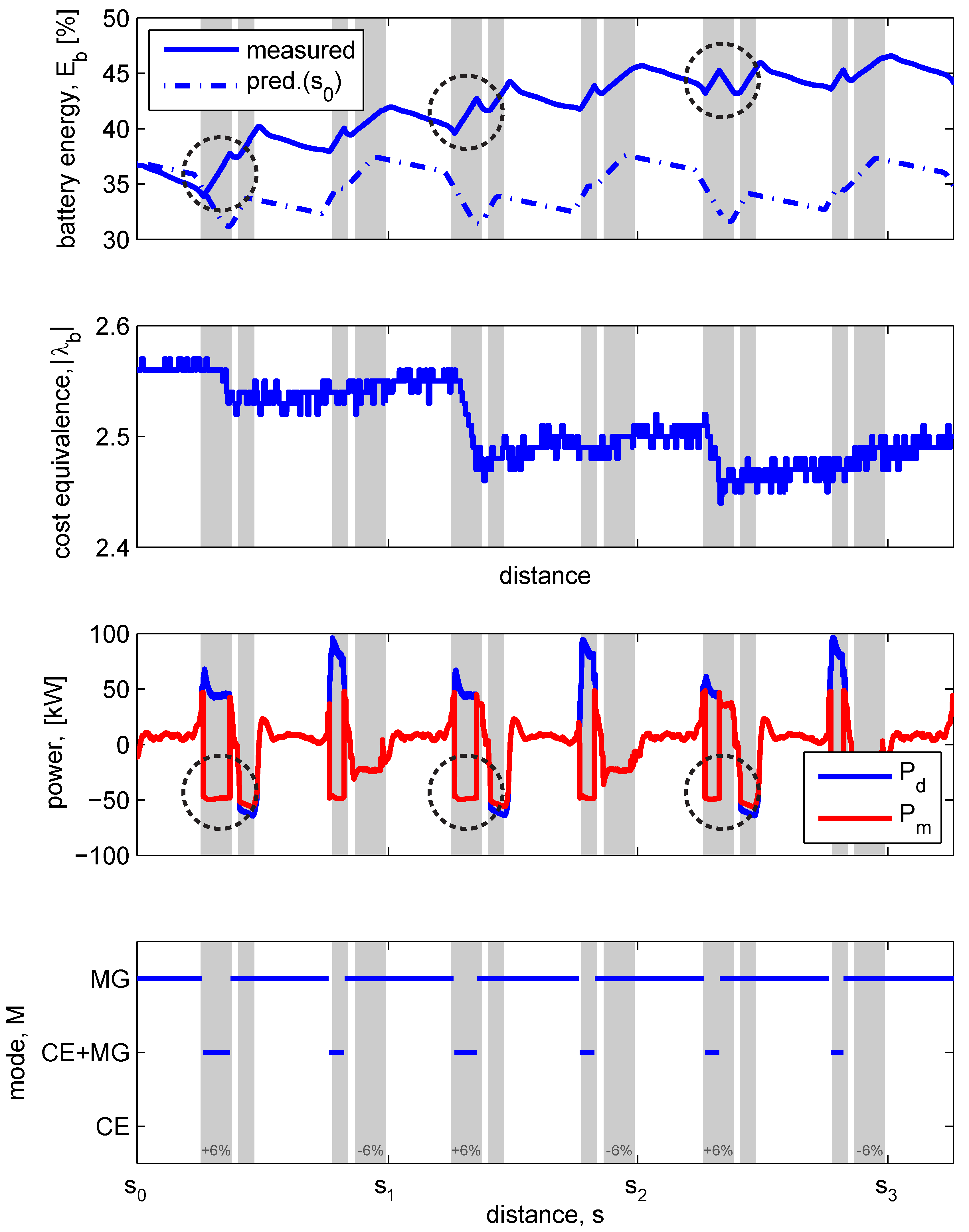
Charge-sustaining behavior in itself is not an objective, but it is a property of the fuel optimal solution on a cycle, when that same cycle is infinitely repeated. In this section, we use charge sustenance to show the feedback control of Level 2: each sample an optimization of the cost equivalence is made over the horizon of 10 km, starting with the latest (battery) state, to realize charge sustenance. The test is started with an arbitrary battery state and the 1055 m test cycle is repeated three times, with the 10 ton configuration, see Figure 6, to show the control of charge sustenance.
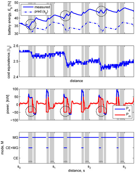
Figure 6.
Adaptation of the cost equivalence, to obtain charge sustenance after three cycles. Lowering the cost equivalence results in a shorter period of charging (where the power of the MG () is negative and thus is rising) on the +6% slope, indicated with the dashed circles. Besides the charging on the +12% slope, MG-only is selected for the rest of the cycle.
Starting at , the initial prediction of is plotted. For all three cycles, which are defined from to , from to and from to , the prediction expects charge-sustaining behavior, i.e., the same at , , and , for . While the vehicle progresses along the track, the error between predicted and measured increases and consecutive predictions (not shown) adjust to correct for the increased error, using algorithm I3 from [14], Section 5.3. After three cycles, Level 2 is close to charge-sustaining with = 2.46, with only 0.7% difference in remaining, see Table 2. It is expected that the fourth cycle will be charge-sustaining.
Table 2.
Charge sustenance of on three consecutive cycles.
The prediction error is caused by differences between the control model and the vehicle behavior:
- Level 2 power-split control uses a simpler abstraction of the vehicle (i.e., a fixed average engine speed and no cost on switching, [14], Section 4.2) than Level 1 power-split control (using the actual engine speed and penalized switching, [14], Section 4.3), where the latter implements its control to the components, while Level 2 only has as output.
- The real power demand is occasionally higher than the predicted power demand, as shown in Section 3. Level 1 is then forced to select a mode with higher power capabilities, than the predicted mode (MG-only) can deliver.
The corrective action of the feedback controller is acting mainly in one part of the cycle: the +6% slope. By lowering , the threshold for charging rises (see in [14], Figure 9), resulting in a shorter period of charging on the +6% slope, and to a lesser extent on the +12% slope. Because Level 2 calculates the corrective action over the whole horizon, it is able determine, where the corrective action improves the charge sustenance, with the least fuel penalty. On the rest of the cycle, the modes are identical from cycle to cycle. This contrasts with direct feedback control on the predicted trajectory, as is done in [3,16], where corrections take place whenever the error is large, and not per se where the cost is lowest.
5. Validation Level 1: Power-Split, Mode, Gear Control
Level 1 decides on the power split () and the desired clutch mode and gear , based on information from the components (Level 0) and route information from the levels above: the predicted power demand , velocity (Level 3) and cost equivalence (Level 2). On this level, the switching behavior of mode and gear determines the drivability and, combined with the power split, they determine the fuel economy of the EMS. On the test track three scenarios are considered:
- Base7: hybrid mode, with the power split and clutch mode controlled by a baseline, non-previewing, EMS. The gear is fixed in 7th.
- EMS7: hybrid mode, with the power split and clutch mode controlled by the Level 1 algorithm. The gear is fixed in 7th.
- EMSG: hybrid mode, with the power split, clutch mode and gear controlled by the Level 1 algorithm.
The validation in this section is performed with the 20 ton combination. For the scenarios Base7, EMS7 and EMSG, the decisions are analyzed in respectively Section 5.1, Section 5.2 and Section 5.3, with the energy efficiency compared in Section 5.4.
5.1. Power Split and Mode Selection (Base7)
The baseline, prototype, EMS uses heuristics without preview information to determine the power split, mode, and gear selection. It is tuned for fuel efficiency and is a baseline EMS for this prototype vehicle. When both mode and gear decisions are implemented, too much open driveline events occur, due to the extreme slope changes on the test track, resulting in aborted test runs. Therefore, the selected gear is fixed, such that the complete cycle can be driven without aborts, and the power split and mode decisions can be analyzed. A test run with charge-sustaining behavior () is selected, for the analysis in this section.
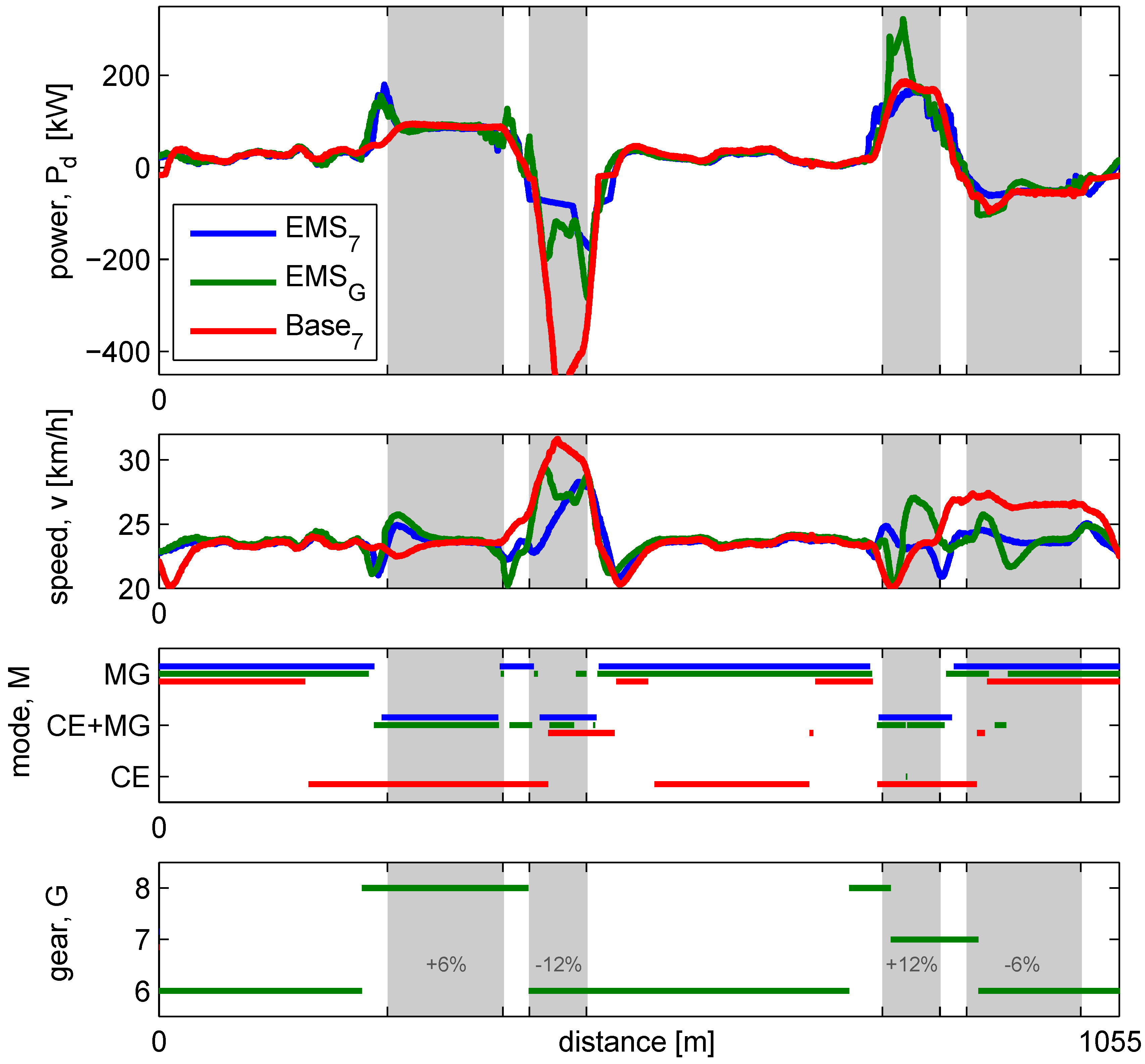
Figure 7 shows, from top to bottom, the measured power demand and velocity, and the mode and gear decisions. For Base7, large speed overshoots and undershoots occur near the 12% slope. Because this EMS must rely on feedback, it is typically too late in implementing a mode switch, resulting in large speed deviations due to the open driveline event on the slope. On the −12% slope the correct mode is eventually selected, where the braking power of CE+MG is needed to control the speed.
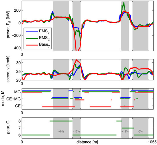
Figure 7.
Mode and gear decisions compared of EMS7, EMSG and Base7. The large speed deviations between the test cases, prevent a direct fuel comparison; however, based on the control decisions, fuel-efficient operation is identified.
On the flat segments the power demand is low, which could be driven with MG-only. Due to the selected modes, the CE is running for 60% of the time, often at low, inefficient, loads. Furthermore, the EMS is not consistent in the choice of mode: each type of segment is expected to be driven in one typical mode; however, with this prototype controller many unnecessary mode changes occur.
5.2. Power Split and Mode Selection (EMS7)
EMS7 implements Level 1 functionality, with gear decisions disabled, to compare with Base7.
Figure 7 shows the decisions of EMS7 with the resulting power demand and speed of the vehicle. With this controller, the speed deviations are smaller than with Base7, caused by the reduced amount of mode switches, and thus open driveline events. Due to the design of the speed control system in combination with braking, the speed deviation on the −12% is still present, as the setpoint changes from 24 km/h to 27 km/h.
The choice of modes is extremely different compared to Base7: more than 72% of the time the CE is stopped, driving the vehicle in MG-only. To generate enough energy for MG-only driving, the algorithm calculates that it is sufficient to charge the battery downhill and when the CE can operate efficiently: on the uphill slopes. On the −12%, MG-only is insufficient to maintain speed and the CE must support in braking. The measured mode selections are identical to the off-line simulated modes in [14], Section 7.2, thereby showing the intended fuel-efficient behavior of the Level 1 algorithm.
5.3. Power Split, Mode and Gear Selection: (EMSG)
EMSG implements Level 1 functionality, with the gear decisions enabled, having a penalty on shifting kJ. In Figure 7 the gear selection is ranging from 6th to 8th. The gear selection is mainly determined by the operation of the CE, as the friction of the CE is large and low rotational speeds minimize the friction. A large amount of mode changes takes place, some within a very short period of time, caused by:
- The amount of open driveline events is larger than with mode changing only, resulting in larger speed deviations. On the vehicle it was not possible to switch gears and modes simultaneously. Both events result in an open driveline condition of approximately 1 s, in total 2 s without traction, leading to large speed deviations from the speed setpoint. As a consequence, the integral action of the speed controller results in overshoot in the power demand, which in turn forces mode changes that are not foreseen by the previewer.
- Optimal gear shifting causes operation closer to the boundaries of the component power capabilities, as lower rotational speeds result in lower losses, however, also result in a lower maximum power. As the operating points are closer to the boundaries, deviations in the power demand will force a mode change or shift when the boundary is exceeded. This happens near the −12% slope for MG-only (mode change), but also for the CE+MG in the +12% segment, forcing a downshift from 8 to 7.
While the general idea of the mode and gear decisions make sense, the amount of switchings is too high. The following measures would improve the performance, but are currently not implemented:
- Change the gear shift penalty , dependent on the hybrid mode and road load, instead of one constant penalty for all conditions.
- Include the open driveline events in the control model, in order to correctly predict the speed, including overshoot and undershoot.
- Implement simultaneous mode and gear switching on Level 0, to reduce the open driveline time.
- Improve the speed controllers, to prevent short spikes in power demands.
5.4. Energy Consumption
The decisions on Level 1 control the behavior of the vehicle, resulting in the energy consumption over the test cycle. All EMS’s aim for charge-sustaining operation; however, in the measurements, minor differences exist between the battery energy at the start and the end of the cycle. That difference is compensated by using the equivalent fuel consumption, which is the fuel consumption (here: as reported by the CE), corrected with the difference in battery energy multiplied by the costate. In Table 3 the equivalent fuel consumption J is shown for each EMS, driving one cycle on the test track.
Table 3.
Comparison of the energy consumption of the EMS’s, for one cycle on the test track.
The energy reduction of the EMS’s varies between 24% and 36%. The measured energy reduction of EMSG (34%) is smaller than the simulated energy reduction (53%) in [14]. The difference is caused by:
- a higher power demand on the cycle than simulated, mainly caused by the un-modeled cornering effect. This results in much higher average power demands on the flat segment (25 kW instead of the predicted 9 kW), which results in a smaller energy benefit of selecting the optimal mode (MG-only instead of ICE-only).
- missing some brake energy on the −6% incline for the fixed gear EMS’s. A downshift is needed to use the maximum recuperation power of the MG.
- too many switching events, reducing the potential of EMSG.
Even though the power demand is higher than predicted, the EMS7 selects the optimal modes, belonging to the higher power demand. This is the result of the Level 2 battery energy optimization, which adjusts the cost equivalence, causing the amount of battery charging to be balanced with the increased energy demand of electric driving on the flat segments. On the track the EMS7 is able to reduce fuel consumption with 36% compared to the non-hybrid, which is a large improvement over the 24% of the baseline strategy.
6. Conclusions and Recommendations
In this work, the multi-level optimization-based EMS from [14] is validated with a heavy-duty hybrid vehicle on a test track. The real-time implementation of the previewing EMS is shown to be feasible on state-of-the-art hardware and results in improved behavior compared to the baseline strategy, both in drivability and fuel-saving principles. Un-modeled open driveline effects currently limit the practical applicability of the gear selection algorithm; however, possible solutions are given. Validation of the complete EMS is performed, and for each control level the following sub-conclusions are drawn:
6.1. Power Prediction
The map matching and power prediction on Level 3 are shown to work well for the route: the reproducibility of the road load is large and in steady state situations, where velocity, curvature, and slope are constant, the prediction is close to the measurement. Large errors, however, occur during unpredicted transients. >From the measurements it is clear that the power demand prediction can be improved by incorporating the behavior of the speed controllers. The prediction assumes constant speed where possible, whereas the real speed controller has switching (between cruise control and DSC) and overshoot behavior. Driving with different vehicle configurations causes changes in the power prediction, where mass variation is clearly accounted for, but cornering friction with a non-steering trailer is not included. For less dynamic cycles, such as highway driving, the current prediction is expected to be sufficient, as cornering and slope changes will be less aggressive.
In future work the velocity should be incorporated in the EMS, thereby improving the interaction between power and velocity control, noticeable on Level 1. Furthermore, with more information of the environment of the truck becoming available, e.g., with radar, cameras, vehicle-to-vehicle, and vehicle-to-infrastructure communication, the quality of the power and velocity prediction will be improved.
6.2. Battery Energy Control
Level 2 battery energy control is validated on the test track by showing how the battery energy is controlled towards charge-sustaining behavior, which is a property of the optimal solution. The receding horizon control on the costate (or Lagrange multiplier), is shown to compensate for errors in the control model and the prediction, in a cost optimal way.
6.3. Power Split, Mode and Gear Selection
Three Level 1 EMSs are evaluated on the test track: Base7, EMS7 and EMSG. The EMSs are shown to operate on the test track, with large conceptual differences in the mode decisions. To drive the track, the gear setting had to be fixed for the baseline, non-previewing, strategy Base7. Under the fixed gear constraint, a comparison is made with the previewing strategy EMS7, which shows close-to-perfect mode selection: the amount of switch events is minimal, and optimal modes for fuel efficiency are selected, e.g., by correctly predicting and implementing, when the CE can be turned off. EMSG includes gear shifting, showing potentially better performance than EMS7; however, the amount of open driveline events increased, due to larger deviations from the predicted power and speed. A suggested solution to the problem is to model the speed and power demand during, and after, an open driveline event, and use a variable penalty on switching, dependent on hybrid mode and road load.
6.4. Discussion
The proposed EMS is shown to be robust against disturbances from the environment, such as higher-than-predicted power demands and deviations from the predicted vehicle velocity. The decisions of the EMS show the same behavior as the optimal solution, as presented in [14]. Improved performance is expected, when more information of the disturbances is available, and with little adjustment to the EMS, that information can be taken into account, e.g.,
- Including un-modeled friction effects. In the tests, cornering with a trailer showed large disturbances in the power prediction. In situations such as low speed maneuvering in sharp corners, modeling this effect will reduce the power prediction error and will improve the fuel-efficient decisions of the EMS. In long-haul applications, sharp cornering has no significant relevance in the energy consumption, and this effect can be neglected, without loss of fuel efficiency.
- Prediction of the velocity. The presented EMS uses a simple model of the environment, assuming that the vehicle can always drive its intended velocity. The environment however can force the vehicle to deviate from its intended velocity, e.g., by front runners, traffic lights, crossings, or heavy traffic ahead. Information that describes the environment better, can improve the estimation, e.g., from a radar system that tracks the front runner, or from online connected systems that inform the vehicle of heavy traffic ahead. That information can be used to improve the prediction on Level 3. The lower level algorithms automatically take the improved information into account, by the respective predicted velocity and power demand, with no further alterations in the algorithm needed. Future work is aimed at improving the Level 3 power and speed prediction, by including those additional information sources.
Author Contributions
V.v.R. developed the presented methodologies and conducted the experiments and validation. He performed writing and editing of the original draft. T.H. was responsible for supervision, internal reviewing and editing of the draft and concepts.
Funding
This research was funded by the Dutch Ministry of Economic Affairs, Agriculture and Innovation via the High Tech Automotive (HTAS) Program for the Hybrid Innovations for Trucks (HIT) project.
Acknowledgments
This research was supported by DAF Trucks N.V. and the Eindhoven University of Technology.
Conflicts of Interest
The authors declare no conflict of interest.
References
- Sciarretta, A. A control benchmark on the energy management of a plug-in hybrid electric vehicle. Control Eng. Pract. 2013, 29, 287–298. [Google Scholar] [CrossRef]
- Delprat, S.; Guerra, T.M.; Rimaux, J. Optimal control of a parallel powertrain: From global optimization to real time control strategy. In Proceedings of the IEEE Vehicular Technology Conference, Vancouver, BC, Canada, 24–28 September 2002. [Google Scholar]
- Ambühl, D.; Guzzella, L. Predictive Reference Signal Generator for Hybrid Electric Vehicles. IEEE Trans. Veh. Technol. 2009, 58, 4730–4740. [Google Scholar] [CrossRef]
- Hellström, E.; Åslund, J.; Nielsen, L. Management of Kinetic and Electric Energy in Heavy Trucks. SAE Int. J. Engines 2010, 3. [Google Scholar] [CrossRef]
- van Reeven, V.; Huisman, R.; Pesgens, M.; Koffrie, R. Energy Management Control Concepts with Preview for Hybrid Commercial Vehicles. In Proceedings of the 6th International Conference on Continuously Variable and Hybrid Transmissions, Maastricht, The Netherlands, 17–19 November 2010. [Google Scholar]
- Merz, F.; Sciarretta, A.; Dabadie, J.C.; Serrao, L. On the optimal thermal management of hybrid-electric vehicles with heat recovery sytems. Oil Gas Sci. Technol. 2012, 67, 601–612. [Google Scholar] [CrossRef]
- Serrao, L. A Comparative Analysis of Energy Management Strategies for Hybrid Electric Vehicles. Ph.D. Thesis, The Ohio State University, Columbus, OH, USA, 2009. [Google Scholar]
- Nüesch, T.; Elbert, P.; Flankl, M.; Onder, C.; Guzzella, L. Convex optimization for the energy management of hybrid electric vehicles considering engine start and gearshift costs. Energies 2014, 7, 834–856. [Google Scholar] [CrossRef]
- Ngo, V.; Hofman, T.; Steinbuch, M.; Serrarens, A. An optimal control-based algorithm for Hybrid Electric Vehicle using preview route information. In Proceedings of the American Control Conference, Baltimore, MD, USA, 30 June–2 July 2010; pp. 5818–5823. [Google Scholar]
- Kermani, S.; Trigui, R.; Delprat, S.; Jeanneret, B.; Guerra, T.M. PHIL implementation of energy management optimization for a parallel HEV on a predefined route. IEEE Trans. Veh. Technol. 2011, 60, 782–792. [Google Scholar] [CrossRef]
- Elbert, P. Noncausal and Causal Optimization Strategies for Hybrid Electric Vehicles. Ph.D. Thesis, ETH Zurich, Zurich, Switzerland, 2013. [Google Scholar]
- Van Keulen, T.; van Mullem, D.; de Jager, B.; Kessels, J.; Steinbuch, M. Design, implementation, and experimental validation of optimal power split control for hybrid electric trucks. Control Eng. Pract. 2012, 20, 547–558. [Google Scholar] [CrossRef]
- Back, M. Pradiktive Antriebsregelung zUm Energieoptimalen Betrieb von Hybridfahrzeugen. Ph.D. Thesis, Universitat Fridericiana Karlsruhe, Karlsruhe, Germany, 2005. [Google Scholar]
- Van Reeven, V.; Hofman, T. Multi-level energy management for hybrid electric vehicles—Part I. Vehicles 2018, in press. [Google Scholar]
- Pacejka, H.B. Tire and Vehicle Dynamics; Elsevier: Amsterdam, The Netherlands, 2012. [Google Scholar]
- van Keulen, T.; de Jager, B.; Kessels, J.; Steinbuch, M. Energy Management in Hybrid Electric Vehicles: Benefit of Prediction. In Proceedings of the IFAC Advances in Automotive Control, Munich, Germany, 12–14 July 2010. [Google Scholar]
© 2019 by the authors. Licensee MDPI, Basel, Switzerland. This article is an open access article distributed under the terms and conditions of the Creative Commons Attribution (CC BY) license (http://creativecommons.org/licenses/by/4.0/).